Application of an Improved Convolutional Neural Network Algorithm in Text Classification
Jing Peng1,* and Shuquan Huo2
1School of Philosophy, Anhui University, Hefei, 230039, China
2School of Philosophy and Public Management, Henan University, Kaifeng, 475004, China
E-mail: pjgoodluck@126.com
*Corresponding Author
Received 03 February 2024; Accepted 14 March 2024
Abstract
This paper proposes a text classification model based on a combination of a convolutional neural network (CNN) and a support vector machine (SVM) using Amazon review polarity, TREC, and Kaggle as experimental data. By adding an attention mechanism to simplify the parameters and using the classifier based on SVM to replace the Softmax layer, the extraction effect of feature words is improved and the problem of weak generalization ability of the CNN model is solved. Simulation experiments show that the proposed algorithm performs better in precision rate, recall rate, F1 value, and training time compared with CNN, RNN, BERT and term frequency-inverse document frequency (TF-IDF).
Keywords: Text classification, convolutional neural network, support vector machine, attention mechanism.
1 Introduction
Being a key technology in natural language processing, text classification helps to solve the problem of accurate location for what the users need in information chaos [1–3]. Text classification is the process of categorizing a large amount of text into one or more categories based on the topic, content, or attributes of a document. The methods of text classification are mainly divided into two categories: rule-based methods and statistic-based methods. The former category often requires the support of knowledge and a rule base whose limitations of rule formulation and updating often confine it in certain specific fields due to its narrow application. In contrast, statistic-based methods generally rely on certain data or principles of statistics on the training set by establishing corresponding data models for learning about parameters through sample statistics and calculations to fulfill classifier training. Then, based on parameters learned from the training phase, categories of the samples could be predicted in the testing phase.
As the rule-based methods fall short of the need for a diversity of classification samples, a large number of statistic-based methods carry more weight. Schneider [4] applied naive Bayes to text classification in 1961, and pioneered machine learning algorithms in this regard. Later, models based on k-nearest neighbor (KNN) [5], maximum entropy (ME) [6], and CART [7] in the decision tree came in succession [8]. With the continuous development in research, Cortes et al. [9] proposed the support vector machine (SVM) algorithm and Joachims applied a version of the improved SVM model [10] to text classification, triggering a research boom since then for the great advantage of SVM in processing high-dimensional data sets. When the data vectors of different categories cannot be divided in the low dimensional space, SVM will map them to the high dimensional space through the kernel function and it searches for the optimal hyperplane for classification to improve the accuracy of text classification. Between the late 1990s and the early 21st century, the emergence of boosting algorithms further improved the precision and efficiency of text classification [11]. Joachims once conclusively made a comparative study between different machine learning algorithms including SVM, decision tree, KNN, integrated learning models, etc. and pointed out key problems in text classification investigation like nonlinearity, dataset skew, and annotation bottleneck among others. These models mentioned above are shallow analysis models. In practice, it has been proven that these models can only solve problems in simple situations or under multiple constraints. However, when faced with complex problems, the generalization ability of shallow analysis models and classifier ensemble methods will be limited and thus unable to meet specific requirements.
Compared with the shallow models, deep models are featured with abilities in self-learning and judgment. In the 21st century, especially after 2006, due to improved computing power, deep layer analysis models began to play a prominent role in the research of text classification [12]. A recurrent neural network (RNN) [13], a suitable model for sequencing text information data, is widely used. Arevian et al. [14] studied the application of the RNN model for real benchmark corpora. An RNN is capable of natural understanding of sequential text data. It has long-range memory ability to process better data of different lengths and shows strong integration coupled with high accuracy. Due to the gradient explosion in RNN, Hochreiter et al. [15] proposed a long short-term memory (LSTM) network, which adopted a gated storage structure with long-term and short-term memory mechanisms to solve the problem of long-range dependence in the RNN model. Yu et al. [16] combined Tokenizer word segmentation technology with the LSTM network to deal with multi-classification for Chinese texts. By comparing with traditional machine learning algorithms, Liang demonstrated that his model based on LSTM had a better classification effect. LSTM can effectively extract contextual feature information and has a good effect on long text processing. However, for short texts, especially those lacking contextual information, LSTM cannot capture local feature information. The BERT (bidirectional encoder representations from transformers) pre-training model based on bidirectional transformers has made breakthrough contributions to a large number of non-generative natural language processing tasks due to its excellent sentence-level feature extraction capability based on word vectors [17]. The BERT model effectively overcomes the disadvantage of the RNN and LSTM models’ inability to perform parallel computation, and due to the characteristics of its internal transformer self-attention module, it exhibits better “memory” ability in long-distance dependency problems [18]. However, since the BERT model is relatively complex and has a large parameter scale, it limits the number of tokens contained in the input sentence. To train long text that exceeds the input limit, only a portion of the content can be truncated as input.
The convolutional neural network (CNN), another neural network, was also widely used in text classification for its simple structure and ability to select features from different dimensions. In 2014, Kalchbrenner et al. [19] proposed DCNN, which adopts the dynamic k-max pool method to extract the relationships between words with different distances in a sentence. In the same year, Chen [20] proposed a TextCNN model which applied the CNN model to different data sets for topic classification and semantic analysis and got good results. Tao et al. [21] combined word2vec with CNN for short text classification, which greatly improved the precision rate compared with traditional machine learning algorithms. However, it is difficult for CNN to adjust specific features based on the training results when tuning the model and the generalization ability of the software layer is poor.
By combining the shallow and deep layer analysis models, this paper proposes an improved CNN model for English text classification. This model, a fusion of a CNN and a support vector machine (SVM) classifier, is added with an attention mechanism. With this algorithm, feature extraction of the data set is carried out through CNN while classification technology based on SVM is used to replace its normalized exponential function with insufficient generalization ability, which is supposed to improve efficiency and precision to a certain extent. By comparing with the CNN-SVM, TF-IDF (term frequency-inverse document frequency), RNN, and BERT algorithms, experiments have shown the feasibility and better performance of the proposed algorithm in certain aspects.
The rest of the paper is organized as follows. Section 2 is about text enhancement and preprocessing methods. Section 3 presents the text classification strategy based on the improved convolutional neural network. Section 4 presents the simulation experiment results for different performances. Finally, Section 5 concludes the paper and presents directions for future work.
2 Text Preprocessing Method
In order to increase the accuracy of text classification, the text is enhanced and preprocessed before classification.
2.1 Text Enhancement
This paper uses easy data augmentation (EDA) and back translation for text enhancement. After text enhancement, the number of samples in the dataset can be significantly increased, which is helpful for model parameters through training and alleviates the overfitting of few-shot learning models.
EDA includes the following four methods:
Synonym replacement: x words are randomly sampled from the input sample sequence and then to be replaced by their synonyms randomly selected from the corresponding synonym set. For example, “This book is so interesting that I read it all day.” becomes “This book is so entertaining that I read it all day.” after replacement.
Random insertion: Randomly sample a word from the input sample sequence, and select a position in the original input sample sequence to place its synonym.
Random exchange: Exchange two words randomly selected in the input sample sequence.
Random deletion: Based on experience and sample sequence length, set the proportion of words that can be deleted in the sample sequence. Randomly delete words from the input sample sequence at the set certain proportion. For example, “This book is so interesting that I read it all day.” becomes “book is so interesting I read it all day.” after random deletion.
These processes completed, the text is further enhanced by a back translation which translates sample data into an intermediate language and then from the intermediate language back to the original language. This is a common technique for text enhancement. After back translation, new sample data with the same meaning as the original ones in different expressions will be obtained. Compared with the original data, it is likely that the new sample data changed in sentence structure will have some words obtained such as the synonyms of the original words or the deleted ones from back translation.
2.2 Text Preprocessing
Text preprocessing comes after text enhancement. In this experiment, Stanford’s Global Vectors for Word Representation (GloVe) whose total size is 1.75 GB from the training of the super large dataset Common Crawl is used. The dimension of the pre-training word embedding is 300. After the word list is obtained, the text in the dataset is preprocessed as follows [22]:
1. Deactivated words such as “a” and “to” are deleted when training the GloVe word embedding, so these words are removed from the experimental training set data in this paper.
2. Some special symbols, including “$?!., #% () *+-/:;=”, etc. are removed.
3. For numbers, all those greater than 9 in the pre-training word embeddings are replaced by “#”. For example, “123” becomes “# # #” and “15.80” becomes “# #. # #”.
Finally, the cleaned dictionary (glossary) is used as the experimental input, which is a matrix of word embeddings composed of those selected from the dictionary.
3 Text Classification Strategy
In text classification, it is necessary to vectorize the originally high-dimensional and sparse words and map them to the low-dimensional and dense word vector space before model training. The CNN model uses the Softmax layer as the output layer. The essence of this layer is a full connection layer. Its function is to calculate the probabilities of different categories by a linear combination of feature words to realize a final classification. Since the Softmax layer does not work so well with those nonlinear and sparse data, this paper proposes a CNN-SVM model based on the combination of the CNN model and SVM classifier, which relies on the CNN model to select feature words and simplifies feature extraction while the SVM classifier is based on supervised learning to realize text classification. The network structure of this model is shown in Figure 1.
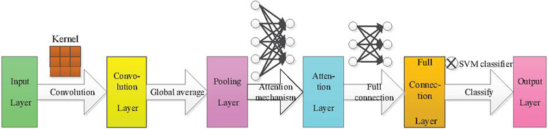
Figure 1 Network structure of the CNN-SVM model.
3.1 Convolutional Neural Network
(1) Text input
In this paper, the CNN network uses the continuous bag-of-words (CBOW) model based on the word2vec tool for word vectorization [23]. The word vector trained by the CBOW model constitutes the CNN-2 channel, which is used as the input layer of the CNN-SVM model. Using the CNN-2channel as the input layer of the model can not only ensure the meaning of the words themselves but also change according to different types of training sets to speed up the convergence of the model. In this study, it is assumed that background words correspond to a central word. These background word vectors are usually averaged to calculate the joint probability. and respectively represents the background word vector and center word vector corresponding to the words with index in the corpus. Assuming that the center word in the corpus and its background words as respectively. The conditional probability of generating the headword based on the given background words is:
| (1) |
when are denoted as , is denoted as , and Equation (1) can be simplified as
| (2) |
Suppose that in a text sequence with length , the background window size is and the words of an index are . Through the maximum likelihood estimation of the CBOW, the probability of generating the center word through background words is calculated as follows:
| (3) |
During CBOW model training, the calculation of maximum likelihood estimation is equivalent to solving the minimum loss function:
| (4) |
Equation (4) can be obtained by logarithmic operation:
| (5) |
The gradient of any background word related to conditional probability can be calculated by using a differential equation for Equation (5):
| (6) |
(2) Feature extraction
Feature extraction of text is achieved through convolutional and pooling layers. The convolution layer can limit the mapping relationship between the hidden units in the hidden layer and the input units in the input layer. Figure 2 shows how local perception is connected. The output neuron is only connected with the input neuron in the local area and is adopted in the local area in a fully connected manner; input neurons beyond the local range will have no connection. Local connections reduce losses compared to full connections, while also reducing the size of the parameter.
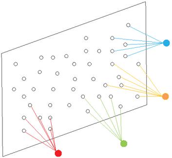
Figure 2 Local connection.
When the CNN model is applied to text classification, it is required that the dimension of the input layer word vector should be consistent with the width of the convolution kernel. Figure 3 illustrates a convolution operation on a two-dimensional matrix.
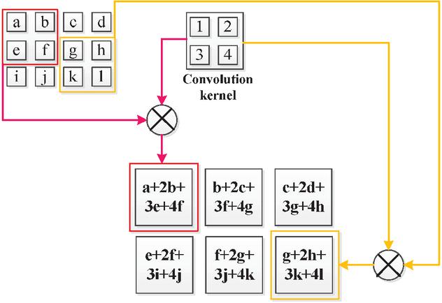
Figure 3 Convolution operation process.
The matrix, composed of , , and , represents the local perception, and the convolution kernel is composed of 1, 2, 3, and 4. By convoluting with the convolution kernel, the final result is . The input layer word vector is a matrix, the convolution kernel is a matrix, and the convolution step size is 1. According to the formula, the dimension of the feature graph obtained by the convolution operation is . When the input matrix is dimension and the convolution kernel is a matrix, the step size is , then the dimension of the feature graph obtained by the convolution operation is . In a simple neural network model, there is only one convolution kernel in one convolution layer. When the convolution network is applied to classification in this paper, due to the large vocabulary involved and the relevance of context Information in the text, multiple convolution kernels with different dimensions are often used for convolution operation to increase the precision of feature extraction. The convolution calculation formula is [24]
| (7) |
In Equation (7), the total number of convolution kernels is , represents that the operation starts from the first convolution kernel, represents the output result of a layer in the convolution layer, represents the weight value between layer and layer , and represents the bias term in the layer . is a nonlinear activation function in the convolutional neural network. Its function is to increase the convergence speed and solve the problems of gradient explosion and gradient disappearance to a certain extent. In this experimental environment, the activation function will adopt the Relu function. The purpose of using the activation function is to avoid the gradient disappearance of the model with the increasing number of layers.
Although the use of local connections can effectively reduce the scale of parameters, the number of parameters in the model is still very large, resulting in an unsatisfactory effect of model training. With weight sharing (as shown in Figure 4), only one convolution kernel is needed to fulfill the convolution operation of all word vectors and thus reduce the number of parameters to the greatest extent to accelerate the speed of model training.
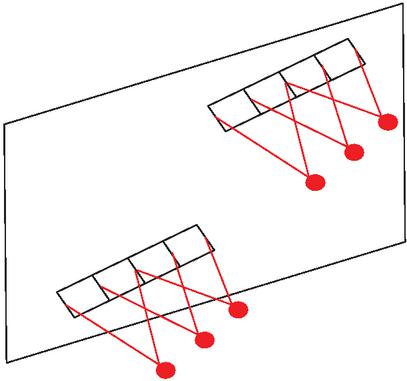
Figure 4 Weight sharing.
With local perception and weight sharing in the CNN model, a reasonable adjustment for the number of convolution layers and the size of the convolution kernel, which are mainly designed for different application scenarios, can be made in order to realize an optimal classification effect. Meanwhile, with the increase of convolution layers, its learning ability increases as well and so does the number of the feature words extracted.
The main work of the pooling layer is to reduce the dimensions of the convoluted data for better extraction of features. The output of this layer is adjusted by using the pooling function and the text feature vectors with lower dimension are extracted from the ones with higher dimension to replace the output of the network in this position. Common pooling methods include maximum pooling and average pooling which means extracting the average and maximum values of local feature vectors. The pooling layer can effectively reduce the size of the feature mapping, reduce the dimensions, increase the training speed of the model and prevent overfitting. Global pooling uses a sliding window of the same size as the feature graph, which ultimately pools the feature graph into one-dimensional data. As global pooling can greatly reduce the number of bits of parameters, it is thus adopted in the CNN-SVM model, as shown in Figure 5.
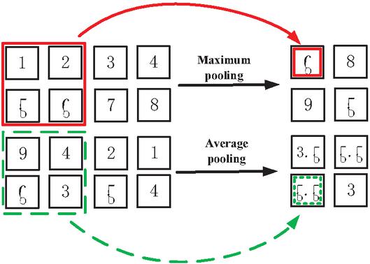
Figure 5 Maximum pooling and average pooling.
In Figure 5, a sliding window with a step length of 2 is adopted to carry out maximum pooling and average pooling respectively. The sliding window becomes one element after pooling, and the original feature graph becomes a feature graph after pooling, which greatly reduces the size of the feature graph.
(3) Attention mechanism
In the CNN-SVM model, the convolution layer and pooling layer fulfill the preliminary extraction and dimensionality reduction of feature words by training the word vector of the input layer. The addition of the attention layer after the pooling layer is supposed to have those words with prominent distinct features captured more efficiently. While at the same time, it can reduce the number of those indistinct ones to simplify the parameters of the model. The specific structure of the attention mechanism is shown in Figure 6.
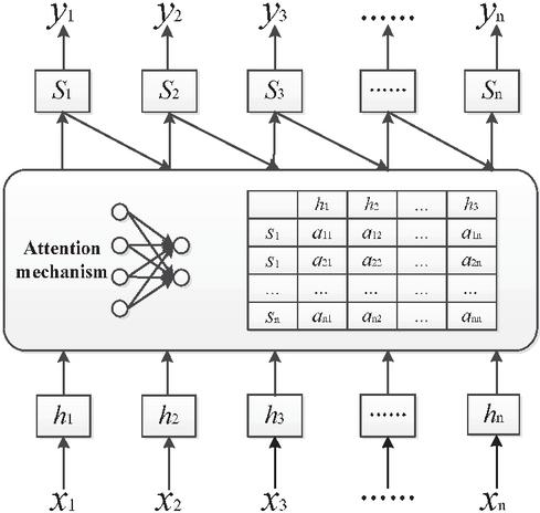
Figure 6 Structure of attention mechanism.
In Figure 6, after each input data is encoded, it will become a one-to-one corresponding encoder hidden state , and the attention module can automatically learn the weight . is used to reflect the correlation between the encoder’s hidden state and the decoder’s hidden state . The value of the intermediate semantic is obtained by the weighted sum of the hidden states of all encoders by the attention weight. Assuming that the number of input sequences is , the formula for calculating is:
| (8) |
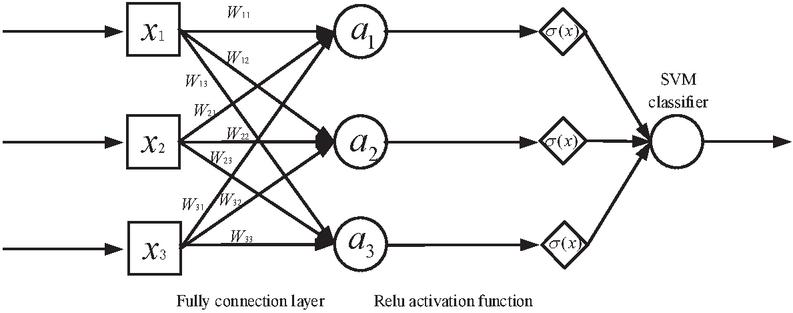
Figure 7 Schematic diagram of the full connection layer structure.
The attention mechanism adjusts the weight value of through continuous training of input data to improve the weight of feature words with a strong ability to distinguish categories for the purpose of improving an overall classification effect. In addition, by reducing the weight of unimportant feature words, the influence of unimportant information in the text can also be reduced. In text classification, more weights are assigned to feature words or sentences that have an impact on the distinction of text categories. Meanwhile, to those ones with not so many distinct features, less weight would be given.
3.2 SVM Classifier
To improve the performance of the CNN, the full connection layer selects the Relu function as the activation function. The most important function of the full-connection layer in the model is to play the role of “classifier”. The traditional CNN model combines the full-connection layer and Softmax layer to complete the classification. When the CNN model is used for text classification, the input data are nonlinear and sparse word vectors, so SVM has a better classification effect than the Softmax layer for this kind of data. Therefore, in the CNN-SVM model, the SVM classifier is used to replace the Softmax layer to achieve the final text classification. The full connection layer framework of the CNN-SVM model is shown in Figure 7. Figure 7 is a schematic diagram of the fully connected layer structure of the CNN-SVM model, in which each neuron is connected with the upper layer. The fully connected layer continuously updates the weight coefficient W through forward calculation and backpropagation to make the model reach the preset threshold. Using the Relu activation function in the full connection layer can improve the expression ability of a neural network to the model and solve the problem of linear indivisibility.
The SVM classifier has obvious advantages in solving the problems of small samples, nonlinearity, and high dimensions. The SVM classifier is featured with its ability to transform the low dimensional nonlinear feature space into high dimensional and linear feature space by using the kernel function [25].
As shown in Figure 8, the solid line in the figure is located between the two classification samples to separate two types of samples (represented by black and white dots). When there is noise in the training set, the hyperplane on this line is least influenced and the classification results will have the best robustness and the strongest generalization ability for non-appearing samples.

Figure 8 Schematic diagram of support vector machine.
In Figure 8, the hyperplane for classification is described by . Where is the normal vector, which represents the direction of the hyperplane; is the displacement, representing the distance between the hyperplane and the coordinate origin; is the transpose of the normal vector. According to the hyperplane formula, the distance from any point in the sample space to the hyperplane can be expressed as:
| (9) |
Let a given sample set be D, where any point is an element in the sample set , that is, , and represents two different categories respectively. If , i.e. , this means that belongs to the category represented by solid dots in Figure 4. If , i.e. , this means that belongs to the category represented by white dots in Figure 8. Combining the two formulas, we get:
| (10) |
In Figure 8, two dotted lines are used to represent the hyperplanes of the two boundaries in Equation (9). The sample set closest to the hyperplane satisfies Equation (10), that is, the support vectors will be on the dotted lines in Figure 8. If the distance between the hyperplane and the two different types of support vectors is set as and respectively, it is required that , that is, the two dotted lines should be equally distant from the solid line to ensure the strongest robustness. The specific calculation formula is:
| (11) |
Let , then . When reaches the maximum value, the hyperplane is the partition hyperplane with a “maximum interval”.
For the text classification model, the application scenario is for multi-category classification, which needs to solve the problem of linear indivisibility. Then, two variables, the relaxation variable, and the penalty factor would be introduced to increase the fault tolerance of the classification model. Therefore, the optimization condition formula is [26]:
| (12) |
where is the normal vector, which represents the direction of the hyperplane; is the displacement, representing the distance between the hyperplane and the coordinate origin; represents the corresponding category label; represents the constraint condition; and represents the square of the normal vector module.
Using the Lagrange multiplier method to construct the Lagrange function for Equation (11), we can get:
| (13) |
Where and are Lagrange operators. Let the partial derivative of to , , and be 0:
| (14) |
Substituting Equation (14) into Equation (3.2), the dual formula of Equation (12) can be obtained as follows:
| (15) |
By solving Equation (15), the optimal solution of the classification function can be obtained as follows:
| (16) |
where is called the kernel function. In this paper, the kernel function adopts the inner product kernel function, namely . The classification model based on a support vector machine uses different kernel functions to achieve better classification performance for nonlinear data.
4 Simulation and Analysis
4.1 Parameter Setting
(1) Word vector dimension
In the preprocessing stage, the text data set needs word vectorization. When the dimension of the word vector is too high, the operation time and running time of the system will increase. On the contrary, if it is too low, it can’t well reflect the approximate relationship and category differences between words, which affects the effect of text classification. For the Amazon Review Polarity Datasets used in this paper, when the word vector degree is increased from 64 to 128 dimensions, the precision is only slightly improved, as shown in Figure 9. So a 64-dimension of word vector is selected in this experiment.
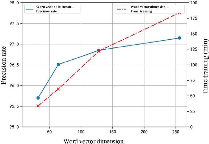
Figure 9 The determination of the word vector dimension.
(2) Text sequence length
The maximum sequence length that can be input into the model will also have a certain impact on its classification effect. If the maximal length of the text sequence is set too low, the model may not capture enough data features and thus reduce its precision; but if it is set too high, overfitting of the system, too long model training time or reduced and unstable precision will occur. Therefore, an optimal length of the text sequence should be adjusted to cater to the proposed CNN-SVM model. When text data is put into the CNN model for training, it is necessary to compare its length with the preset threshold. If it is greater than the preset threshold, it should be divided into subtexts. When it is less, it needs to be filled with space characters, as shown in Figure 10. In this experiment, the threshold of maximal text sequence of 600 is set.
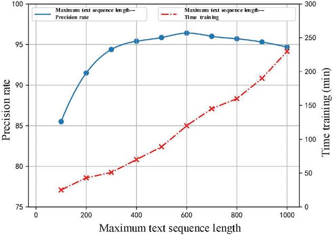
Figure 10 The determination of the maximum text sequence length.
(3) Other parameters in the model
In the process of constructing the CNN-SVM model, in addition to determining the dimension of the word vector and the maximum length of the text sequence input, many parameters need to be set in advance. In this experiment, the length of the convolution kernel is 5, the number of convolution kernels is 256, and the width of the convolution kernel is consistent with the dimension of the word vector, which is 64. The experiment uses the data set of Amazon Review Polarity Datasets from the Stanford Network Analysis Project, including the training set and test set. The specific distribution is shown in Table 1. The number of neurons in the whole connecting layer was 128. When using the training set for testing, the classification precision is very high, but when running a new data set, the classification effect is quite different.
| Class Alias | Training Set | Test Set | Proportion |
| underlineHappy | 680 | 680 | 8.5% |
| Excitement | 1340 | 1340 | 16.75% |
| Satisfaction | 1020 | 1020 | 12.75% |
| Calmness | 830 | 830 | 10.375% |
| Anxiety | 1250 | 1250 | 15.625% |
| Regret | 980 | 980 | 12.25% |
| Disgust | 740 | 740 | 9.25% |
| Anger | 1160 | 1160 | 14.5% |
| Total | 8000 | 8000 | 100% |
4.2 Experimental Results and Analysis
To evaluate the performance of the proposed algorithm, the CNN model [27], the TF-IDF model [28], and the proposed CNN-SVM model in this experiment are compared for handling the same data set. The experimental operation platform is the Windows 10 Professional operating system, with 16 GB memory and 2.8 GHz CPU. The main software environment is based on Python 3.6.7 and Pycharm 2018.12.5. The precision rate, recall rate, and value were analyzed as follows.

Figure 11 Comparison of precision rate.
(1) Precision rate
As can be seen from Figure 11, the classification precision of the CNN-SVM algorithm is higher than that of the CNN and the TF-IDF algorithm. With the increase in the amount of text in the training set, the precision of each classification model is also increasing. When the number of texts in the test sets reaches its maximum, the precision rates of the CNN-SVM model, CNN model, and TF-IDF model are 98.2%, 96.2%, and 85.4% respectively. Although the precision of the TF-IDF algorithm combined with a naive Bayesian classifier is improved, its precision is limited because the TF-IDF algorithm can’t give weight respectively according to the word location information but calculates the IDF value only by word frequency. The classification precision of the CNN model is not as good as that of the CNN-SVM yet better than the TF-IDF algorithm. The reason is that the classification model based on the CNN can extract the features of text more thoroughly, thus a better feature word vector can be obtained to improve the final effect of the classification model. Among the three algorithms, the proposed CNN-SVM model works best. That is because it adds an attention mechanism and simplifies the parameters based on the CNN model. Meanwhile, this model uses the classifier based on a support vector machine to replace the Softmax layer in the traditional model to improve precision.
(2) Recall rate
As can be seen from Figure 12, the recall rate of CNN-SVM is higher than that of the other two algorithms. The recall rate increase linearly as the number of texts in the data set increases. When the number of texts reaches its maximum, the recall rates of the CNN-SVM algorithm, CNN algorithm, and TF-IDF algorithm are 97.5%, 96.1%, and 79.6% respectively.
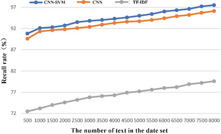
Figure 12 Comparison of recall rate.
(3) value
As shown in Figure 13, the value of the CNN-SVM model is higher than that of CNN and TF-IDF, which proves that the classification effect of the algorithm mentioned in this paper is the best.

Figure 13 Comparison of the F1 value.
From the three indicators of precision, recall, and value, the result of CNN-SVM is better than that of the CNN model and TF-IDF model. This shows that the effect of text classification based on the SVM classifier instead of the Softmax normalized exponential function is better.
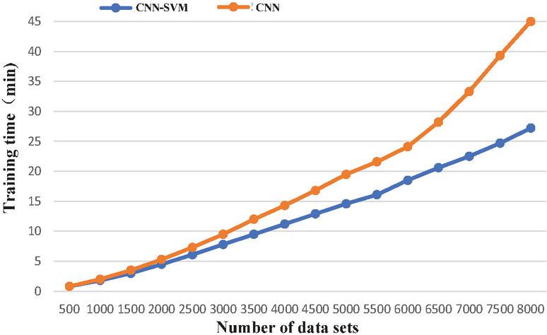
Figure 14 Comparison of model training time.
(4) Training time
Figure 14 shows the comparison of training time between the CNN-SVM model and the CNN model. The CNN-SVM model algorithm uses an SVM classifier to replace the Softmax normalized exponential function in the original model, so it can reduce the training time and improve the training efficiency. When the training set is small, the training time of the CNN-SVM model is not much improved compared with the CNN model, but with the increase in the amount of data, the improvement in the efficiency of CNN-SVM becomes more obvious.
Table 2 Comparison of error rates
| Amazon Review Polarity | TREC | Kaggle | ||||
| Short | Long | Short | Long | Short | Long | |
| Text | Text | Text | Text | Text | Text | |
| CNN-SVM | 5.29% | 5.86% | 5.25% | 5.88% | 5.24% | 5.85% |
| CNN | 5.58% | 6.1% | 5.61% | 6.15% | 5.63% | 6.18% |
| TF-IDF | 8.46% | 9.0% | 8.52% | 9.23% | 8.50% | 9.11% |
| RNN | 5.27% | 5.48% | 5.24% | 5.52% | 5.23% | 5.51% |
| BERT | 5.08% | 5.23% | 5.02% | 5.19% | 5.07% | 5. 25% |
Table 3 Comparison of training time
| Model Datasets | Amazon Review Polarity | TREC | Kaggle |
| CNN-SVM | 28 min | 31 min | 29 min |
| CNN | 45 min | 49 min | 47 min |
| TF-IDF | – | – | – |
| RNN | 63 min | 65 min | 68 min |
| BERT | 58 min | 61 min | 63 min |
(5) Comparative testing
To test the performance of the proposed algorithm, the error rates and training times of the proposed algorithm, CNN, TF-IDF, RNN, and BERT are compared based on Amazon review polarity, Text Retrieval Conference (TREC) and Kaggle datasets. Among them, TREC is from the Defense Advanced Research Projects Agency and the National Institute of Standards and Technology. Kaggle datasets is from Google. In the comparative experiments, samples are divided into short and long texts with a maximum of 255 tokens in short text and 8000 samples are trained. The comparative results are shown in Tables 2 and 3. From the tables, it can be seen that TF-IDF has the highest error rate in short text tasks, while other algorithms have similar error rates. In long text tasks, the proposed algorithm has a little bit higher error rate than RNN and BERT but shorter training time. The reason is that although CNN-SVM better extracts feature values, it does not fully consider the correlation of text context.
5 Conclusion
By combining the CNN model with the SVM classifier, this paper tries to make some fusion of the advantages of both with some inner modification: (1) the SVM is used to replace the normalization function in the CNN to realize text classification and to solve the problem of the insufficient generalization ability of the original model; (2) Compared with the CNN model, the CNN-SVM model is added with an attention mechanism. The function of this mechanism is to refine the feature words and select the feature words with stronger category representation to improve the precision of model classification. Through comparative experiments, the proposed algorithm has achieved better results in classification effect and training time. Despite the fine results, there are still many aspects to be optimized. For example, feature word vectors can be extracted through the CNN model and combined with more classifiers (like the logistic regressive, the K-nearest neighbor, etc.), then different combinations of models can be chosen according to application scenarios.
Acknowledgments
This project is supported by the Major Project of the National Social Science Foundation of China (18ZDA032)
References
[1] D. W. Otter, J. R. Medina, J. K. Kalita, “A survey of the usages of deep learning for natural language processing” IEEE Transactions on Neural Networks and Learning Systems, vol. 32, no. 2, pp. 604–624, 2021.
[2] H. Azarbonyad, M. Dehghani, M. Marx, et al., “Learning to rank for multi-label text classification: Combining different sources of information”, Natural Language Engineering, vol. 27, no. 1, pp. 89–111, 2021.
[3] W. F. Liu, J. M. Pang, N. Li, et. al., “Research on multi-label text classification method based on tALBERT-CNN”, International Journal of Computational Intelligence Systems, vol. 14, no. 1, 2022.
[4] K. M. Schneider, “A new feature selection score for multinomial naive bayes text classification based on kldivergence,” Proceedings of the ACL Interactive Poster and Demonstration Sessions, 2004, pp. 186-189.
[5] A. Z. Guo, Y. Tao, “Based on rough sets and the associated analysis of KNN text classification research”, International Symposium Distributed Computing and Applications Business Engineering and Science, 2015, pp. 485–488.
[6] Y. Chali, S. A. Hasan, “Query-focused multi-document summarization: automatic data annotations and supervised learning approaches”, Natural Language Engineering, vol. 18, pp. 109–145, 2012.
[7] G. G. Chowdhury, “Natural language processing. Annual review of information science and technology”, vol. 37, no. 1, pp. 51–89, 2003.
[8] Q. Li, H. Peng, J. Li, et al., “A text classification survey: from shallow to deep learning”, arXiv preprint arXiv:2008.00364, 2020.
[9] C. Cortes, V. Vapnik, “Supportvector networks”, Machine learning, vol. 20, no. 3, pp. 273-297, 1995.
[10] T. Joachims, “Text categorization with support vector machines: Learning with many relevant features”, European Conference on Machine Learning, 1998, pp. 137-142.
[11] J. H. Friedman, “Stochastic gradient boosting”, Computational Statistics and Data Analysis, vol. 38, no. 4, pp. 367-378, 2002.
[12] H. Wu, Y. Liu, J. Wang, “Review of text classification methods on deep learning. Computers Materials and Continua, vol. 63, pp. 1309-1321, 2020.
[13] O. Zennaki, N. Semmar, L. Besacier, “A neural approach for inducing multilingual resources and natural language processing tools for low-resource languages”, Natural Language Engineering, vol. 25, no. 1, pp. 43–67, 2019.
[14] G. Arevian, “Recurrent neural networks for robust realworld text classification”, IEEE/WIC/ACM International Conference on Web Intelligence (WI’07). IEEE, 2007, pp. 326-329.
[15] S. Hochreiter, J. Schmidhuber, “Long shortterm memory”, Neural Computation, vol. 9, no. 8, pp. 1735-1780, 1997.
[16] X. S. Yu, S. Shen, P. Chen, et al., “Electronic medical record classification method based on LSTM of text word features dimensionality reduction”, IEEE International Conference on Software Quality, Reliability and Security Companion, 2021, pp. 365–371.
[17] A. Vaswani, N. Shazeer, N. Parmar, et al., “Attention is all you need”, Advances in Neural Information Processing Systems, 2017, 30.
[18] W. Q. Gao, H. Huang, “A gating context-aware text classification model with BERT and graph convolutional networks”, Journal of Intelligent and Fuzzy Systems, 40(3), 4331–4343, 2021.
[19] N. Kalchbrenner, E. Grefenstette, P. Blunsom, “A convolutional neural network for modelling sentences”, Annual meeting of the Association for Computational Linguistics, 2014.
[20] Y. Chen, “Convolutional neural network for sentence classification”, University of Waterloo, 2015.
[21] W. J. Tao, D. Chang, “News text classification based on an improved convolutional neural network”, Tehnicki Vjesnik-Technical Gazette, vol. 26, no. 5, pp. 1400–1409, 2019.
[22] J. Peng, S. Q. Huo, “Few-shot text classification method based on feature optimization”, Journal of Web Engineering, vol. 22, no. 3, pp. 497–514, 2023.
[23] K.V. Raju, M. Sridhar, “Review-based sentiment prediction of rating using natural language processing sentence-level sentiment analysis with bag-of-words approach”, First International Conference on Sustainable Technologies for Computation Intelligence, 2020, pp. 807–821, 2020.
[24] N. I. Widiastuti, “Convolution neural network for text mining and natural language processing”, 2nd International Conference on Informatics, Engineering, Science, and Technology, 2019.
[25] I. Ali, N. Mughal, Z. H. Khand, et. al., “Resume classification system using natural language processing and machine learning techniques”, Mehran University Research Journal of Engineering and Technology, vol. 41, no. 1, pp. 65–79, 2022.
[26] Y. L. Gong, N. N. Lu, J. J. Zhang, “Application of deep learning fusion algorithm in natural language processing in emotional semantic analysis”, Concurrency and Computation-Practice and Experience, vol. 31, no. 10, 2019.
[27] Y. Li, X. J. Yang, M. Zuo, et. al., “Deep structured learning for natural language processing”, ACM Transactions on Asian and Low-resource Language Information Processing, vol. 20, no. 3, 2021.
[28] M. Madeja, J. Poruban, “Unit under test identification using natural language processing techniques”, Open Computer Science, vol. 11, no. 1, pp. 22–32, 2021.
Biographies
Jing Peng received her bachelor’s and master’s degrees in English language and literature respectively from Sichuan International Studies University in 2005 and Shanghai International Studies University in 2010. She is currently pursuing her Ph.D. degree in logic in the School of Philosophy, Anhui University. Her current research interests include natural language processing, fuzzy logic and artificial intelligence logic.

Shuquan Huo received his bachelor’s degree in foreign philosophy from Zhengzhou University, his master’s degree in foreign philosophy from Sun Yat-sen University and his doctorate degree from Nankai University, respectively. He is currently working at Henan University. His research areas include modern logic, philosophy of language, and philosophy of mind.
Journal of Web Engineering, Vol. 23_3, 315–340.
doi: 10.13052/jwe1540-9589.2331
© 2024 River Publishers