IaaS Cloud Adaptive Anomaly Detection Based on the DQN Algorithm
Li Chen*, Jia Xu and Fan Gou
Wuhan Wendao Information Technology Co., Ltd, Wuhan, 430000, China
E-mail: chenli8666@163.com
*Corresponding Author
Received 30 August 2024; Accepted 15 December 2025
Abstract
Aiming at the challenges of anomaly detection of virtual machine memory, network, CPU and hard disk in the IaaS cloud environment, this study proposes an adaptive anomaly detection system based on a deep Q-network. The system constructs a hierarchical detection framework: a spatio-temporal feature extraction module via fused temporal convolutional networks (TCN) for sequential pattern mining and convolutional neural networks (CNN) for cross-metric correlation learning; a transfer learning module to enhance generalization; and a deep Q-network (DQN) based central controller that dynamically adjusts detection parameters through reinforcement learning. This architecture integrates with cloud workload schedulers by operating at the VM-level (anomaly detection) and edge-server level (DQN control), minimizing core network overhead. Experiments show that the research method achieves a detection accuracy rate of 99.8% in the benchmark test, with an F1 score of 98.7%, which is significantly superior to the accuracy rate of 96.5% of the single convolutional neural network, 92.3% of the multi-layer perceptron, and 97.8% of Google Net. The transfer training experiments show that the accuracy rate of the untuned model on the new dataset is only 70% to 80%, while the detection accuracy can be stably improved to 98% through the adaptive system driven by the DQN. The system shows low volatility during the dynamic adjustment process. The number of training iterations is reduced by 32.3% to 69.8% compared with the traditional static model, indicating that the research method does not affect the time complexity. Research shows that this framework effectively solves the problem of insufficient adaptability of static models to unknown data in the cloud environment through the collaborative mechanism of spatio-temporal feature extraction and reinforcement learning decision-making, providing intelligent operation and maintenance solutions for fields with high reliability requirements such as finance and healthcare.
Keywords: Deep Q-network, abnormal detection, convolutional neural network, time convolutional network, cloud computing.
1 Introduction
Cloud computing (CC) refers to the use of network computing to store various resources and services in the cloud in the form of a network for users to obtain the necessary resources and services. It has the characteristics of dynamic expansion, on-demand deployment, resource sharing, virtualization, and so on. Since its inception, the industry scale of CC has been continuously expanding. The development trend of large-scale, distributed, and highly complex applications has made the architecture and service types of cloud systems increasingly complex and diverse. The frequency of system anomalies caused by this also continues to increase [1]. These exceptions can reduce the security and stability of cloud service systems, leading to data loss, downtime, or other more serious failures. This will affect the user experience and cause economic losses for cloud service providers. Therefore, it is necessary to adopt corresponding means to monitor and diagnose abnormal situations in the CC environment in real-time. There are many types of indicators that virtual machines can monitor in CC environments. It has a long monitoring time and a huge amount of monitoring data. It is difficult to timely identify potential faults solely by manual labor or traditional tools. Directly monitoring all indicators would also waste a lot of spatial resources. If artificial intelligence methods can be used to detect anomalies in key performance indicators in virtual machines, it will not only significantly reduce the amount of data monitored by the system, but also timely handle anomalies and reduce the occurrence of faults. At present, although anomaly detection methods based on traditional machine learning (such as isolated forests and support vector machines) can achieve high detection accuracy in static environments, they rely on manual feature engineering and have difficulty capturing the dynamic correlation of time series data [2]. In recent years, deep learning models have improved the detection effect through automatic feature extraction, but they still face two major challenges. First, model training relies on a large amount of labeled data, while abnormal samples are scarce and unevenly distributed in the cloud environment. Secondly, most of the existing methods are static models and cannot dynamically adjust parameters according to environmental changes, resulting in a significant decline in detection performance when there are sudden changes in heterogeneous resource loads or user behaviors of virtual machines [3]. For example, although the LSTM anomaly correction model proposed by Baghoussi et al. performs well in fixed scenarios, its accuracy rate drops by more than 20% when it is migrated to a new virtual machine environment [4]. The current commonly used anomaly detection (AD) method is used to train corresponding models by selecting appropriate algorithms based on historical data. However, this method exhibits poor performance in the face of new environments and data, requires manual intervention and regulation, and cannot achieve effective detection results. Based on this, the research proposes to introduce a reinforcement learning algorithm deep Q-network (DQN) into AD. This AD model has been automatically adjusted based on the current virtual machine operating environment and user usage habits. Therefore, AD accuracy can be improved in different scenarios and application scenarios. The model selection is justified by the problem’s specific demands. TCN is chosen over a long short-term memory/gated recurrent unit for its superior parallelization, efficient capture of long-range dependencies in time-series data, and stable gradient properties, which are crucial for real-time cloud monitoring. CNN is naturally suited for extracting spatial correlations across multi-dimensional metrics. For reinforcement learning, DQN is optimal because the action space is discrete and low-dimensional. Algorithms like DDPG are designed for continuous control, which would introduce unnecessary complexity for this task. DQN’s experience replay mechanism also ensures stable learning in the non-stationary cloud environment.
This research is mainly divided into four parts. The first part introduces the research status of the AD algorithm and the application progress of DQN, and proposes a new adaptive AD system to address the shortcomings of AD models. The second part explains in detail the application methods and processes of algorithms in recommendation models from three aspects: the overall architecture of adaptive AD systems, improved AD algorithms, and DQN adaptive decision-making construction. The third part conducts experimental verification and analysis on the improved AD algorithm and transfer training process, and tests the performance of DQN adaptive decision-making and the adaptive AD system. The fourth part summarizes the results of this study, analyzes its shortcomings, and proposes directions for improvement.
2 Related Works
The development of artificial intelligence has driven the improvement and expansion of deep learning (DL) technology, which has also demonstrated excellent performance in solving AD problems. Li et al. proposed a multi model feature fusion method based on DL for complex industrial process fault diagnosis. They extract effective features of different faults and obtain corresponding residual matrices. In the experiment, all features and residuals were concatenated as new inputs to establish a fault diagnosis classifier. Simulation experiments have shown that its performance and efficiency are both superior [5]. Liu et al. proposed a detection model based on an improved long short-term memory network around the detection and correction of IoT data. Experiments have shown that this model can not only reduce regression errors but also achieve real-time detection and correction of abnormal data in the Internet of Things, and improve the stability and robustness of the model [6]. The abnormal driving behavior detector has problems such as large labeled data, and it is time-consuming and labor-intensive. Hu et al. studied a DL based abnormal driving detection model. In the experiment, stacked sparse autoencoders were used to learn driving behavior features, and greedy algorithms were used for hierarchical training. Dropout technology was introduced during the training process to avoid overfitting of the model. This method is superior to the most advanced abnormal driving behavior detection technology [7]. Raichura et al. proposed a model that integrates convolutional neural networks (CNN) and extreme gradient boosting to improve the classification accuracy of internal faults in transformers. After extracting the features of the training data using one-dimensional CNN, the combined model is used to classify different internal and external faults of transformers. The simulation experiment shows that this method can correctly judge the operation status of transformers. Compared with existing machine learning methods such as vector machines, this method improves the accuracy of transformer internal fault recognition [8]. Xin et al. studied an anomaly network traffic detection model based on hybrid fuzzy integrated CNN, which is used to solve the problem of the identification of different tags with the same network traffic characteristic value that cannot be solved by previous algorithms. This method constructs an integrated algorithm based on the unique temporal characteristics of individuals with the same features. In the experiment, identical feature individuals with different labels will be converted into different feature individuals with different labels to achieve precise classification. Experiments have shown that this method performs better and more reliably than existing machine learning models [9]. DQN is a combination of a CNN and a Q-learning algorithm, with strong visual perception and learning decision-making ability, commonly used in the field of intelligent control. The integration mode of DL and Q-network is mainly reflected in approximating the Q-function through deep neural networks (DNN), thereby optimizing the strategy of reinforcement learning. In traditional Q-learning, Q-value functions are usually stored and updated using tables. However, when the state space and action space of the problem are very large, the table method is no longer applicable. To overcome this limitation, the Q-network adopts the DL model, especially the CNN or fully connected neural networks, to approximate the Q-value function through neural networks, thereby being able to handle more complex and large state spaces. This integration method has greatly expanded the application scope and effect of Q-learning, performing particularly well in high-dimensional problems. Quek et al. studied the control effect of the DQN algorithm on autonomous vehicles in 2D and 3D simulation environments. In these two simulation environments, autonomous vehicles can learn manipulation through training, navigate without prior information, and control the vehicle to avoid obstacles [10]. Zheng et al. studied a linear active disturbance rejection control method based on the DQN algorithm for load frequency control in multi-area interconnected power systems. This method takes the output of the power system as the environmental state in the DQN, takes the parameters of the controller as the actions in the DQN, and improves the action selection strategy and reward function. This method is better and more stable than the proportional integral differential controller with fixed parameters and the linear active disturbance rejection controller without introducing the DQN algorithm [11]. Mei et al. proposed an intelligent radio access network fragmentation strategy with two-layer control granularity. The upper controller can perform adaptive slicing configuration for loose control based on the long-term dynamic execution of service traffic. The lower level controller is integrated through deep deterministic strategy gradient and dual DQN algorithm collaboration. It can improve the long-term service quality and spectral efficiency of the partition. This method has been proven to be effective and has superior performance [12]. Ke et al. proposed a dual DQN based variable speed limit control strategy to enhance the transferability of variable speed limit control. It can transfer the knowledge learned from the source scene to other target scenes. Compared with variable speed limit control without the introduction of DDQN, the training process has been reduced by 32.3–69.8%. It has been proven that this strategy has good transferability [13]. Bommes et al. trained ResNet-34 convolutional neural networks with supervised contrast loss and used a k-nearest neighbor classifier to detect anomalies. On a target dataset containing 2.92 million infrared images, this method achieved an area under the receiver operating characteristic curve ranging from 73.3% to 96.6%, and its performance was superior to that of classifiers based on binary cross-entropy. At a fixed decision threshold, this resulted in 79.4% and 77.1% of the images being correctly classified as normal and abnormal images, respectively. Experimental results show that the proposed method is insensitive to hyperparameter setting, converges quickly, and reliably detects unknown types of anomalies, ideal for practice [14]. Kate et al. proposed a novel method to further characterize these abnormal images, using a convolutional autoencoder to reduce the dimensionality of the residual difference between real and WGAN reconstructed images and perform UMAP clustering on these images. The reported anomalies including galaxy mergers, tidal signatures, and extreme star-forming galaxies are reported. This was found to be an unusual system with a very blue, higher metallicity II region [15].
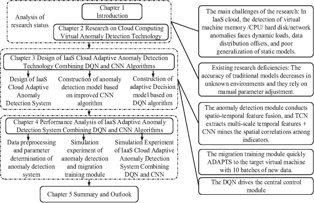
Figure 1 Technology roadmap of this paper.
In summary, existing research has confirmed the effectiveness and potential of deep learning in anomaly detection feature extraction. However, the research of Mei et al. and Ke et al. focuses on resource allocation optimization in specific fields such as network slicing and traffic control, and the design of their state space and reward functions is not intended to directly optimize the performance of anomaly detection models. Aiming at the problem of poor performance of a single convolutional neural network in detecting anomalies in unfamiliar data, this study proposes an adaptive anomaly detection system based on a DQN model, combined with a temporal convolutional network (TCN) and a CNN. Compared with other recent works, the innovation of the proposed method lies in the construction of an end-to-end adaptive anomaly detection framework. The core of this framework is to directly use the accuracy, loss, and resource overhead of anomaly detection models as the state and reward inputs for deep reinforcement learning. Through this approach, DQNs are specifically used to dynamically adjust the parameters of detection models to achieve adaptive optimization of unknown data distributions. The advantage of this method is that it achieves real-time and automatic matching between detection strategies and dynamic environments, significantly improving the model’s generalization ability. The potential drawback is that its system structure is relatively complex, and the training and convergence of DQN agents depend on a certain amount of initial interaction data, which may result in a brief performance fluctuation period in the early stages of system deployment. The overall content structure of the article is shown in Figure 1. The first and second chapters (sections) analyze and describe the research status respectively. The third chapter is the design of IaaS cloud adaptive anomaly detection technology combining DQN and CNN, including the overall framework design of IaaS cloud adaptive anomaly detection system, the overall framework design of the anomaly detection system based on the improved CNN algorithm, and the construction of an adaptive decision model based on the DQN algorithm. The fourth chapter is the performance evaluation of an IaaS cloud adaptive anomaly detection system combined with DQN and CNN, including simulation experiment results of data preprocessing and parameter determination of the adaptive anomaly detection system, simulation results of anomaly detection and migration training module, and simulation experiment analysis of IaaS cloud adaptive anomaly detection system combined with the DQN and CNN. The fifth chapter is the summary and the prospect.
3 IAAS Cloud Adaptive AD Technology Combining DQN and CNN
Memory exceptions are a common type of failure in IaaS cloud system virtual machines. They may be caused by application memory leak, computer virus infection and other reasons. It not only leads to abnormal memory usage but also causes abnormal changes in other indicators such as a central processing unit (CPU), disks, and networks [16]. This study focuses on the abnormal performance of four key indicators: memory, network, CPU, and hard disk. An adaptive AD system is designed by using improved CNN and reinforcement learning algorithms to realize the adaptive detection of various anomalies in different virtual machines of the IaaS cloud.
3.1 Overall Framework Design for the IAAS Cloud Adaptive AD System
Human learning mainly relies on synaptic connections between neurons. Neural networks (NNs) can emulate the analysis, storage, and processing mechanisms of neurons for stimulus signals, and intelligently process information. Artificial NNs can learn the representation of user’s normal behavior mode from the existing information through repeated training, and judge the outlier based on this. Therefore, it is often studied and used in diagnostic systems for various abnormal data [17]. Cloud based virtual machine AD is one research direction [18]. Although there have been some research achievements in AD in the CC environment, most of the research has been on the foundation of models trained from a large amount of sample data in the past. Even if the NN has strong learning ability, it is more inclined towards AD in known environments. The recognition ability will decrease when facing abnormal situations in unknown environments [19–22]. This study proposes an IaaS cloud adaptive AD system that combines an improved CNN based AD module and a DQN based central control module. This method can improve the detection accuracy of the model for unknown different monitoring data sources, while solving the problem of abnormal data detection in IaaS cloud virtual machines. Figure 2 shows the structure of the system.
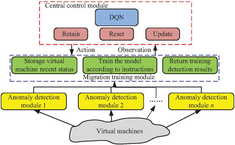
Figure 2 IaaS cloud adaptive AD system architecture.
As shown in Figure 2, the detection system can be divided into three parts: abnormality detection module, transfer training module and central control module. The anomaly detection module installed on the target virtual machine continuously collects the raw monitoring data of memory, network, CPU, and hard disk. This module preprocesses the data and inputs it into its internal model for real-time anomaly detection. The detection results and the original monitoring data are uploaded to the migration training module located on the edge server. The central control module receives information from the migration training module. The DQN agent builds the current environment state based on this information and predefined reward functions. Subsequently, the DQN agent makes a decision based on the -greedy strategy, choosing to perform an operation: keeping the model parameters unchanged, using a small batch of data for incremental updates, or performing parameter resets. After the action is executed, the system calculates the immediate reward through the predefined reward function based on the detection performance and resource consumption in the next time step. This interaction experience is stored in the experience replay pool of the DQN. The DQN agent samples batch data from the experience pool regularly and uses the Adam optimizer to minimize the temporal difference error to update the parameters of its valuation network, thereby learning the optimal action selection strategy. The training method of the model is divided into two stages, namely the centralized pre-training stage and the online adaptation stage after deployment. During the centralized pre-training phase, before deployment, the detection model is trained offline using a large-scale historical monitoring dataset to learn universal spatiotemporal feature representations. After system deployment, the online adaptation phase enters an adaptive loop centered around the DQN. The conditions for triggering online fine-tuning include periodic triggering and performance driven triggering. The DQN decision process is initiated for every N batches of monitoring data accumulated by the migration training module for the target virtual machine. When the real-time accuracy of the anomaly detection module remains below the preset threshold or the loss function value significantly increases, the DQN decision is immediately activated.
The anomaly detection module deployed on the target virtual machine continuously collects the raw monitoring data streams of the memory, network, CPU, and hard disk. This module first preprocesses the input data and then inputs it into its internally integrated model for real-time analysis. Based on the learned spatio-temporal feature patterns, the model performs classification tasks on the input monitoring data fragments and outputs the determination result of whether the current virtual machine operation status is abnormal [23–25]. Due to the huge number of IaaS cloud virtual machines, the subtle performance gap of each virtual machine also occupies part of the system space, so the exception detection module installed on the virtual machine needs to take into account the system space consumption and detection accuracy. The transfer training module is in the node position of the edge server near the virtual machine, and the transfer learning is the most core idea in the transfer training module, which is mainly designed to realize the rapid learning of the target virtual data characteristics by the module. In this study, the existing data is used to train the model and deploy the pre-trained model to the transfer training module, so that the model can learn enough features in the pre-training, and, in the face of a specific target virtual machine, under a small amount of data, quickly learn the data characteristics of the new environment, so as to adapt the model to the application environment. The definition of the domain in transfer learning is shown in Equation (1).
| (1) |
In Equation (1), represents the feature space and represents the edge probability distribution. In the detection system of this paper, exception detection in different user modes and virtual machine environment can be regarded as a problem in the same field. The definition of tasks in transfer learning is shown in Equation (2).
| (2) |
In Equation (2), represents the label space, and represents the target prediction function. This task is a certain task in the same field, and the training data is used to train the anomaly detection model. In the detection system, the main task of the central control module is to calculate the reward value of the state parameters and the abnormal detection results output by the reinforcement learning algorithm according to the set reward function, so as to achieve the purpose of adaptive abnormality detection and adjustment through the way of rewards and punishments. Pre-trained models are usually initially trained on a large-scale dataset and are capable of capturing common features in the data. In a Q-network, the pre-trained model can provide a powerful initialization to help accelerate the learning process. Specifically, the pre-trained model can provide a relatively robust strategy in the early stage of training, reducing the time and computational cost of learning from scratch through transfer learning. In addition, pre-trained models can also avoid overfitting in complex tasks, especially when there is insufficient data, providing more robust generalization capabilities. During the training process of Q-learning, by using the pre-trained model, the information in the dataset can be utilized more effectively, enabling the model to perform better when facing unknown environments.
3.2 Construction of an AD Model Based on an Improved CNN
Virtual machine memory exception is a common kind of abnormal memory. When the cause and environment are different, the CPU, hard disk and other related performance indicators in the virtual machine will also change accordingly. Deep learning networks identify these anomalies by learning the unique data features when they occur. If various deep learning algorithms are directly used to classify abnormal data points, this often leads to excessive system resource occupation and poor detection effect. Therefore, slicing the monitored data from the time series to detect the running status of the virtual machine and abnormal data types over a period of time is considered, which can not only reduce the resource consumption of the system, but also improve the accuracy of anomaly detection [26]. Therefore, based on TCN and CNN models, the Zoom-CNN anomaly detection model is proposed to improve the detection performance. This model is composed of a Zoom layer, a CNN convolutional layer, and a fully connected layer to realize the classification output. Its network model for the detection of anomalous time series data is shown in Figure 3.
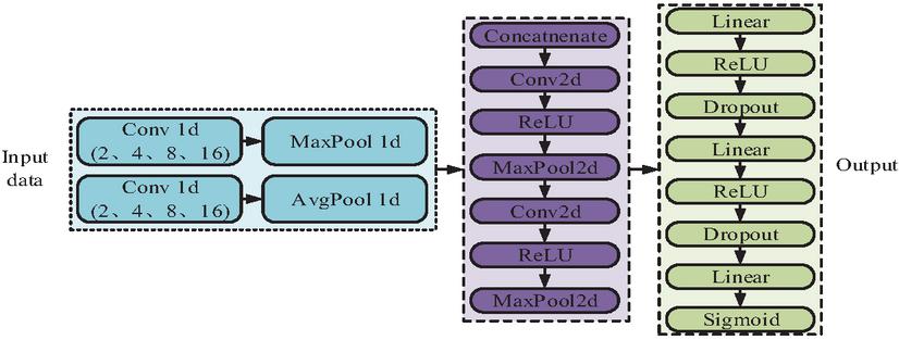
Figure 3 Network model for anomalous time-series data detection.
Through this anomaly detection model, only the CPU, memory, hard disk, and network monitoring data can be used to realize the comprehensive anomaly detection of the virtual machine time series data, without occupying the resources of the computing system. In this anomaly detection model, the Zoom layer in the first part is designed according to the convolutional neural network TCN to realize the extraction of time features in multiple dimensions of each monitoring number such as CPU and memory [27]. On this basis, the original monitoring data is expanded through multiple channels and its high latitude characteristics are mined. The input feature of the network is , and the expression of the component input vector is shown in Equation (3).
| (3) |
Vector passes through a hidden layer and, under the activation function, makes the intermediate output more diverse and handles more complex problems to achieve the nonlinear output. In this model, three activation functions are used, first, the Sigmoid function, which is monotonically increasing and is often used for the output of hidden layer neurons, mapping the final output between 0 and 1. The definition is shown in Equation (4).
| (4) |
The second is the tanh function, which aims to solve the zero-centered output problem and improve the convergence rate of the model. The definition is shown in Equation (5).
| (5) |
Another is the ReLU function, which is simple to calculate, converges faster, and can deal with the problem of gradient disappearance. In the Zoom-CNN model proposed in this study, the activation function used is the ReLU function. The definition is shown in Equation (6).
| (6) |
Through the final output result of the neural network, the classification task is realized, and the scope of the output results is defined as Equation (7).
| (7) |
Deep neural networks have good representation effect and can be used as a baseline in various tasks. In this study, a multi-layer perceptron with three linear layers can be used as the baseline for the anomaly detection model. The second part of the anomaly detection model is to realize the extraction of correlation features between different performance indicators, CPU utilization, hard disk use, network throughput, and memory utilization through the CNN model. The CNN model is a feedforward neural network, including a convolution layer and a pooling layer. It extracts the characteristics of each monitoring index in a certain time through convolution kernel, so as to realize the detection of anomaly. The process of the model implementing convolution and pooling is shown in Figure 4.
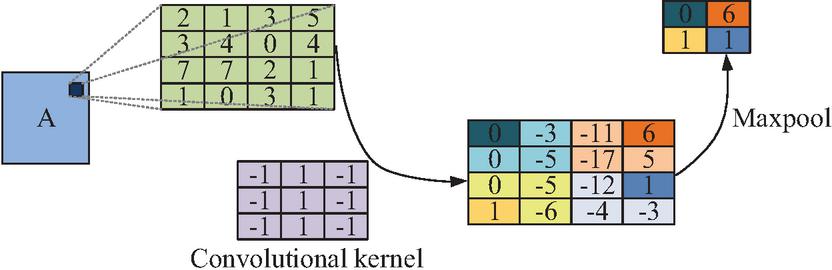
Figure 4 The CNN realizes the convolution and pooling process.
In the CNN model, the convolution kernel makes the matrix multiplication sum of the input features in turn and finally realizes the output of the results by combining with the deviation amount, and extracts the correlation features between the hard disk, memory, CPU and the network performance index of the virtual machine. The pooling layer is to further filter the output correlation features. By sampling the maximum or average features in the region, the size of the model can be reduced, the calculation speed can be accelerated, and the robustness of the model can be enhanced. The final result is achieved through three fully connected layers, so the third part of the anomaly detection model is the fully connected layer. The feature input of the convolutional layer is processed by using the maximum pooling and ReLU function to realize the classification of anomalies [28, 29]. The anomaly detection model enables fast and efficient anomaly detection of time series data of virtual machines. To prevent overfitting of the model during training and enhance its generalization ability on unknown data, this model introduces multiple regularization strategies. Firstly, the Dropout technique was applied in the fully connected layer. During the forward propagation process, some neurons were randomly discarded with a preset probability (set to 0.5 in the experiment) to reduce the complex co-adaptive relationships among neurons. Secondly, L2 weight attenuation (with a coefficient set to 0.0001) was added to the optimizer configuration to constrain the complexity of the model by imposing penalties on its weights. Furthermore, the Z-score standardization, as mentioned earlier, was also adopted in the training data preparation stage, which itself helps to stabilize the training process. These regularization measures work together to ensure that the model captures key spatiotemporal features without overly relying on specific noises or patterns in the training set.
3.3 Construction of an Adaptive Decision Model Based on the DQN Algorithm
The central control module uses the DQN algorithm to intelligently adjust the parameters of the IaaS cloud virtual machine AD model. The modules in DQN that make learning and decision-making are called agents. Intelligent agents change the state of the environment through policies. The environment will generate corresponding reward feedback. Based on the reward value, the intelligent agent can estimate the value of each action in a certain state, and then map the value estimation to the state action using a function constructed by NNs. The interaction between the environment and the state policy in the DQN algorithm can be described through Markov decision processes (MDPs) [30] in Equation (8).
| (8) |
is a set of specific states at a certain time, that is, the virtual machine timing data and detection results output by the migration training module. represents the actions taken by the migration training module at a certain time, including resetting, updating, and retaining the NN parameters of the corresponding AD module. represents the transition probability matrix, which is the probability of transitioning from action to the next state under state , and can be represented by Equation (9).
| (9) |
In DQN, is related to each action’s value estimation, and a fixed probability threshold can be set to select actions within a specific probability range to improve the algorithm’s computational efficiency. is a reward function that represents the reward value of the action taken by agent in state . The reward function plays a decisive role in the DQN, and the agent needs to learn the optimal strategy from the accumulated reward values [31, 32]. The accuracy reward is represented by Equation (10).
| (10) |
In Equation (10), and are the correctly predicted samples, while represents all samples of the batch. The accuracy rate is expressed as the sample proportion with correct prediction results to all samples. The higher the accuracy rate, the better the detection effect. The loss value represents the error between the predicted and true values. The smaller the loss value, the better the detection effect. Equation (11) calculates the reward value DD of loss.
| (11) |
is the loss function. The compression value of the virtual machine is related to the amount of data output in the network model. The input data volume for this study is 64 4 and 32 data samples are output per batch. After standardizing the data volume, its value ranges from 3 to 3. The smaller the compression value, the less resource space the model occupies, which can to some extent reduce the probability of serious consequences caused by memory anomalies. The reward of the compressed value is calculated using Equation (12).
| (12) |
In Equation (12), means the data batch, is the data length, represents the data dimension, and is a variable of these three mathematical quantities. Equation (13) is the final reward function.
| (13) |
The design of the reward function aims to balance detection accuracy and resource utilization. Among them, accuracy rewards are prioritized, ensuring detection performance, loss rewards encourage model convergence, and compression value rewards constrain model complexity to reduce resource consumption. Realize a balanced optimization with precision as the main focus and resources as the auxiliary through weight coefficients. The reward shaping mechanism provides additional positive rewards for behaviors that continuously improve accuracy or significantly reduce resource consumption in order to encourage strategies that steadily improve performance. To ensure the stability of learning, the system adopts three key mechanisms: experience replay is used to break the correlation between data; the target network is used to stabilize the update target of the Q value; the exploration rate linearly decays from 1.0 to 0.1 to balance exploration and utilization. These mechanisms collectively ensure the stable convergence of the DQN in non-stationary cloud environments. The reward function should not only consider the rewards generated by subsequent actions in Markov decision-making, but also avoid its significant impact on the current action reward. Therefore, it is necessary to introduce a discount factor for future action rewards, namely the discount rate . If there are actions in the entire process, Equation (14) is the cumulative reward obtained by an intelligent agent at moment .
| (14) |
In the equation, means the th action in the future. The DQN randomly selects action based on the transition probability. After performing this action, the reward can be obtained. The interactive data of environmental actions was placed in the experience pool. The valuation network can estimate the action value based on reward in the experience pool. Then the loss function in the NN is optimized by the Adam algorithm. The weight parameters of the valuation network are adjusted and updated through backpropagation [33]. After multiple training sessions, the optimal parameters were obtained. Figure 5 shows the structure and operational process of the DQN.
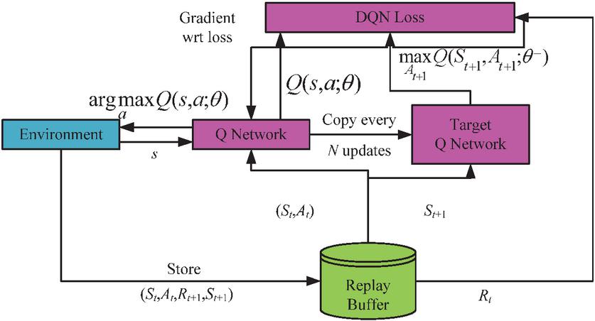
Figure 5 Structure and operation process of the DQN.
Each action output by the DQN directly affects the parameter update strategy of the anomaly detection module. Keeping the weights of the current TCN-CNN model unchanged without any updates is suitable for situations where the current model performs stably in the target environment. We fine tune the TCN-CNN model using the last 20 batches of monitoring data cached in the transfer training module and update the network weights through backpropagation to adapt to the local feature changes of the target virtual machine. Resetting the weights of the TCN-CNN model to the initial parameters of the pre-training stage is suitable for situations where the current model experiences severe performance degradation or overfitting in the target environment, and restoring the model’s generalization ability through reinitialization.
The adaptive anomaly detection system designed for research integrates TCN, CNN, and DQN modules through a layered architecture. The temporal feature extraction module adopts a multi-core parallel TCN structure, using four one-dimensional convolutional layers (kernel sizes of 2, 4, 8, and 16, with 32 channels) to process the monitoring indicator sequence, in order to capture multi-scale temporal dependencies. The output features of the TCN are concatenated in the channel dimension and used as inputs to the CNN module for learning memory CPU. The output features of the TCN are concatenated along the channel dimension and serve as input to the CNN module, aiming to learn and memorize CPU information. This module is designed to learn the spatial correlations between memory and CPU, as well as between hard disk and network metrics. The CNN consists of two layers of convolution (3 3 kernels, 64/128 channels), followed by ReLU activation and 2 2 max pooling layers, and finally the fully connected layer outputs the classification results. The detection model uses the Adam optimizer (learning rate 0.001) and cross entropy loss function to train 500 rounds with a batch size of 64. The DQN controller takes detection performance indicators as state inputs, and the action space includes three strategies: parameter maintenance, small batch update, and reset. Its network structure is a fully connected network of 64-128-64-3, trained using experience replay (buffer 50000) and target network (updated every 100 steps) mechanisms, with a discount factor of 0.99 and a linear decay of exploration rate from 1.0 to 0.1. The system utilizes TCN-CNN for feature extraction and classification, and the DQN dynamically adjusts the detection model parameters based on real-time performance to enhance adaptability to unknown environments.
The CNN part contains two layers of convolution operations, with a kernel size of 3 3 and the number of channels being 64 and 128 respectively. The pooling layer adopts the maximum pooling algorithm, and the window size is 2 2. The fully connected part is designed as a two-layer structure, with the number of neurons being 256 and 128 respectively. In terms of activation functions, the hidden layer uses the ReLU function, and the output layer adopts the Softmax function for classification. The optimizer selects the Adam algorithm, sets the learning rate to 0.001, and introduces a weight attenuation coefficient of 0.0001 to suppress overfitting. The loss function adopts cross-entropy loss, the batch size is fixed at 64, and the training period is 500 epochs. The configuration parameters used in the deep learning techniques are shown in Table 1.
Table 1 The configuration parameters used in the deep learning techniques
| Parameter | Value | Description |
| Learning rate | 0.001 | Learning rate used with the Adam optimizer. |
| Batch size | 64 | Number of samples per iteration. |
| Optimizer | Adam | Optimizer used for training. |
| Network architecture | Fully connected (3 hidden layers) | The structure of the neural network. |
| Activation function | ReLU | Activation function used in each layer. |
| Training epochs | 100 | Total number of training epochs. |
| Weight initialization | Xavier initialization | Method for initializing weights. |
| Loss function | Mean squared error (MSE) | Loss function used for the model. |
| Dropout rate | 0.5 | Dropout rate to prevent overfitting. |
| Data augmentation | Random cropping and rotation | Techniques to enhance training data variability. |
The pseudo-code of the proposed method in the research is specifically shown in Table 2.
Table 2 Research method: Pseudocode
| Algorithm 1: TCN-CNN-DQN for adaptive anomaly detection in the IaaS cloud | |
| Input: Historical monitoring dataset D_{pre} for pre-training Real-time monitoring streams from target VMs DQN hyperparameters: discount factor \gamma, replay buffer size B, exploration rate \epsilon, etc. Output: Adaptive anomaly detection decisions in real-time Procedure: // Phase 1: Centralized Pre-training Initialize TCN-CNN detection model M_{det} with random weights \theta for epoch = 1 to E_{pre} do Sample batch (X, y) \sim D_{pre} \hat{y} = M_{det}(X; \theta) // Forward pass Compute loss \mathcal{L} = \text{CrossEntropy}(\hat{y}, y) Update \theta via Adam optimizer if validation loss stops improving for P epochs then Break // Early stopping end if end for Save pre-trained weights \theta_{pre} // Phase 2: Online Adaptation with DQN Controller Initialize DQN agent with: - Online network Q(s, a; \phi) - Target network Q’(s, a; \phi∧-) with \phi∧- \leftarrow \phi - Replay buffer R of capacity B Deploy M_{det} with \theta \leftarrow | \theta_{pre} on target VMs for each time step t do Collect monitoring metrics x_t from VMs \hat{y}_t = M_{det}(x_t; \theta) // Real-time anomaly detection Compute detection accuracy acc_t, loss loss_t Construct state s_t = [acc_t, loss_t, \text{compression}_t] // DQN Action Selection With probability \epsilon select random action a_t Otherwise select a_t = \arg\max_a Q(s_t, a; \phi) Execute action a_t: if a_t = 0: Maintain current \theta if a_t = 1: Fine-tune \theta using recent N batches if a_t = 2: Reset \theta \leftarrow \theta_{pre} Observe new state s_{t+1} and compute reward r_t Store transition (s_t, a_t, r_t, s_{t+1}) in R // DQN Training Sample random minibatch (s_j, a_j, r_j, s_{j+1}) \sim R Compute target: y_j = r_j + \gamma \max_{a’} Q’(s_{j+1}, a’; \phi∧-) Update \phi by minimizing (y_j - Q(s_j, a_j; \phi))∧2 Every C steps update target network: \phi∧- \leftarrow \phi Decay exploration rate \epsilon end for |
4 Performance Evaluation of the IaaS Cloud Adaptive AD System Combining the DQN and CNN
In the performance evaluation, the fault generator is used to make exceptions, and the original data is artificially obtained and preprocessed. By using accuracy as an evaluation indicator, the accuracy of AD module detection, the effectiveness of transfer training module, and the application effect of adaptive detection system were verified through comparative experiments.
4.1 Adaptive AD System Data Preprocessing and Parameter Determination
IaaS cloud VM monitors four index data including memory, network, CPU and hard disk, and uses a software probe to sample and record its running state at interval, thus obtaining multi-dimensional performance index data flow. In addition, experiments employed a fault generator to inject faults into the virtual machines at random, based on six predefined scenarios: (1) ordinary memory leakage, (2) memory leakage and CPU abnormal occur at the same time, (3) memory leakage and hard disk abnormal occurs at the same time, (4) memory leakage and network abnormalities occur at the same time, (5) memory leakage and other three abnormalities occur at the same time, (6) virtual machine normal operation. The relevant parameters of the experimental environment configuration of this study experiment are shown in Table 3.
Table 3 Experimental environment configuration parameters
| Processor | Intel(R) Core(TM) i5-10600KF |
| Memory | 48G |
| Graphics card | Nvidia GeForce RTX 3070Ti |
| EDITOR | Jupyter notebook |
| Development language | Python 3.8.5 |
| Deep learning framework | Python 1.10.1 |
| Experimental physics server | |
| CPU | Intel(R) Xeon(R) CPU E5-2407 |
| 2.20Hz 4 cores and 4 threads | |
| Physical memory | 96G |
| Physical hard drive | 2T |
| Operating system | Centos7.5 |
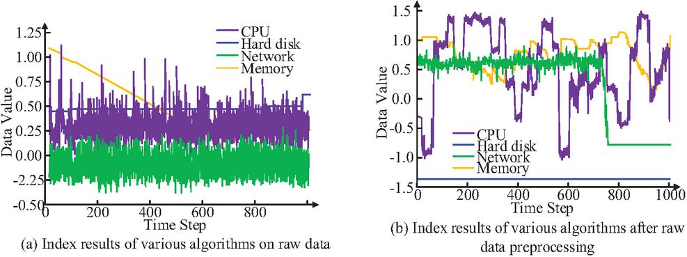
Figure 6 Partial data after standardized preprocessing (verifying the effectiveness of the Z-score method for the unification of multiple index dimensions).
The experimental data were collected through the monitoring agent deployed in the IaaS cloud virtual machine, mainly including four types of indicators: memory free space, CPU utilization rate, hard disk utilization rate, and network throughput. Prometheus v2.30 was adopted as the monitoring platform, combined with Node Exporter v1.3.1 to continuously collect data at a frequency of once per second for 14 days, and the total amount of original data reached 1.2 TB. To simulate real abnormal scenarios, the research developed a fault generation script based on Python 3.9 and injected exceptions into six scenarios: Common memory leaks are achieved by looped allocation of unreleased memory, and the leak rate is fixed at 100MB/s. CPU anomalies are triggered by high-load computing tasks, and the utilization rate is stable at over 95%. The hard disk anomaly uses the dd command to write random data blocks at a rate of 1 GB/s. Network anomalies are simulated by limiting the bandwidth to 10 Mbps and injecting a 20% packet loss rate. Each type of exception lasts for 30 minutes, with normal operation data such as file transfer and database query inserted during the intervals to be close to the real load. However, before calculation, it is necessary to standardize the data values to avoid significant differences in data values due to different data collection standards and measurement units. The standardization method uses the Z-score standardization method, and the normalized value is the difference between the value and the category it belongs to divided by the standard deviation. The reason for choosing the Z-score standardization method is that the dimensional differences of different monitoring indicators will cause the model training to be biased towards features with a larger numerical range. The standardized data distribution is closer to the normal distribution and can reduce the oscillation during the gradient descent process. The raw data is converted into various performance indicators in the virtual machine configuration, and the data results before and after standardization preprocessing are shown in Figure 6.
After data preprocessing, the data is divided into 5 minutes as a sequence batch, and each sequence batch is sliced with 64 data points per cycle. To provide reference for model training, the proportion of various data samples needs to be coordinated, and the gap should not be too large. Therefore, random sampling should be conducted on normal samples with a large amount of data and normal data with low usage rates of all indicators should be eliminated. Figure 7 shows the number and proportion of data after final screening.
According to Figure 7, the sample size and proportion distribution of each type of data are relatively balanced, and the difference is not significant, which can meet the experimental requirements. Randomly divide the processed data into a training set and a testing set in an 8:2 ratio for model training.
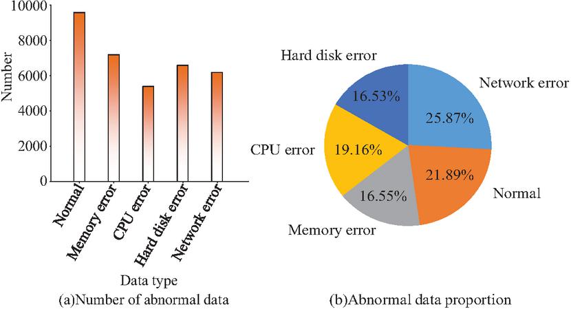
Figure 7 Distribution of the number and proportions of the different data types after the slice (showing the sample balance between abnormal types and normal data, verifying the rationality of experimental data and the fairness of model training).
4.2 Simulation Experimental Results of AD and the Transfer Training Module
Zoom layers with different kernel sizes are used to extract different features of time series data, so in this paper, Zoom layers with different kernel sizes are used to extract the effect of time features and compare the experiment. In the Zoom layer with different kernel sizes, after extracting features, the full connected layer is directly used for classification, and the experimental results of classification detection are shown in Figure 8.
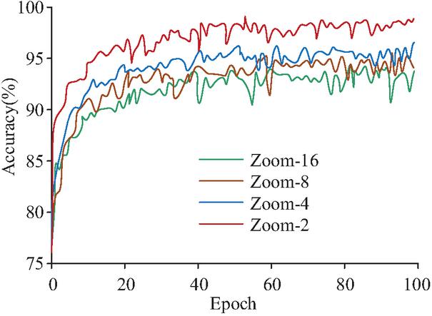
Figure 8 Effect of different convolution kernel sizes on model classification accuracy (analyzing the influence of different convolution kernel sizes on temporal feature extraction and verifying the advantage of small-sized convolution kernels in preserving local information).
According to Figure 8, the Zoom layer with a convolution kernel of size of 2 has the highest classification accuracy of 96.8%. Next is the Zoom layer with convolution kernel size 4, with a classification accuracy of 94.3%. Zoom layers with convolution kernel sizes 8 and 16 had low classification accuracy, with 92.1% and 91.8%, respectively. This indicates that the smaller the convolution kernel size set, the better the Zoom layer performs on the feature extraction of the time series. The reason for this analysis may be that the Zoom layer with large convolution core can extract earlier time dimension features, but it will also lose some local information, which reduces the classification accuracy. The test result data of the influence of different convolution kernel sizes on the classification accuracy of the model all have significant statistical significance. Overall, although the output accuracy of the Zoom layer with different convolution kernel sizes varies, it is above 90%, indicating that the structure can extract the temporal characteristics of the experimental data. In order to retain the temporal features of different original data at different scales, the features output by Zoom layer are spliced, and then input to the CNN layer for convolution pooling to extract the correlation features among the four types of data. Finally, output the classification results from the fully connected layer. The accuracy and loss function value of the whole anomaly detection module were analyzed and the MLP model was selected for the comparison experiment. In this experiment, the anomaly detection parameters of the model are set as follows: the number of network layers is 4, the connection type is linear, the activation function is ReLU/Dropout, and the output data is 128. The results are shown in Figure 9.
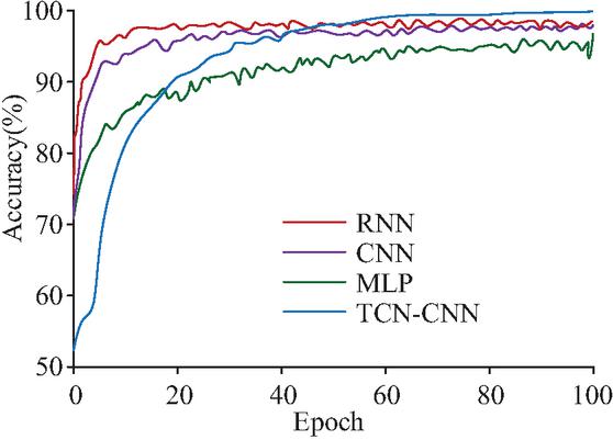
Figure 9 The detection accuracy of anomaly detection modules of different algorithms (comparing the detection accuracy and convergence speed of TCN-CNN, RNN, CNN, and MLP, highlighting the superior performance of the TCN-CNN model).
Figure 9 compares the anomaly detection accuracy and loss function values of four models (TDN-CNN, RNN, CNN, and MLP). The study selected MLP, CNN, RNN, and TDN-CNN as baseline models, aiming to form a comparison spectrum covering basic neural networks, spatial feature extraction, time series modeling, and their improved variants. The proposed TCN-CNN performed the best with an accuracy of 99.8%, even exceeding 97.8% of the proposed RNN. The TCN-CNN loss function values are also at the lowest level. The test result data of the detection accuracy of the anomaly detection modules of different algorithms all have significant statistical significance. Although the iterative convergence rate is slow compared with the other three models, the final convergence results are better, indicating that the model can accurately identify the abnormal data in the virtual machine, and can provide a new idea for future research on the improvement of anomaly detection accuracy. To monitor the training process and diagnose overfitting, the loss value and accuracy of each training cycle (epoch) on the training set and the independent validation set were synchronously recorded during the training process. The specific results are shown in Table 4.
Table 4 Performance indicators of each anomaly detection model
| Number of | |||||
| iterations | |||||
| (Epoch) | 50 | 100 | 150 | 200 | 250 |
| Training loss | 0.215 | 0.112 | 0.058 | 0.032 | 0.021 |
| Validation loss | 0.198 | 0.105 | 0.089 | 0.082 | 0.088 |
| Validation | 96.5 0.3% | 98.2 0.2% | 98.7 0.1% | 99.1 0.1% | 98.9 0.2% |
| accuracy |
As shown in Table 4, at approximately 200 training cycles, the validation loss reaches its lowest point (0.082), and the validation accuracy is the highest (99.1%). Subsequently, the training loss continues to decline, but the validation loss begins to rise, indicating that the model has started to overfit the training data. The early stop mechanism successfully terminates the training at this point, retaining the model with the best generalization ability. To conduct statistical tests, the study independently trained each model five times (with different random seeds) and recorded the validation accuracy for each epoch. Then, on the selected epochs (such as 50, 100, 150, 200, 250), the validation accuracy rates of the TCN-CNN model and the MLP model are subjected to independent sample t-tests. The specific results are shown in Table 5.
Table 5 Performance statistics comparison between the TCN-CNN model and the benchmark model
| Model | TCN-CNN | RNN | CNN | MLP |
| Computational complexity (GFLOPs) | 0.85 | 0.32 | 1.52 | 1.18 |
| Average detection delay (ms) | 42.3 | 58.6 | 65.8 | 51.2 |
| Average verification accuracy rate (%) | 98.65 | 96.24 | 95.81 | 90.37 |
| Standard deviation | 0.83 | 1.12 | 0.94 | 1.28 |
| Compare the t value with MLP | 15.32 | 9.56 | 7.41 | / |
| Compare the p value with MLP | <0.001 | <0.001 | <0.001 | / |
| Compare the t value with that of the CNN | 8.74 | 5.12 | / | / |
| Compare the P value with that of the CNN | <0.001 | <0.01 | / | / |
To verify the statistical significance of the performance differences of the models, the study conducted five independent repeated experiments on the TCN-CNN, RNN, CNN, and MLP models respectively (using different random seeds each time). Table 5 shows that the statistical test results indicate that the TCN-CNN model is significantly superior to all comparison models in terms of verification accuracy. Compared with the MLP model, , , and the effect size was large (Cohen’s ), indicating that the performance improvement of the TCN-CNN model was highly statistically significant. Compared with the basic CNN model, , , and the effect size was moderately large (Cohen’s ). Compared with the RNN model, , , and the effect size was large (Cohen’s ). Further quantitative analysis was conducted on the degree of overfitting. The difference between the training accuracy and the validation accuracy of the TCN-CNN model was 1.23 0.35%, which was significantly lower than 5.68 1.12% of the MLP model (, ). This indicates that the TCN-CNN model combined with the early stop strategy effectively alleviates the overfitting problem and maintains better generalization ability. The three models of TCN-CNN, CNN, and MLP were tested with another set of data set and the results are shown in Figure 10.
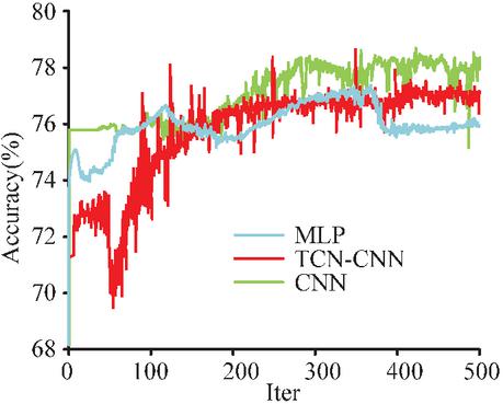
Figure 10 Accuracy of transfer training for different AD models (evaluating the generalization ability of the model on unfamiliar datasets and revealing the issue of decreased accuracy of static models in transfer scenarios).
According to Figure 10, the three models did not perform as expected on another dataset, with accuracy ranging from 70% to 80%. In contrast, the accuracy was not improved, but was rather lower. A model trained on one dataset cannot be directly used for AD in another dataset. For this purpose, the experiment randomly selected 3 sets of 10 batches of data from another dataset for transfer training of the three models, and the results are shown in Figure 11.
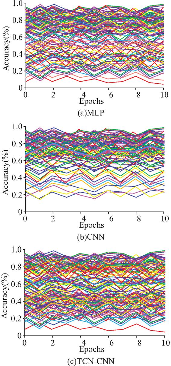
Figure 11 The number of iterations required for the model to achieve different accuracies in the transfer training (quantifying the number of iterations required for the model to achieve a specific accuracy in transfer training, and verifying the model’s ability to quickly adapt to unfamiliar data).
According to Figure 11, CNN has stronger adaptability to unfamiliar data and improves overall accuracy faster. When its accuracy reaches 95%, the average number of iterations trained on the three sets of data is 131. However, the adaptability of MLP and TCN-CNN is relatively weak. Experimental data shows that when the accuracy reaches 80%, the average number of iterations for MLP is 58, and the average number for TCN-CNN is 79, which is higher than MLP. When the accuracy reaches 90% and 95%, the average number of iterations for MLP is 141, 327, and the TCN-CNN is 135, 235, which is lower than MLP. The TCN-CNN model has fewer iterations than the MLP model when achieving higher accuracy. The reason for the poor performance of TCN-CNN on another set of data may be due to overfitting on the first dataset, which reduces its adaptability to other datasets. Therefore, the model parameters at the first training accuracy of 88%, 90%, 92%, 94%, 96%, and 98% were retained, and 10 batches of data from another dataset were trained under each model parameter. Figure 12 shows the corresponding iterations.
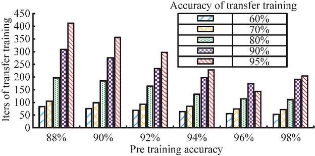
Figure 12 Impact of different pre-training accuracy on transfer training iterations (analyzing the correlation between pre-training accuracy and transferring training efficiency, and determining the optimal pre-training accuracy threshold to balance the risks of overfitting and underfitting).
According to Figure 12, the higher the training level before the model’s pre-training accuracy reaches 96%, the less training time is required for transfer training. When the pre-training accuracy reaches 98%, the iteration of transfer training actually increases. Before the pre-training accuracy reached 96%, this model did not learn enough data features, resulting in the additional iterations when facing unfamiliar data. After the pre-training accuracy reaches 96%, the pre-training process learns too many data features, requiring multiple parameter adjustments when facing unfamiliar data, resulting in transfer training iteration increasing. Therefore, in the subsequent simulation experiments of the adaptive detection system, parameters with a pre-training accuracy of 96% were used. The migration training module can temporarily store 20 batches of virtual machine monitoring data, with each batch set to 10 iterations. To further verify the robustness and generalization ability of the above-mentioned pre-training accuracy threshold (96%), rather than being specific to the initial experimental dataset, a cross-dataset sensitivity analysis was conducted in the study. We selected the financial cloud dataset (for high-frequency trading scenarios), the medical cloud dataset (for scenarios with high IO stability requirements), and the mixed-load dataset described in Section 4.1 and conducted transfer training experiments under model parameters with pre-training accuracy rates of 92%, 94%, 96%, and 98%, respectively. The experiment recorded the average number of iterations required for each model to achieve a 95% detection accuracy rate on different target datasets. The results are shown in Table 6.
Table 6 Analysis of transfer training efficiency with different pre-training accuracy thresholds on multiple datasets
| Pre-training accuracy threshold | 0.92 | 0.94 | 0.96 | 0.98 |
| Financial cloud dataset (number of iterations) | 158 | 132 | 121 | 140 |
| Medical cloud dataset (number of iterations) | 145 | 128 | 118 | 135 |
| Mixed-load dataset (number of iterations) | 168 | 142 | 125 | 152 |
| Average number of iterations | 157 | 134 | 121.3 | 142.3 |
When the pre-training accuracy threshold is 96%, the model demonstrates the highest migration efficiency (with the lowest average number of iterations at 121.3) on all three heterogeneous datasets and performs most stably on each dataset (with the least fluctuation in the number of iterations). This confirms that 96%, as a balance point, can effectively coordinate “feature learning sufficiency” and “model generalization” under multiple data distributions. When the threshold is lower than 96% (92%, 94%), the model does not fully learn the general features of the source domain, resulting in the need for more iterations during migration to adapt to the new data. When the threshold is too high (98%), the model may overfit the source data, and its specialized features hinder rapid adaptation to new fields, resulting in a decline in migration efficiency. This “inverted U-shaped” rule remains consistent in all three datasets. Therefore, the 96% pre-training accuracy threshold demonstrates excellent cross-dataset robustness in the cloud monitoring metric anomaly detection task defined in this study and can serve as an effective empirical configuration reference.
4.3 Simulation Experiment Analysis of an IaaS Cloud Adaptive AD System Combining DQN and CNN
The experimental environment still utilizes a typical IaaS cloud for teaching and research laboratories. For the simulation experiments, data from the experiment is used, and the data is loaded in the following order: training data used by the model, a randomly mixed dataset consisting of training data already used by the model and another set of unused data, and another set of unused data by the model. The experiment is directly carried out on a target virtual machine. The experiment actively generates anomalies through fault injection, analyzes the experimental results and monitoring data, and obtains the abnormal detection accuracy of the detection model on the virtual machine. The decision process of the DQN model is analyzed before testing the simulation performance of the adaptive anomaly detection system. The model was simulated using the pre-training dataset and another dataset and after one round of training; the results are shown in Figure 13.
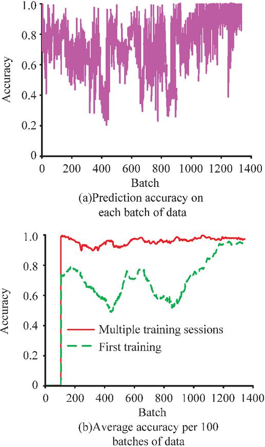
Figure 13 Change in accuracy of DQN model training (displaying the dynamic changes in batch accuracy and average accuracy during model training and verifying the improvement effect of experience replay mechanism on learning stability).
Figure 13(a) shows the prediction accuracy of the model on each batch of data, while Figure 13(b) shows the average accuracy of each 100 batches of data. Analysis shows that the average accuracy of this system in early stages is 0, indicating that the DQN needs to observe and store enough data before starting learning. This study began training after the DQN experience pool data exceeded 300 batches. Therefore, after a round of training, the DQN began to adjust AD. Compared to the previous section, the training results in the latter section are better and the adjustment range is greater because the latter simulation process trained the valuation network of the DQN. The red curve in Figure 13(b) shows the system output accuracy after multiple training and adaptive adjustment of AD by the DQN. It indicates that through DQN decision-making, AD accuracy can be stabilized at a high level and its adaptability to unfamiliar data is enhanced. The change result data of the training accuracy rate of the DQN model all have significant statistical significance. Figure 14 shows the comparative results of the output actions of the DQN model.
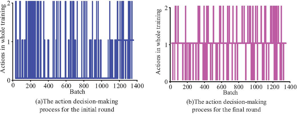
Figure 14 Output results of the DQN model (comparing the distribution of action selection between the initial and final training stages and illustrating the evolution process of DQN strategy from random exploration to stable decision-making).
Figures 14(a) and 14(b) show the comparison of the output action results of the initial and the final rounds, respectively. 0, 1 and 2 represent the constant retention parameters: save the current small batch data and update the anomaly detection model, and reset the anomaly detection model according to the pre-training parameters. The analysis shows that in the initial rounds, the distribution of DQN action decisions is more uniform, and more values are 0. In the final round, the median action decision of 1 is much more than in the other two cases, followed by a value of 0, and finally by a value of 2. It can be seen that the DQN is more inclined to fine-tune the abnormal detection module through small batch data so as to obtain higher detection accuracy. In order to test the practical application effect of the IaaS cloud adaptive anomaly detection system, it was used in the virtual machine for a simulation test and the results are shown in Figure 15.
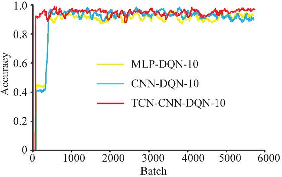
Figure 15 Simulation results of the IaaS cloud adaptive AD system based on the TCN-CNN-DQN model (the detection accuracy and stability of the TCN-CNN-DQN system were comprehensively evaluated and the adaptability of the adaptive decision-making module to dynamic environments was verified).
According to Figure 15, the accuracy of the three models is significantly improved compared to the results without introducing the DQN. Among the three models, TCN-CNN-DQN has the best application effect, with a smaller fluctuation in accuracy compared to the other two models, and the highest accuracy value, ultimately reaching 98%. The simulation result data all have significant statistical significance. Compared with MLP-DQN and CNN-DQN, there is no lower platform period for accuracy in the early training stage, indicating that the model has strong learning and decision-making abilities and stronger adaptability to unfamiliar data. In summary, the TCN-CNN-DQN system has achieved good application results in IaaS cloud adaptive AD. It can effectively improve the detection accuracy of virtual machine anomalies when the user’s operating habits, software installation, and other states are unknown. In order to further analyze the superiority of the research method, a multi-index comparison of the supplementary anomaly detection model was studied, as shown in Table 7.
Table 7 Multi-index comparison of anomaly detection models
| Model | Accuracy (%) | F1 score (%) | ROC-AUC |
| TCN-CNN | 99.8 | 98.7 | 0.997 |
| RNN | 97.8 | 93.2 | 0.941 |
| CNN | 96.5 | 95.1 | 0.963 |
| MLP | 92.3 | 89.5 | 0.892 |
As can be seen from Table 7, in the multi-index comparison of the anomaly detection model the F1 score of the TCN-CNN model is 98.7%, and the receiver operating characteristic area under the curve (ROC-AUC) value is 0.997. It is significantly superior to RNN (F1: 93.2%, AUC: 0.941), CNN (F1: 95.1%, AUC: 0.963), and MLP (F1: 89.5%, AUC: 0.892). The high value of the F1 score indicates that the model can still balance the precision and recall rates in scenarios where abnormal samples are scarce, while a ROC-AUC value close to 1 verifies the model’s strong discrimination ability for positive and negative samples. The performance of research methods with dynamic and adaptive models were compared and analyzed, as shown in Table 8.
Table 8 Multi-index comparison of dynamic/adaptive anomaly detection models
| Average | 12-hour | Concept | ||||
| Detection | False | Drift | ||||
| Accuracy | F1 Score | Latency | Alarm | Robustness | ||
| Model | (%) | (%) | ROC-AUC | (ms) | Rate (%) | Index |
| TCN-CNN-DQN | 98 | 97.6 | 0.995 | 42.3 | 1.2 | 0.91 |
| Autoencoder-based adaptive model | 89.5 | 87.2 | 0.921 | 58.6 | 3.8 | 0.76 |
| LSTM dynamic adjustment model | 93.2 | 91.5 | 0.947 | 65.8 | 2.5 | 0.82 |
| Hybrid LSTM-CNN model | 95.7 | 94.3 | 0.968 | 51.2 | 2.1 | 0.85 |
The concept drift robustness index is calculated based on the average accuracy decay rate in scenarios with 10%/20%/30% feature distribution changes, with a range of values [0,1]. The higher the value, the stronger the robustness. As shown in Table 8, compared with existing dynamic/adaptive models, the TCN-CNN-DQN system still maintains advantages in accuracy, F1 score, and ROC-AUC indicators, especially in low false alarm rate and concept drift robustness. Its detection delay is reduced by about 35% compared to LSTM models, mainly due to the parallel computing architecture of TCN and the lightweight decision-making mechanism of DQN. In the 12 hour continuous operation test, the false alarm rate of the system was always controlled within 1.5%, while the false alarm rate of the model based on autoencoder increased linearly with the running time, indicating that the dynamic parameter adjustment ability of DQN effectively suppressed the performance degradation of the model.
In the hardware environment described in Table 3, TCN-CNN pre-training for 500 rounds took 8.7 hours (with an average GPU utilization rate of 78% and a peak memory usage of 12.3 GB); the DQN controller takes 1.2 hours to train for 10,000 steps (with an average CPU utilization rate of 65%). Compared to static models with the same accuracy, the total training energy consumption is reduced by 28.6%. When monitoring a single virtual machine in real-time, the CPU usage remains stable at 8–12% (single core), with a memory usage of approximately 450 MB. When monitoring 100 virtual machines simultaneously, the peak CPU load on edge servers is 65%, and network transmission overhead is reduced by 42% compared to centralized detection. This indicates that the research method has good computational and energy consumption performance. In the simulation test of the financial transaction cloud environment (processing 8000 virtual machine indicator data per second), the average response delay of the system was 42.3 ms, and the 99.9% percentile delay was 68 ms. When the number of virtual machines was expanded from 100 to 500, the delay increase was only 18%, indicating that the architecture has horizontal scalability.
To verify cross environment generalization ability, three sets of heterogeneous datasets were added for cross validation. The financial cloud dataset contains 1.2 million records (with anomalies accounting for 3.2%, including CPU anomalies caused by high-frequency transactions), the medical cloud dataset contains 800,000 records (with anomalies accounting for 1.8%, mainly due to disk read and write anomalies), and the mixed load dataset integrates e-commerce traffic fluctuations and education cloud memory leakage data (with anomalies accounting for 5.7%). The results showed that the TCN-CNN-DQN model had an average accuracy of 97.2 1.3% and an F1 score of 96.5 1.8% on the three datasets, significantly higher than the static model (accuracy of 89.6 4.2% and F1 score of 87.3 3.5%). It still maintained an accuracy of 95.8% in low anomaly scenarios of medical cloud, reflecting its adaptability to different data distributions. The ablation experiment showed that removing the TCN module reduced the accuracy of the financial cloud dataset by 8.7%, highlighting its role in capturing temporal patterns; removing the CNN module resulted in a 12.3% decrease in the detection rate of abnormal collaboration between medical cloud hard disk and memory; after removing DQN, the accuracy of the mixed dataset decreased by 15.6% within 30 minutes when encountering concept drift, verifying the necessity of dynamic adjustment. The ablation studies demonstrate that the collaborative support of the TCN, CNN, and DQN modules is crucial for maintaining robust and stable detection performance across complex, heterogeneous environments.
5 Conclusion
With the development of CC, there is a massive amount of application and user data stored in cloud systems. If anomalies cannot be detected in a timely manner, it can easily pose hidden dangers to the operational security and stability of the system. Taking the IaaS cloud system as an example, there are four common anomalies that can occur: memory, network, central processing unit, and hard disk. In response to this issue, this study proposes an adaptive AD system based on DQN control. The system is divided into three modules: AD, transfer training, and adaptive control. For AD, a combination of TCN and CNN is used to extract and classify the temporal and spatial features of the data. Then, the migration training module is used to improve the problem of decreased detection accuracy of AD when facing unfamiliar data. Finally, in the adaptive control section, the DQN is used to adjust the model parameters to achieve intelligent control of the system. AD was trained using abnormal data produced by a fault generator. Its accuracy rate is 99.8%, which is better than the single CNN and multilayer perceptron training results, and is 2% more accurate than Google’s Google Net. This indicates that the model has good performance in detecting abnormal data in virtual machines. Transfer training was conducted on the model through three sets of unfamiliar data, and the detection accuracy of the model was less than 80% after 500 iterations. Compared with the trained dataset, its accuracy is significantly reduced. This indicates that if AD cannot adaptively adjust parameters when facing unfamiliar environments, it will reduce the detection accuracy. Following the training of the TCN-CNN-DQN-based IaaS cloud adaptive AD system, its performance was evaluated on a new dataset. It can improve the detection accuracy to over 90% when there is less data and as the data volume increases its accuracy can stabilize at around 98%. Studies show that the TCN-CNN-DQN framework, which integrates spatio-temporal feature extraction and reinforcement learning dynamic decision-making, can effectively solve the static limitations of anomaly detection models in the cloud environment and significantly improve the generalization ability in unknown scenarios. This achievement provides a new paradigm of intelligent operation and maintenance with both high precision and strong adaptability for the field of cloud computing security and promotes the development of dynamic anomaly detection technology based on deep reinforcement learning. The practical application of the system can cover enterprise-level IaaS platforms, virtualized data centers and other scenarios. By monitoring the core indicators of virtual machines in real time and dynamically adjusting the detection strategy, the system can reduce the risk of business interruption caused by resource anomalies and improve the reliability of cloud services. It is thus suitable for industries with stringent stability requirements, such as finance and healthcare. Moreover, several other limitations should be noted. Firstly, although the DQN controller demonstrates strong adaptability in dynamic environments, its responsiveness to abrupt concept drift or highly imbalanced data distributions remains a challenge. In scenarios with extreme class imbalance or rapid workload shifts, the agent may require additional interaction data to stabilize performance, leading to a temporary decline in detection accuracy. Secondly, while the system exhibits good scalability in edge-server deployments, its performance in ultra-large-scale cloud clusters remains to be validated. Additionally, the current model lacks explainability mechanisms, which may hinder troubleshooting and trust in operational practices. The DQN agent relies solely on VM-level metrics without incorporating higher-level contextual information such as user behavior patterns or workload semantics, which could further enhance decision-making robustness. For future work, several directions are recommended. Firstly, integrating explainable AI modules could improve model interpretability and facilitate root cause analysis of anomalies. Secondly, deploying the system in live cloud environments for long-term validation would strengthen the practicality of the approach. Furthermore, extending the state space of the DQN to include user behavior features and workload context could significantly improve the adaptability and accuracy of anomaly detection. Finally, future work will prioritize exploring integrated explainable artificial intelligence methods, such as introducing an attention mechanism to the DQN policy network, to visually reveal its decision-making basis, such as which changes in performance indicators trigger parameter adjustments, thereby enhancing the trust of operation and maintenance personnel in the system. Also, assist in conducting root cause analysis of faults. To address the system’s response challenges to concept drift and severely class-imbalanced data, future research will introduce adaptive learning mechanisms, such as using dynamic experience playback buffers and online fine-tuning strategies to accelerate adaptation to new distributions. Meanwhile, focal loss or adaptive category weights are integrated into the loss function of the detection model to more systematically alleviate the bias caused by the scarcity of abnormal samples, thereby enhancing the continuous learning ability and robustness of the model in the dynamic cloud environment.
Declarations
Fundings
This paper is no funding.
Data Availability Statement
The data are within the text.
Conflict of Interest Statement
There is no conflicts of interest.
Author Contributions
Li Chen, contributed to the motivation, the interpretation of the methods, and wrote the article; Jia Xu, provided the revised article, the data analysis and results, references; Fan Gou provided the data and results, the revised article. All authors approved the manuscript.
References
[1] C. Gan, Q. Feng, X. Zhang, Z. Zhang, and Q. Zhu, “Dynamical propagation model of malware for cloud computing security,” IEEE Access, vol. 8, no. 1, pp. 20325-20333, Jan. 2020.
[2] H. Xu, G. Pang, Y. Wang, and Y. Wang, “Deep isolation forest for anomaly detection,” IEEE Trans. Knowl. Data Eng., vol. 35, no. 12, pp. 12591–12604, Apr. 2023.
[3] R. Ranjbarzadeh, N. Tataei Sarshar, S. Jafarzadeh Ghoushchi, M. Saleh Esfahani, M. Parhizkar, Y. Pourasad, et al., “MRFE-CNN: Multi-route feature extraction model for breast tumor segmentation in Mammograms using a convolutional neural network,” Ann. Oper. Res., vol. 328, no. 1, pp. 1021–1042, May 2023.
[4] Y. Baghoussi, C. Soares, and J. Mendes-Moreira, “Corrector LSTM: Built-in training data correction for improved time-series forecasting,” Neural Comput. Appl., vol. 36, no. 26, pp. 16213–16231, May 2024.
[5] Z. Li, L. Tian, Q. Jiang, and X. Yan, “Fault diagnostic method based on deep learning and multimodel feature fusion for complex industrial processes,” Ind. Eng. Chem. Res., vol. 59, no. 40, pp. 18061–18069, Oct. 2020.
[6] J. Liu, J. Bai, H. Li, and B. Sun, “Improved LSTM-based abnormal stream data detection and correction system for internet of things,” IEEE Trans. Ind. Inform., vol. 18, no. 2, pp. 1282–1290, Feb. 2022.
[7] J. Hu, X. Zhang, and S. Maybank, “Abnormal driving detection with normalized driving behavior data: A deep learning approach,” IEEE Trans. Veh. Technol., vol. 69, no. 7, pp. 6943–6951, May 2020.
[8] M. Raichura, N. Chothani, and D. Patel, “Efficient CNN-XGboost technique for classification of power transformer internal faults against various abnormal conditions,” IET Generation, Transm. & Distrib., vol. 15, no. 5, pp. 972–985, Mar. 2021.
[9] Y. Xin, J. Wang, and H. Wei, “Hybrid fuzzy integrated convolutional neural network (HFICNN) for similarity feature recognition problem in abnormal netflow detection,” Neurocomputing, vol. 415, no. 1, pp. 332–346, Jul. 2020.
[10] Y. T. Quek, W. A. Tso, W. L. Woo, N. T. Koh, and L. L. Koh, “Deep Q-network implementation for simulated autonomous vehicle control,” IET Intel. Transp. Syst., vol. 15, no. 7, pp. 875–885, Jul. 2021.
[11] Y. Zheng, Q. Sun, Z. Chen, M. Sun, J. Tao, and H. Sun, “Deep Q-Network based real-time active disturbance rejection controller parameter tuning for multi-area interconnected power systems,” Neurocomputing, vol. 460, no. 10, pp. 360–373, Oct. 2021.
[12] J. Mei, X. Wang, K. Zheng, G. Boudreau, A. B. Sediq, and H. Abou-Zeid, “Intelligent radio access network slicing for service provisioning in 6G: A hierarchical deep reinforcement learning approach,” IEEE Trans. Commun., vol. 69, no. 9, pp. 6063–6078, Jun. 2021.
[13] Z. Ke, Z. Li, Z. J. Cao, and P. Liu, “Enhancing transferability of deep reinforcement learning-based variable speed limit control using transfer learning,” IEEE Trans. Intel. Transp. Syst., vol. 22, no. 7, pp. 4684–4695, May 2020.
[14] L Bommes, Hoffmann M, Claudia Buerhop-Lutz, T Pickel, J Hauch, C Brabec, A Maier, I Marius Peters. “Anomaly detection in IR images of PV modules using supervised contrastive learning,” Prog. Photovoltaics, vol. 30, no. 6, pp. 597–614, 2022.
[15] S F Kate, H C Marc, Nesar R, L Francois, L Alexie, L Yifei, H Song, P J Xavier, “Anomaly detection in Hyper Suprime-Cam galaxy images with generative adversarial networks,” Mon. Not. R. Astron. Soc., vol. 508, no. 2, pp. 2946–2963, 2021.
[16] B. Mohammed, I. Awan, H. Ugail, and M. Younas, “Failure prediction using machine learning in a virtualised HPC system and application,” Cluster Comput., vol. 22, no. 2, pp. 471–485, Jun. 2019.
[17] F. Cerveira, R. Barbosa, H. Madeira, and F. Araujo, “The effects of soft errors and mitigation strategies for virtualization servers,” IEEE Trans. Cloud Comput., vol. 10, no. 2, pp. 1065–1081, Feb. 2020.
[18] Z. Zhang, J. Wen, J. Zhang, X. Cai, and L. Xie, “A many objective-based feature selection model for anomaly detection in cloud environment,” IEEE Access, vol. 8, no. 3, pp. 60218–60231, Mar. 2020.
[19] S. D. Hallgrímsson, H. H. Niemann, and M. Lind, “Unsupervised isolation of abnormal process variables using sparse autoencoders,” J. Process Control, vol. 99, no. 9, pp. 107–119, Mar. 2021.
[20] M. Razian, M. Fathian, H. Wu, A. Akbari, and R. Buyya, “SAIoT: Scalable anomaly-aware services composition in cloudiot environments,” IEEE Internet Things J., Mar. 2021.
[21] M. Fahim andA. Sillitti, “Anomaly detection, analysis and prediction techniques in IoT environment: A systematic literature review,” IEEE Access, vol. 7, no. 1, pp. 81664–81681, Jan. 2019.
[22] X. Chen, J. Chen, D. Zhao, and X. Jin, “Anomaly detection based on IO sequences in a virtual machine with the markov mode,” J. Tsinghua Univ., vol. 58, no. 4, pp. 395–401, Apr. 2018.
[23] E. Ataie, R. Entezari-Maleki, S. E. Etesami, B. Egger, D. Ardagna, and A. Movaghar, “Power-aware performance analysis of self-adaptive resource management in IaaS clouds,” Future Gener. Comput. Syst., vol. 86, no. 11, pp. 134–144, Mar. 2018.
[24] Y. Hui, “A virtual machine anomaly detection system for cloud computing infrastructure,” J. Supercomput., vol. 74, no. 11, pp. 6126–6134, Nov. 2018.
[25] Z. Chen, “Research on internet security situation awareness prediction technology based on improved RBF neural network algorithm,” J. Comput. Cogn. Eng., vol. 1, no. 3, pp. 103–108, Mar. 2022.
[26] A. Vms and B. Kse, “An improved dynamic fault tolerant management algorithm during VM migration in cloud data center,” Future Gener. Comput. Syst., vol. 98, no. 9, pp. 35–43, Sep. 2019.
[27] A. Zhu, Z. Tang, Z. Wang, Y. Zhou, S. Chen, F. Hu, and Y. Li, “Wi-ATCN: Attentional temporal convolutional network for human action prediction using wifi channel state information,” IEEE J. Sel. Top. Signal Process., vol. 16, no. 4, pp. 804–816, Jun. 2022.
[28] Z. Shen, Y. Zhang, J. Lu, J. Xu, and G. Xiao, “A novel time series forecasting model with deep learning,” Neurocomputing, vol. 396, no. 10, pp. 301–313, Apr. 2019.
[29] J. An, G. Liang, L. Wei, Z. Fu, R. Ping, X. Liu, and L. Tao, “IGAGCN: Information geometry and attention-based spatiotemporal graph convolutional networks for traffic flow prediction,” Neural Networks, vol. 143, no. 722, pp. 355–367, Jun. 2021.
[30] Y. Chen, Y. Kang, Y. Chen, and Z. Wang, “Probabilistic forecasting with temporal convolutional neural network,” Neurocomputing, vol. 399, no. 1, pp. 491–501, Mar. 2020.
[31] Z. Yan, J. Ge, Y. Wu, L. Li, and T. Li, “Automatic virtual network embedding: A deep reinforcement learning approach with graph convolutional networks,” IEEE J. Sel. Are. Commun., vol. 38, no. 6, pp. 1040–1057, Apr. 2020.
[32] T. Zhang, K. Zhu, and J. Wang, “Energy-efficient mode selection and resource allocation for D2D-enabled heterogeneous networks: A deep reinforcement learning approach,” IEEE Trans. Wirel. Commun., vol. 20, no. 2, pp. 1175–1187, Oct. 2020.
[33] S. Liu, G. Tian, Y. Zhang, M. Zhang, and S. Liu, “Active object detection based on a novel deep Q-learning network and long-term learning strategy for service robot,” IEEE Trans. Ind. Electron., vol. 69, no. 6, pp. 5984–5993, Jun. 2021.
Biographies

Li Chen is from Huangshi City, Hubei Province. He obtained a bachelor’s degree in network engineering from Wuhan Textile University in 2010 and a master’s degree in finance from Huazhong University of Science and Technology in 2023. His research interests include information communication, cloud computing, and intelligent engineering. From 2019 to present, he has worked as an engineer at Wuhan Wendao Information Technology Co., Ltd. He has published 6 academic papers, 8 research projects, and 4 soft publications.

Jia Xu is from Wuhan City, Hubei Province. She obtained a bachelor’s degree in computer science and technology from Changjiang University in 2006, with research interests in network security and network engineering. She is Information Security Engineer at Wuhan Wendao Information Technology Co., Ltd. From April 2012 to October 2020, she was Deputy Director of Operations and Maintenance Services at Wuhan Wendao Information Technology Co., Ltd. From October 2020 to June 2022, she was Director of Operations and Maintenance Services at Wuhan Wendao Information Technology Co., Ltd. From June 2022 to August 2023, she was Deputy Manager at Wuhan Wendao Information Technology Co., Ltd. She has published 7 academic papers published, 12 research projects, and 6 soft publications.

Fan Gou was born in Shaanxi Province, CHN in 1994. She received the B.S. degree in Information Management and Information System from Zhengzhou University of Aeronautics, China, in 2016 and the M.S. degree in Information Science from Central China Normal University, China, in 2019. From 2019 to 2025, she was an Employee with Wuhan Wendao Information Technology Co., Ltd., Wuhan, China. She is the author of 4 academic articles. Her research interests include data analysis, data governance, computer software, and computer applications.
Journal of Web Engineering, Vol. 25_4, 497–538
doi: 10.13052/jwe1540-9589.2543
© 2026 River Publishers