A Data Alignment Method for Network Packet Capture Based on DBSCAN

Jiarui Lu and Qinggang Su^*

School of Electronic Information, Shanghai Dianji University; Kaiserslautern Intelligent Manufacturing School, Shanghai Dianji University, Shanghai 201306, China; State Key Laboratory of Acoustics, Institute of Acoustics, Chinese Academy of Sciences, Beijing 100190, China
E-mail: suqg@sdju.edu.cn
*Corresponding Author

Received 15 October 2024; Accepted 28 October 2024

Abstract

This paper investigates the issues of packet alignment and consistency among PLC devices based on industrial network environments, aiming to ensure the integrity and accuracy of packets from sender to receiver. To achieve this goal, we propose an anomaly detection method that combines the DBSCAN clustering algorithm with the 3-sigma principle to identify and handle abnormal packets that may occur during transmission. By comparing the data between the sending and receiving ends, and analyzing based on timestamps and data content, we validate the alignment of packets in the network environment. Experimental results demonstrate that the proposed method effectively detects and corrects packet loss or delay jitter, thereby enhancing the reliability of communication between PLC devices and the consistency of data transmission. The scheme presented in this paper enables quicker and more precise identification of packet loss and delays, adapting well to various network load conditions. Further experimental analysis indicates that this method excels in reducing both false positive and false negative rates, and it exhibits good scalability, making it applicable to data alignment and consistency verification in other industrial automation scenarios. Ultimately, this novel solution provides stability and accuracy for data transmission among devices in a network environment.

Keywords: DBSCAN, data alignment, network quality detection.

1 Introduction

In the context of the development of a new era, computer network technology has become an indispensable and important technological means in people’s daily work and life. Current services delivered on top of the Internet, such as video streaming and video conferencing are increasing the required network capacity [1]. Through network technology, information resources can be collected, integrated, processed, and applied, thereby improving information analysis and mining capabilities, constructing big data environments for various industries, providing convenient and fast intelligent information services, and promoting social transformation and development [2]. A subsequent issue is the existence of a large amount of information exchange in large-scale networks. For instance, in stock trading systems, precise management of thousands of customer transactions is required every second, with exact timestamps for buys and sells; even millisecond variations are critical, and every piece of user interaction information must be error-free.

As technology continues to advance and network applications diversify, the complexity of network infrastructure also grows. This complexity makes monitoring and optimizing network performance increasingly difficult. Network performance encompasses various aspects, such as bandwidth, latency, packet loss rate, and jitter. Convergence time, packet losses, network jitter, and network delay are the parameters that were selected for assessment in order to understand network performance [3]. These performance indicators directly affect user experience.

Time series data analysis algorithms have been gaining significant importance in the research community [4]. In network packet capturing, commonly used algorithms include dynamic time warping (DTW), which aims to find an optimal alignment path that ensures the cumulative distance between two time series is minimized under this alignment [5]. Real-time monitoring and analysis of network performance, along with timely detection and resolution of potential issues, are essential measures for maintaining network stability and optimizing user experience. With the rapid development of the internet and network applications, traditional network performance monitoring methods and tools struggle to meet the demands for real-time responsiveness and accuracy.

In industrial automation and control systems, a commonly used tool is the PLC (programmable logic controller), which is a digital computer specifically designed for these tasks. PLCs are widely used in production line automation, equipment control, and building management. The design goal of PLCs is to replace traditional relay control systems, providing higher reliability and flexibility.

The V90 drive controller, used in conjunction with PLCs, is a high-performance motor control device primarily designed for precise control of servo motors and stepper motors. The V90 drive controller can achieve high precision in position, speed, and torque control, making it widely applicable in automated production lines, industrial robots, and equipment testing.

In modern industrial automation systems, operators can remotely monitor and configure PLCs and V90 controllers over the network, significantly enhancing system maintainability and scalability, and making automation control in manufacturing environments more intelligent and interconnected. Several studies have examined the current state of PLC technology that identify its limitations and propose potential solutions [6]. The quality of network communication is critical for the performance and reliability of PLCs and V90 controllers. These controllers are responsible for controlling and monitoring various devices and processes on the production line, and their effectiveness relies on a stable and efficient network environment.

Additionally, with the sharp increase in data traffic and the number of devices, monitoring performance in modern network environments has become increasingly complex. Because of this, realistic network packet captures are needed that cover all appearing aspects of the network environment [7]. Currently, research aimed at optimizing network performance to meet high-demand applications not only helps improve production efficiency but also reduces downtime and maintenance costs, thereby promoting the development of smart manufacturing.

2 Challenges of Packet Alignment and Strategies for Mitigation

Current monitoring technologies and tools often face performance bottlenecks and data processing challenges when handling real-time data in large-scale and dynamic network environments. Conventional network traffic monitoring systems are becoming inadequate [8] and accurate calculation of network latency is a key research focus in the field of networking. Network latency calculation refers to the time delay of data from the initial point to the destination. Based on the results of network latency calculations, trends in network delay during data transmission can be accurately reflected, serving as a basis for network monitoring and management. Therefore, in the face of these challenges, we need new solutions to enhance network performance and reliability.

2.1 Packet Alignment

Packet alignment is an important research topic because finding the timing of data transmission and reception is crucial for calculating delays. In particular, in high-performance and real-time applications, packet alignment involves ensuring that packets transmitted between different network nodes and devices are correctly aligned in time and order, thus guaranteeing the accuracy of data transmission and the system’s real-time performance. Therefore, in industrial network environments, packet alignment between devices is key to ensuring accurate data transmission and effective processing. It is essential to ensure that packets transmitted between different devices are processed in the predetermined order and timing, as packet alignment significantly enhances overall system performance and reduces data loss and latency.

2.2 The Methods for Solving Packet Alignment Issues. Packet Alignment

To address the packet alignment issues in PLC and V90 control systems within industrial network environments and ensure communication quality, it is necessary to analyze packets and assess network quality. Two primary technical methods are commonly used to achieve packet alignment in computer networks: the network time protocol (NTP) or the precision time protocol (PTP) for clock synchronization, and the establishment of a warm-up time window to exclude erroneous packets [9].

2.3 Applications of Clock Synchronization Technologies

In terms of clock synchronization, substantial research has been conducted both domestically and internationally on time synchronization and distribution technologies. Currently, these technologies are primarily applied to the precise clock synchronization of various subsystems within large physical experimental devices. The NTP (network time protocol) and PTP (precision time protocol) are chosen based on different application scenarios.

In less demanding environments, such as general industrial control and basic data communication between devices, the NTP is a common choice. It synchronizes device time over the internet or local area networks to within milliseconds. The NTP is widely used in network devices due to its strong adaptability and ease of deployment, ensuring relatively consistent time across distributed systems by adjusting device clocks. However, because it relies on network transmission delays and jitter, the synchronization precision of NTP is typically in the tens of milliseconds, which may not meet the requirements for high-precision synchronization.

In contrast, in scenarios that require extremely high precision, especially in industrial network environments where packet timing alignment is crucial – such as in smart manufacturing, industrial automation, and data centers – PTP is commonly used. The PTP protocol is a bidirectional communication protocol based on packet exchanges that enables the accurate synchronization of real-time clocks across distributed systems, typically utilized in Ethernet networks. The PTP protocol defines three types of clocks: ordinary clock (OC), boundary clock (BC), and transparent clock (TC) [10] These clocks form a hierarchical structure for master–slave synchronization, with the highest-level master clock providing the reference time for the entire system. By exchanging PTP event messages, slave clocks can synchronize with the master clock and adjust their own time accordingly. Additionally, accurate timestamps in system and event logs are crucial for auditing and troubleshooting, and NTP ensures that all recorded times remain accurate.

2.4 Setting the Warm-up Time Window

In addressing packet alignment issues, setting a warm-up time window is an effective and practical method. This approach introduces a brief warm-up period before formal packet capture, during which any sent or received packets are ignored, thus avoiding misinterpretation of existing packets as new ones. This strategy helps eliminate errors caused by unstable network conditions during the initial capture phase. Specifically, the warm-up window can be implemented by sending some initialization packets prior to data transmission, effectively filling the link. During formal packet capture, these initial packets are excluded, ensuring that subsequent data collection is more accurate and reliable.

2.5 Determining the Sending Window Size

Additionally, determining an appropriate sending window size is crucial. This can be calculated based on the network’s round-trip time (RTT) and the packet sending frequency. For instance, the sending window size can be set as follows: window size $=$ RTT $\times$ packet sending frequency $+$ safety buffer (e.g., 10% of RTT). In practice, the RTT value can be taken as twice the average latency for increased accuracy, while the sending frequency can be derived from counting the number of packets sent in one second. This method not only enhances the accuracy of packet alignment and reduces errors caused by initial interference but also improves the stability and consistency of data transmission in high-load or complex network environments, providing a solid foundation for subsequent analysis and processing. By appropriately setting the warm-up time window, the system’s performance and reliability can be significantly improved, ensuring smooth industrial communication.

2.6 Imitations of the Methods and Application Considerations

While both NTP and PTP can effectively enhance packet alignment accuracy, they have some limitations. NTP offers lower precision and is susceptible to network delays, making it challenging to meet high-precision synchronization needs. On the other hand, PTP can achieve higher synchronization precision but comes with higher costs and deployment challenges, particularly in wide-area networks where its effectiveness may be less than that of NTP. Although setting a warm-up time window can reduce interference from erroneous data, it relies on accurately determining the warm-up phase; if the duration is too long or too short, it may still affect data accuracy. Therefore, in practical applications, additional adjustments may be necessary based on specific scenario requirements to ensure effective packet alignment and minimize errors.

3 Method

This article employs a method that combines DBSCAN clustering analysis with the 3-sigma algorithm. With the rapid increase in data analysis volume and the growing complexity of high-dimensional data distribution, clustering has become increasingly important in numerous applications, including image analysis, text mining, and anomaly detection. DBSCAN is a powerful tool for clustering analysis and is widely used in density-based clustering algorithms [11]. The two basic parameters of this algorithm are the neighborhood radius and the minimum number of points in the neighborhood. The neighborhood radius indicates the range in which a specific data point searches for similar points, while the minimum number of points in the neighborhood specifies the required number of similar points within the neighborhood radius of that point. The DBSCAN algorithm categorizes data points into core points, boundary points, and noise points.

Based on these definitions, the algorithm’s calculation steps can be summarized as sequentially classifying each point into core points, boundary points, and noise points while marking similar data points. After traversing all points, it produces different cluster labels and identifies outliers, excluding the outliers to provide annotations for which cluster the data belongs to. The central concepts are twofold: directly density-reachable, which states that if point p is within the neighborhood of point q and there are at least a minimum number of points M in q’s neighborhood, then point p is directly density-reachable from point q [12]. There is also the concept of density-reachable: if there exists a series of points p1,…,pm in the data, where each point is directly density-reachable, then p $_{m}$ is density-reachable from p $_{1}$ .

Since the DBSCAN algorithm can be used to label outliers in a dataset and classify them accordingly, it is suitable for scenarios where the latency distribution is relatively concentrated in the same round of data matching, but there are significant latency differences across different rounds [13]. The advantage of this algorithm is that it does not require prior knowledge of the number of clusters, making it convenient for handling situations where the specific nature of the data is unclear. The DBSCAN algorithm classifies closely connected sample points into the same class to form a clustering cluster, ultimately dividing all sample points into different clusters to complete the clustering process.

3.1 Outlier Data Cleaning

To prevent the impact of extreme values in the calculation results caused by network latency, such as a significant increase in latency during a specific time period due to network fluctuations or data loss in certain loops, a data cleansing process is required. Finding the normal values that frequently appear in the data by calculating the lower quartile, upper quartile, and using the interquartile range (IQR) boxplot method with a 1.5 times IQR, or by employing the statistical 3-sigma method to eliminate extreme outliers [14]. Here, we choose the latter approach.

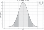
The 3-sigma rule is used to filter the calculated latency results. It is a statistical method used to identify and handle outliers (i.e., extreme values or anomalies). This principle is based on the properties of a normal distribution. As shown in Figure 1, assuming that the data follows a normal distribution, approximately 68% of the data falls within the range of the mean $\pm$ 1 standard deviation. A common way is the 2-sigma or 3-sigma threshold, which theoretically corresponds to a 95% or 99.7% probability, respectively, of falling within the data distribution [15].

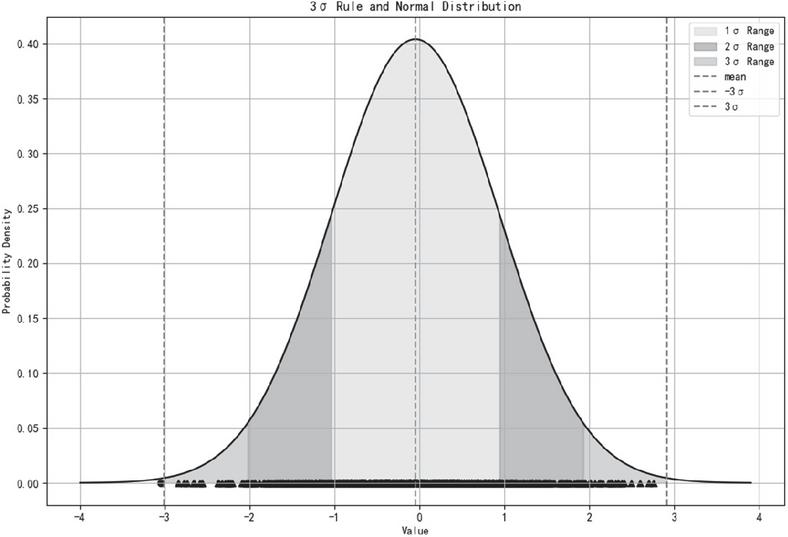
Figure 1 3-Sigma principle diagram.

The 3-sigma rule effectively identifies outliers. In latency data, if a value exceeds the range of $\pm$ 3 standard deviations, this typically only happens to 0.27% of the data. This value can be considered as an anomaly, likely caused by network jitter or interference. By calculating the mean and standard deviation of the data, the normal fluctuation range can be quickly determined, which effectively identifies the normal latency range and aligns the transmission and reception of information accordingly.

3.2 Algorithm Process

Step 1: Mark all sample points in the given data as unvisited, denoted as unvisited.

Step 2: Select any unvisited object P from the data D and mark P as visited.

Step 3: Determine whether P is a core object. A core object is defined as having at least MinPts (where MinPts represents the minimum number of points) within its epsilon-neighborhood. If P is not a core object, mark P as a noise point and then move to the next unvisited object in D. If P is a core object, create a new cluster C for P and add all directly density-reachable points within P’s neighborhood to the candidate set N. Then, proceed to step 4.

Step 4: Access the object point P’ in N. If P’ has already been visited (i.e., marked as visited), it can be added to cluster C. If P’ is unvisited: (1) First, mark P’ as visited. (2) Determine whether P’ satisfies the core point requirement, i.e., whether the number of points in its epsilon-neighborhood is greater than or equal to MinPts. If P’ is a core point, add P $^{'}$ to cluster C and include all directly density-reachable points within the neighborhood of P $^{'}$ to the candidate set N. If P’ is not a core point, classify P’ as a boundary point and add it to cluster C. Execute step 5.

Step 5: Determine whether there are any unvisited points in the candidate set N. If N still contains unvisited points, execute step 4. If all points in N have been visited, execute step 6.

Step 6: Determine whether there are any unvisited points in the data D. If D still contains unvisited points, repeat steps 2 to 6. If all points in D have been visited, output the clustering results.

3.3 Determining Neighborhood Radius

The DBSCAN algorithm requires the input parameters of the data to be detected, the neighborhood radius, and the minimum number of points. The minimum number of neighbors required for each core point can be relatively quickly determined based on information such as data dimension. However, the neighborhood radius is a critical parameter, as it is used to define the neighborhood range of a data point. When the distance between a data point and other data points is less than or equal to the neighborhood radius, these points are considered to be within the same neighborhood.

The neighborhood radius directly affects the identification of core points: if the number of points within a data point’s neighborhood exceeds the specified minimum number of points, that point is marked as a core point. The formation of clusters depends on the neighborhoods of these core points. The size of the neighborhood radius determines the compactness and density of clusters, thereby influencing the final clustering results. A smaller neighborhood radius may result in the formation of multiple smaller clusters, while a larger radius may merge multiple clusters together. Choosing a reasonable neighborhood radius is crucial for achieving effective clustering results.

Distance functions to compact sets play a central role in several areas of computational geometry. This paper adopts the approach of calculating the k-distance and its rate of change to find the “elbow point” to identify the most suitable neighborhood radius. Calculating the distance of each point to its kth nearest neighbor helps capture the local structure of the data. A smaller k-distance indicates that more points are clustered around this point, reflecting higher density. By calculating the rate of change of the k-distance, significant points of density change can be identified. When the rate of change increases suddenly, it often indicates a significant change in density, providing a criterion for distinguishing between core points and noise or sparse regions.

The elbow position usually indicates that at this distance value, the local density of the points satisfies the clustering conditions of DBSCAN. Therefore, using the rate of change calculation can more objectively choose the elbow position, thus determining the most appropriate neighborhood distance. This method allows DBSCAN to effectively identify clustering structures without relying on prior knowledge or subjective judgment. The concept of k-distance is also widely used in classification algorithms [16]. The k-distance algorithm calculates the distance by converting abstract data into data points with multiple dimensions. Each data point’s position in a multi-dimensional space is determined by its feature values. However, when the dimension of feature data is too high or the number of samples in the training set is large, the computational cost will significantly increase, leading to slower output speeds. Additionally, its effectiveness decreases for uneven distributions. However, when applied to the current scenario, which only targets network latency data, this method can achieve good results.

The process of calculating the neighborhood radius, i.e., finding the elbow point of the data, is as follows: For each point in the dataset, calculate the k-distance for each point. The distance can be calculated using the Euclidean distance formula [17].

d (P, Q) = \sqrt{\sum_{i = 1}^{n} {(P_{i} - Q_{i})}^{2}} .

(1)

Let $P$ and $Q$ be the data points used for calculation, and let n be the number of dimensions. After calculating the k-distance for each point, construct a k-distance array by storing all the k-distance values in an array. Next, sort the array in descending order to obtain an ordered array D(k). Finally, compute the rate of change R for the k-distance values, and identify the point R(i) with the maximum value as the elbow point, which determines the desired neighborhood distance.

R_{(i)} = D_{k (i + 1)} - D_{k (i)}

(2)

3.4 Problem Analysis

During packet capturing, the challenges we face are not only about accurately recording data, but also about having a deep understanding of network communication mechanisms. The transmission of packets in a network inherently involves latency, which can arise from various factors such as network congestion, router forwarding delays, or the characteristics of the protocol itself. The complex and often noisy nature of network traffic data necessitates sophisticated analytical ways [18]. When a user presses the capture button, although the system begins recording at that moment, it does not guarantee that all packets can be captured in real time. Packets that have been sent but not yet received may still be traversing the network even after recording has started, eventually reaching the receiver.

This phenomenon is particularly prominent in real-world applications. Suppose a device sends multiple data requests, and due to network delays, some packets start transmitting before the capture tool is activated. During the capture process, the receiver might receive more packets than the actual number sent. Such occurrences not only impact data integrity but also confuse analysts during traffic analysis: which packets are valid, and which are false records caused by capture delay?

To address this issue, analysts need to carefully examine timestamps, packet sequence, and status to distinguish between valid and redundant packets. Such in-depth analysis can help identify potential problems and reveal the true state of network performance. Ultimately, understanding these complex transmission mechanisms allows us to optimize network configurations more effectively, improve data transmission efficiency, and make more precise judgments when encountering similar capture challenges. Only with a comprehensive understanding of the data transmission process can we navigate complex network environments with confidence.

To address this issue, one approach is to identify the actual time of data reception when the capture starts. However, simply determining the time difference between the first and last recorded packets based on their timestamps and then establishing a time range to determine how many packets were sent and received within that time frame can lead to a new problem. If the time range is rigidly defined, any packets outside this time frame will be directly filtered out and ignored. Suppose many packets were lost before the receiver received the first packet due to some reason; in that case, the starting time of the defined time range would already be very late. This way, the actual packet loss scenario would be excluded from the analysis. If the packet loss situation improved when the recording began, the final recorded data might show a low packet loss rate, despite the actual loss rate being much higher.

If we do not confine the time frame and align the packets directly, we face a new issue. The packets are sent cyclically, and during each cycle, the sequence number may go, for example, from 1 to 65,536 before starting over again from 1. Thus, when aligning the packets, two points must be noted: first, the sending time should be earlier than the receiving time. Due to this, the alignment is not a simple matter of matching packets with the exact same data in the table, as the timestamps will definitely differ. This leads to the second problem: aligning only by the sequence number is insufficient. It is also necessary to determine whether the packets are from the same cycle, as a packet from the previous cycle may match a packet received in the current cycle. Therefore, it is necessary to calculate the time difference. If the time difference falls within a certain threshold, it can be determined that they belong to the same cycle. How should this threshold be determined? Different machines and network conditions yield different results. If we rely solely on experience and subjectively set a threshold, it might result in either failing to match packets from the same cycle or matching packets from different cycles because of an overly large time threshold.

In this study, first prepares data by collecting and organizing network traffic data to lay the foundation for subsequent processing and analysis. During feature engineering, key features such as timestamps, source and destination addresses, and sequence numbers are extracted from the network traffic data to establish a suitable feature set, providing strong support for subsequent clustering analysis. Initial alignment is performed on the raw data, and delay data during the initial alignment is recorded. For abnormal delay values in the delay data, the 3-sigma rule is applied in advance to reduce errors. Since this part of the data is only a small portion of the final data alignment process, it will not be computationally intensive. Moreover, with delay being the only feature, it avoids the issue of inaccurate distances in k-distance algorithm calculations due to the involvement of too many dimensions. After obtaining the parameters needed for the DBSCAN algorithm through the k-distance algorithm, the DBSCAN algorithm is used to cluster delay data from different cycles. This results in clusters formed by different delays, and by analyzing the characteristics of these delays, the difference between clusters represents the normal cycle time. By calculating the differences between clusters, the delay standard can be obtained.

4 Experiment

4.1 Experimental Process

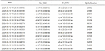
The data used in this experiment comes from the packet capture results recorded during actual testing of the PLC and V90 controller. Before starting the analysis, it is necessary to clarify the format of the captured data and perform a simple classification based on the source and destination addresses to determine the amount of data sent and received at both ends (Figure 2).

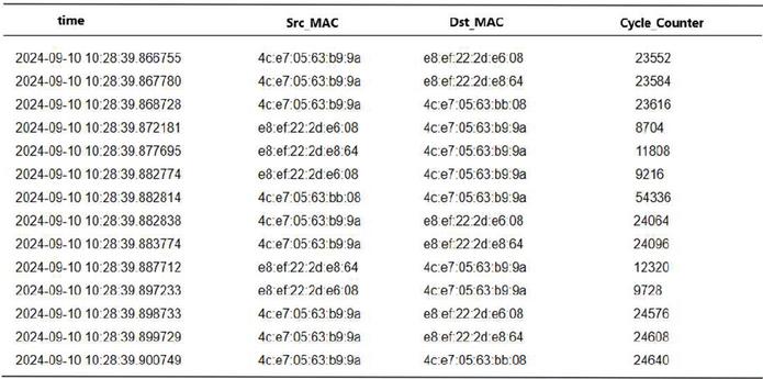
Figure 2 Packet capture data format.

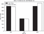
From the analysis of the packet capture data in this experiment, it was observed that two of the three machines experienced packet loss, while the third machine actually received more packets than were sent. Therefore, further data alignment is required based on latency. For Machine 3, a total of 3680 packets were sent by the PLC, while the corresponding V90 controller recorded receiving 4120 packets, with the capture duration being two minutes. Prior to the start of packet capture, a unified server was used for clock synchronization to ensure consistency in time records. After recording the data packets on both the receiving and sending sides, latency standards can be analyzed.

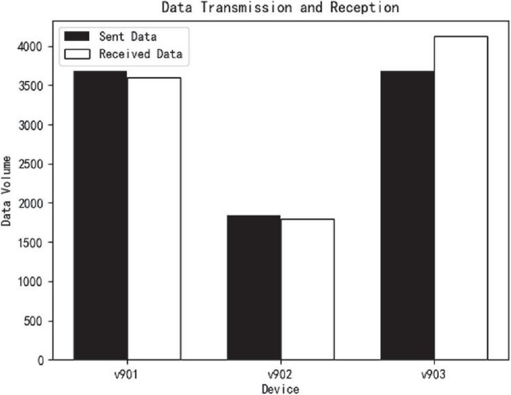
Figure 3 Packet transmission and reception status.

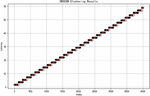
Step 1: For outlier values in the latency data, the 3-sigma principle is applied in advance to clean the data and reduce errors. Then, data with matching values in the cycle counter are paired together as the initial samples. At this stage, no strict matching criteria are enforced; as long as the cycle counter values are the same, the data can be matched. This approach is used to capture the packet latency status between devices in the current network as comprehensively as possible, which helps to analyze the state of the packet cycle count more clearly. A total of 4061 latency data points were matched, and the latency for each pair of data was calculated to create a latency array. The graph of this array (Figure 3) shows an increasing trend, which is due to the characteristics of the cycle counter in the data, where different rounds of data are repeatedly matched.

Step 2: For the latency array obtained in Step 1, the k-distance is calculated using the Euclidean distance.

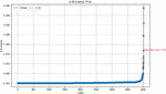
Step 3: All points’ k-distances are sorted in ascending order and a graph is plotted. The y-axis of the graph represents the distance, while the x-axis represents the index of the points. The point with the highest rate of change, known as the elbow, is identified, which corresponds to the domain distance (Figure 4).

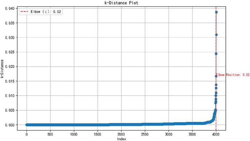
Figure 4 Elbow position diagram.

By observing the k-distance graph, it can be noted that the elbow position is at 0.02. This elbow position indicates where the density of the data changes, and thus, it can also be used as the neighborhood size.

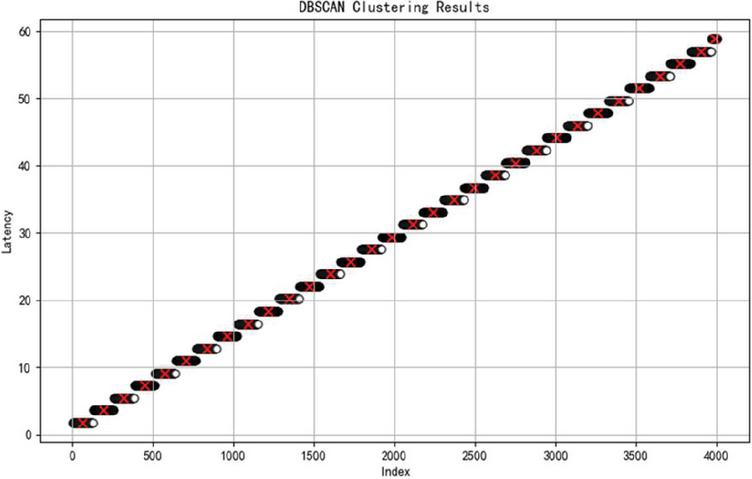
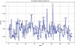
Figure 5 Delay representation after clustering.

Step 4: Using the neighborhood distance obtained in the previous step as a parameter, apply DBSCAN clustering to the latency array to obtain preliminary classification results.

Step 5: Through the DBSCAN clustering analysis (Figure 5), it is observed that the matched data packets from different rounds produce multiple results. This means that when a packet is matched, it may correspond to multiple rounds before or two rounds after, which can lead to analysis errors.

At this point, calculate the differences between the center of each cluster to determine the time for each cycle. The latency difference array at this stage has become very close between each other.

By observing the latency difference array, it can be seen that the latency is mostly around 1.73 (Figure 6). In practical applications, this level of precision is sufficient to distinguish between packets from different cycles. A standard latency of 1.74 is chosen for secondary matching, resulting in 3660 matched packets. Compared to the previous 3680 sent packets and 4120 received packets, this more accurately reflects the network’s packet loss rate and latency conditions.

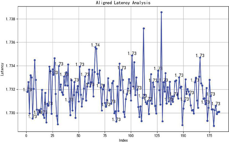
Figure 6 Final confirmed delay variation range.

4.2 Results Analysis

Although the data packets contain timestamps and loop counters for correspondence, due to the possibility of packet loss, even if the number of recorded packets on both the sending and receiving sides is known, the difference cannot be directly used to determine the number of abnormal records. If alignment is based solely on whether the loop counters are the same, the result will disregard the existence of loops, causing latency values to range from a minimum to negative numbers, or even accumulate over several loop times. This clearly contradicts the concept of one-to-one packet matching analysis. Since a packet can only be matched once in the matching algorithm, an incorrect packet alignment may result in multiple incorrect matches, ultimately leading to significant errors in overall calculations.

Even with the introduction of a preheating window, which can reduce latency to some extent and eliminate some misaligned packets, it still cannot completely and efficiently handle packet alignment. Therefore, in this scenario, we use a method that combines the density-based DBSCAN algorithm with the 3-sigma principle to establish a standard of normal latency for packets, thereby achieving packet alignment. Since DBSCAN is a density-based clustering algorithm, when calculating the latency of packet sending and receiving, situations often arise where packets match with those from the previous round, the next round, or even further rounds. Therefore, when calculating latency, data matched from different rounds can be grouped into different clusters. By calculating the difference between clusters of different rounds, it is possible to dynamically obtain the latency of packets at different times.

Moreover, to address packet latency anomalies caused by network errors and to more accurately determine the latency standard, the 3-sigma principle is introduced to clean latency values affected by network anomalies in the latency array, reducing the impact of extreme values. In this experiment, it was found that the time difference between Device No.1 (PLC) and V90 drive controllers No. 1 and No. 2 is mostly around 1.7 seconds, while the time difference with the third drive controller and the other PLC appears to be 5 seconds. Without understanding the configuration between devices, it is impossible to determine an accurate latency standard for different network environments solely based on experience or simple testing. By using the method proposed in this paper – calculating the latency standard based on density clustering and inter-cluster differences – the communication quality between different devices in various industrial network environments can be effectively assessed.

5 Conclusion

This paper conducted an in-depth study on packet alignment and consistency issues between PLC devices and proposed an anomaly detection method that combines the DBSCAN clustering algorithm with the 3-sigma rule. With the continuous advancement of industrial automation, the requirements for the reliability and accuracy of data transmission have become increasingly stringent. This research aims to address potential issues such as packet loss and latency jitter in high-speed network environments, ensuring the integrity of information transmitted from the sender to the receiver.

What we need is a method that can dynamically solve problems while minimizing overhead. Some existing methods, such as adding extra information to data before transmission, can improve certain issues, but they are often not lightweight and increase the complexity and overhead of data transmission [19].

One advantage of this method over setting a warm-up time window is that the flexibility in adjusting the window size is limited in many traditional approaches, which may not effectively accommodate varying network conditions. In contrast, this method can adapt more dynamically to fluctuations in network performance. Modern daily life depends on precise time synchronization [20]. Compared to using the precision time protocol (PTP), this method offers a significant advantage in terms of overhead, as the PTP incurs substantial costs in terms of network bandwidth and processing power, making it less efficient in high-performance environments where resource optimization is critical.

Through systematic experimental analysis, the proposed method has been validated for its effectiveness and adaptability under different network load conditions. The results show that the method not only effectively identifies and corrects abnormal packets in a timely manner, but also significantly reduces the false detection and missed detection rates, thereby improving the stability of communication. This provides reliable data transmission assurance for the industrial field, particularly in real-time monitoring and control applications, and holds significant practical value.

Future research can be expanded in the following areas: (1) Further optimizing the algorithm to maintain efficiency in more complex network environments; (2) exploring integration with other advanced technologies, such as machine learning and edge computing, to enhance the system’s intelligence; and (3) conducting field tests in various industry applications to verify the method’s versatility and scalability.

In conclusion, this study provides an innovative solution for industrial communication in industrial network environments. It not only lays a solid foundation for data alignment and consistency verification, but also opens up new directions for future research in related fields. It is hoped that this study will contribute to the advancement of industrial automation technology and the improvement of data transmission security.

Declaration of Competing Interest

The authors declare that they have no known competing financial interests or personal relationships that could have appeared to influence the work reported in this paper.

Acknowledgments

Supported by the State Key Laboratory of Acoustics, Chinese Academy of Sciences (grant No. SKLA202411).

References

[1] Adanza D, Gifre L, Alemany P, et al. Enabling traffic forecasting with cloud-native SDN controller in transport networks[J]. Computer Networks, 250110565–110565, 2024.

[2] Qiongqiong S, Longfei Y. Enhanced computer network security assessment through employing an integrated LogTODIM-TOPSIS technique under interval neutrosophic sets[J]. International Journal of Knowledge-based and Intelligent Engineering Systems, 28(3):419-434, 2024.

[3] Shahid K, Ahmad N S, Rizvi H T S. Optimizing Network Performance: A Comparative Analysis of EIGRP, OSPF, and BGP in IPv6-Based Load-Sharing and Link-Failover Systems[J]. Future Internet, 16(9): 339–339, 2024.

[4] Luo Y, Ke W, Lam T C, et al. An accurate slicing method for dynamic time warping algorithm and the segment-level early abandoning optimization[J]. Knowledge-Based Systems, 300112231–112231, 2024.

[5] Gao Wei, Qian Chengyang, Zhang Qi, et al. Trajectory similarity algorithm based on dynamic time warping and trajectory point compression [J/OL]. Control and Information Technology, 1–8, 2024.

[6] Beqirllari K, Ozansoy C, Gomes D, et al. High-bandwidth coupling circuit design for PLC applications on SWER networks: From design to production[J]. Engineering Science and Technology, an International Journal, 58101840–101840, 2024.

[7] Daniel S, Jörg K. Requirements for Crafting Virtual Network Packet Captures[J]. Journal of Cybersecurity and Privacy, 2(3):516–526, 2022.

[8] Zhongxing D. Network Traffic Monitoring Algorithm Based on Big Data Analysis[J]. Academic Journal of Computing & Information Science, 6(5), 2023.

[9] Yang Xuerong, Wang Longfei, Yuan Ranhui, Shan Shangqiu. Cooperative Objective-Oriented Multi-UAV Clock Synchronization Algorithm [J]. 32(6): 573–578, 2024.

[10] Cheng Shunling, Li Changxian, Zhao Ke. Optimization of Train Communication Network Time Synchronization Based on PTP Protocol [J]. 45(18): 92–98, 2022

[11] Cai Z, Gu Z, He K. A self-adaptive density-based clustering algorithm for varying densities datasets with strong disturbance factor[J]. Data & Knowledge Engineering, 153102345–102345, 2024.

[12] Zhang Yanlong, Zhu Huabing, Liu Zhengyu, Wen Jian. Depth Grouping Method for Retired Power Batteries Based on DBSCAN Clustering [J]. Power Technology, 47(4): 462–468, 2023.

[13] Ge Chengpeng, Zhao Dong, Wang Rui, Ma Qinghua. Segmented Point Cloud Denoising Method Based on Improved DBSCAN and Distance Consensus Evaluation [J]. Journal of System Simulation, 1–11, 2024.

[14] Liao Yong, Huang Lei. Research on the Design of Operation and Maintenance Platform and Anomaly Detection Based on Microservices, 2021.

[15] Hermans C, Koussa A J, Oevelen V T, et al. Fault detection for district heating substations: Beyond three-sigma approaches[J]. Smart Energy, 16100159–100159, 2024.

[16] Ding Zuokun, Ding Jingjing. Optimization of Human Settlement Environment Improvement Based on Information Technology [J]. Modern Computer, (08): 54–59, 2021.

[17] Shi Linjun, Dai Tao, Lao Wenjie, Wu Feng, Lin Keming, Li Yang, Zhu Ling, Huang Xifang. Operational State Recognition of New Energy Power Generation Units Based on Improved KNN Algorithm, Power Automation Equipment.

[18] Olabanjo O, Wusu A, Aigbokhan E, et al. A novel graph convolutional networks model for an intelligent network traffic analysis and classification[J]. International Journal of Information Technology, (prepublish):1–13, 2024.

[19] Abdulabbas FAA Barbaros P. Effect of Sliding Windows Technique on the Performance of TCP/IP Networks[J]. Journal of Smart Internet of Things, 1(1):46–55, 2023.

[20] Kumar K, Ghosh K S, Neelam, et al. Indian Standard Time Dissemination Using Precision Time Protocol: Toward Resilient Time Synchronization Using Optical Fibers for Critical Infrastructure in India[J]. MAPAN, 39(3):475–482, 2024.

Biographies

Jiarui Lu is currently a master’s student in the School of Electronic Information at Shanghai Dianji University, having enrolled in 2023. His research focuses on industrial big data processing and analysis.

Qinggang Su received his B.Sc. degree in Computer Science from Anhui University of Technology in 2002, obtained his M.Sc. degree in Communication Engineering at Shanghai Jiao Tong University, and his Ph.D. degree at East China Normal University. He is the vice dean of Aeronautics School, Shanghai Dianji University. He is a member of China Computer Federation (CCF), and his research is currently focused on wireless networks, 5G application, smart manufacturing and industrial big data.