Overcoming Terrain Challenges with Edge Computing Solutions: Optimizing WSN Deployments Over Obstacle Clad-Irregular Terrains
Shekhar Tyagi and Abhishek Srivastava
Department of Computer Science and Engineering, Indian Institute of Technology, Indore, India
E-mail: phd2201101013@iiti.ac.in; asrivastava@iiti.ac.in
*Corresponding Author
Received 30 September 2024; Accepted 09 November 2024
Abstract
Wireless sensor networks (WSNs) are primarily used for real time data collection and monitoring, especially in environments where direct human involvement is challenging due to harsh conditions. Optimized deployment of WSN nodes is a long standing issue and several ideas have been proposed to address this. Existing deployment strategies are mostly based on the assumption that the terrain for deployment of nodes is perfectly regular. This is an impractical assumption and in this paper we address this gap by proposing a deployment strategy for WSN nodes over irregular terrains. Such terrains comprise uneven elevations, morphology and vegetation based obstacles, rocky obstacles, and so on. Our approach comprises extraction of satellite images of the region of interest (RoI) from Google Earth and generating a KML file (Keyhole Markup Language) for the RoI containing the latitude, longitude, and elevation values of each and every point in the RoI. These points are used to generate a contour map of the RoI containing detailed terrain morphology. A radio frequency path loss model in combination with an advanced inverse distance weighted (IDW)-interpolation technique is proposed to ensure connectivity and coverage in such irregular terrains with varying nature of obstacles. The technique effectively detects occlusions and enables effective deployment. This edge computing approach involves real-time decision-making at the network edge (the sensor nodes) leading to a deterministic deployment of motes in diverse terrain conditions with various obstacles. The approach is compared with existing deployment techniques and the results validate its efficacy. To demonstrate the practicality of our approach, we have also implemented a deployment in real-world environmental conditions, validating our approach in challenging terrains.
Keywords: Wireless sensors, irregular-terrain, obstacles, sensor deployment.
1 Introduction
A wireless sensor network (WSN) is a decentralized system composed of tiny devices called motes or sensors that are distributed to form an ad-hoc network over a specified region of interest. The motes monitor and record the values of parameters of interest and communicate the same over ad-hoc networks to back end servers for detailed analysis. A WSN has a variety of applications across domains ranging from environmental monitoring to healthcare [1]. WSNs are ideal for various defence applications such as target tracking operations in stealth mode and monitoring disasters like forest fires, land slides, glacier displacements, and so on.
An important challenge in WSNs is optimal deployment of motes. This is especially so because motes are relatively expensive and the area to be covered is often large. Several strategies have been proposed in the past by researchers for WSN deployment but most of these strategies were largely confined to flat terrains. A few studies have considered three-dimensional regular terrain [9, 11, 12, 14, 15] but a very limited number of studies have focused on irregular terrain [16, 17]. Those that considered irregular terrain often dealt with non-obstructed terrain or included an obstacle without specifying the obstacle type. WSN deployment strategies in the literature include nature inspired heuristic approaches like particle swarm optimization (PSO) [2] which takes inspiration from avian and aquatic social behaviors and proposes deployment strategies along these lines. Kulkarni et al. [3] explore a bio inspired technique for WSN deployment that utilizes PSO with multidimensional optimization parameters to enhance coverage and connectivity in WSN deployment. Deif et al. [4] propose an ant colony optimization approach combined with a local search heuristic algorithm. They suggest a non-overlapping minimally connected coverage strategy for the desired deployment region of interest. You et al. [5] propose a Voronoi polygon based method that divides the region of interest into unique cells based on proximity and optimizes local coverage using angle of view techniques. Tang et al. [6] implement a non-dominating sorted genetic algorithm with Voronoi polygons to obtain the sensing radius and communication radius. Subsequently, they calculate the fitness function with genetic algorithms for optimized deployment. The approach in [7] comprises a Delaunay deterministic deployment method that computes a DT score (Delaunay triangulation score) in which, prior to deployment, every candidate location generated from the current sensor configuration is saved by a probabilistic sensor detection model. A sensor is then placed at a potential location that has the best coverage gain. Yan et al. [8] propose a Steiner-tree based algorithm and consider aspects of algorithmic complexity and real topology to implement improved deployment strategies by selecting proper representative points and recovery strategies to minimize the cost of node deployment.
The major gap in these studies is their predominant focus on flat terrains and regular 3D terrains, leaving irregular terrains with varying obstacle types relatively less explored. Approaches that endeavor to provide solutions for irregular terrains fall short in terms of scaling to large settings. Our proposed approach majorly deals with the complexities of irregular terrains with various obstacles types like vegetation, rocks, etc. This paper further builds upon [18], which proposed an optimized obstacle-aware sensor deployment technique for irregular terrains. In contrast to the workshop paper, this paper includes a comprehensive complexity analysis, deployment time estimation model, a detailed real-world case study within the Melghat Tiger Reserve, and thorough comparative evaluations with state-of-the-art methods. These additions validate the efficiency and applicability of the proposed technique across a diverse range of complex terrains.
The remainder of this paper is organized as follows: Section 2 provides a background on existing approaches; Section 3 discusses the proposed methodology in detail, Section 4 comprises comprehensive experiment description and results that validate the efficacy of the proposed approach through comparisons with existing methods, followed by a real world deployment. Finally, Section 5 concludes the paper.
2 Background Work
This section provides a detailed overview of key methods, highlighting their contributions and limitations in handling WSN deployment challenges over uneven and obstacle-laden terrains. Li [9] was the first to introduce the digital elevation model utilizing the PSO technique for sensor coverage, incorporating both local and global search mechanisms with PSO to optimize coverage over the grid, termed 2.5D. Udgata et al.[10] propose a method of deployment inspired by honeybee foraging in which sensor deployment is modeled as a data clustering problem. The scheme deploys a few motes and compares them with a limited rectangular terrain without taking into consideration elevation and signal attenuation for range estimations. This results in computational scalability issues in optimization over large scale deployments. Fu et al. [11] propose a WSN deployment method over 3D terrains using a probabilistic greedy-coverage algorithm that accounts for signal attenuation, but with a relatively limited communication range of 5 m. The method computes uniform signal attenuation for obstacles and does not consider the varying effects of different obstacle types on signal attenuation.
Bhattacharyya et al.[12] introduce a layered deployment concept with a specialized node defined as a fusion node or a central server. However, this lacks a signal attenuation model and elevation estimations of the fusion node with neighbourhood nodes lead to loss of connectivity. Cheng et al.[13] propose a sensor deployment scheme for a special application for imparting barrier coverage over irregular border areas between two countries to check intruder activities. They utilize a convex hull and turning point selection approach where they segment the area into small n-virtual rectangles. The approach again lacks the capability to scale effectively to larger areas. Du et al.[14] propose a deployment algorithm for a 3D terrain incorporating two heuristic techniques: PSO and virtual force coverage. They propose a communication limit for sensor deployments explicitly, thereby limiting generalizations for signal attenuation and elevation. Combining two heuristic approaches leads issues of scalability here as well. Boualem et al.[15] use a spiderweb technique to deploy motes over a regular 3D surface without obstacles. The method estimates coverage based on the minimum set of deployed motes that remain active after 50 time units. Xiao et al.[16] propose a technique for irregular terrain deployment without considering obstacles. They design a surface coverage method based on grid division and simulated annealing. Liu et al.[17] propose a coverage method for irregular rolling terrains using a vertex triangulation grid based method. While prior studies have enhanced WSN deployment, they lack effective strategies for deployment over irregular terrains. Our approach advances scalability and adaptability by optimizing mote placement, taking into account terrain elevation and signal attenuation to address obstacles effectively.
3 Proposed WSN Deployment Framework for Irregular Terrains
The strategy for WSN deployment, proposed in this paper, is meant for terrains that are irregular in nature and also takes into account obstacles in such terrain like trees, dense grass, and rock formations. The approach comprises: data acquisition by extracting the region of interest from Google Earth; constructing a KML file for the extracted region of interest and generating a contour map offering insights into the topographical complexities of the region; utilizing an inverse distance weighted (IDW) interpolation technique to estimate elevation values at unmeasured points by considering both distance and terrain characteristics; and finally incorporating path loss models in signal communication along with a digital elevation model (DEM)[9] to account for occlusions due to terrain irregularity and obstacles of varying types and making deployments accordingly. We discuss each step of the proposed methodology in the following subsections.
3.1 Extraction of Region of Interest and Terrain Analysis
We begin by acquiring high-resolution satellite imagery and elevation data from Google Earth [19]. Using Google Earth’s tools we select the region of interest (RoI) and save it in a KML format (Keyhole Markup Language format) file. KML is a file format designed for spatial contexts and comprises coordinates and elevations of individual points in the RoI. The KML file is next converted to a GPX (GPS Exchange Data) file using a TCX Converter [20]. A GPX file comprises an XML schema and makes the terrain information contained in the KML file inter-operable. Subsequently, a GPS Visualizer [21] is harnessed to customize and visualize the data in the KML file and generate detailed maps and elevation profiles. The KML file so visualized comprises topographic information through color coding. Light green, for example, indicates sparse vegetation like grass, while dark green signifies dense tree coverage, and so on. These help in obstacle identification while using radio frequency path loss models. An extracted region of interest and a sample CSV file content is shown in Figures 1 and 2.
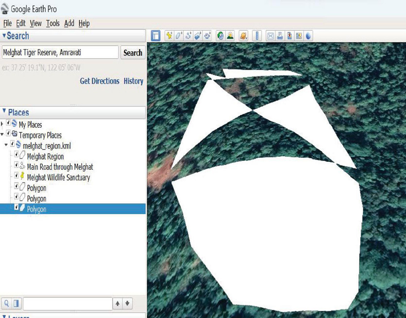
Figure 1 An extracted region of interest.
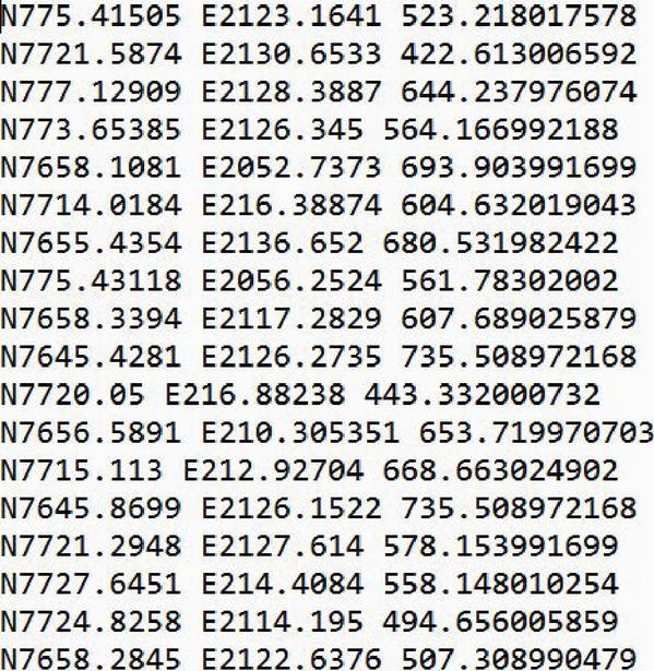
Figure 2 A sample processed KML file content in CSV format for an extracted region of interest.
3.2 Creation of a Contour Map of the Region of Interest
A contour map is a visual depiction of the elevation variations across the landscape and offers valuable insights into the topographical intricacies of the region of interest. This enables more effective deployment of sensor nodes.
Figure 3 shows a three-dimensional surface and the corresponding two-dimensional contour map for the same is shown in Figure 4 [22]. The KML file comprising latitude, longitude, and elevation information is the basis for generating a contour map of the irregular terrain. The KML file, as mentioned earlier, is subsequently transformed into a GPX file that comprises the latitude, longitude, and elevation information of each data point within the region of interest in an inter-operable XML format. The GPX file is processed by a specialized software application called QUICKGRID [22] for contour generation. This process generates the desired contour map of the region, which is used for further processing.
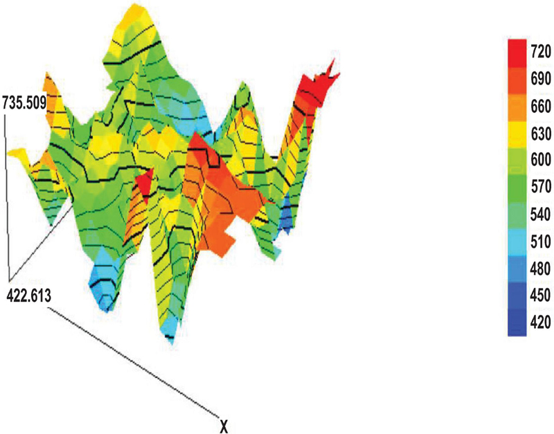
Figure 3 Three-dimensional surface [22].
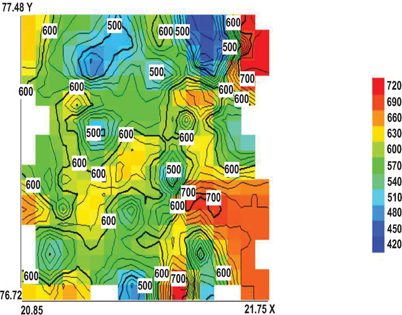
Figure 4 Two-dimensional contour map of the three-dimensional surface [22].
3.3 Path Loss Model for Obstacles
Path loss refers to the attenuation or reduction in signal strength as a radio wave propagates through a medium or travels from a transmitter to a receiver. It may occur owing to factors such as distance, obstacles, and environmental conditions. Integrating path loss models with a contour grid (discussed in the following section) is essential for the deployment of WSN motes as these define the communication range taking into account obstacles of various kinds such as dense natural grass, trees, and rocks. The proposed approach computes the path loss owing to various obstacles and utilises the modified received signal strength indicator (RSSI) for deployment. A comprehensive explanation of the measurement methods and the formation of the models can be found in [23, 24, 25, 26]. The first-order log–distance model is described as follows:
| (1) |
In this equation, represents the benchmark distance or distance field and is typically set to 1 m; is the distance in meters between the transmitting and receiving motes; the median path loss at the reference distance (in dB) is denoted by ; represents the path loss exponent and depicts the loss in signal strength due to the obstacle; and represents the log normal shadowing and compensates for random variations in the signal. The values for the path loss exponent and the shadowing effect values were derived from well-established empirical studies and experiments conducted across various types of obstacles such as trees, grass, and rocks in real-world terrains.
Following this, the path loss model for a terrain with obstacles in the form of trees, grass, and rock formations is as follows:
| (2) |
where the path loss exponent and tree shadowing effect values for trees, grass, and rock are as follows: , , and ; and the shadowing effect values are , , and .
Hence, with known values of effective radiated power (ERP) (the power level at the point of transmission) and received signal strength indicator (RSSI) (the power level at the point of reception), the power loss Pl (dB) in Equation 2 is computed as (ERPRSSI). This enables us to compute the communication range of the motes given the obstacles as follows:
| (3) |
A connection between two or more nodes is established if the Euclidean distance between them is less than or equal to the node range where the Obstacle may be tree, grass, or rock. If the distance exceeds , it implies a signal obstruction or occlusion.
3.4 Creation of a Digital Elevation Map from a Contour Map
A digital elevation map or model (DEM) is a discrete grid-based representation of ground surface topography that transforms the continuous terrain surface representation on a contour map into a series of data points representing longitude, latitude, and elevation. A DEM is created from terrain elevation data and is represented as a grid or raster of the elevation values. Each cell (or pixel) in the raster represents a specific area on the ground, and the value of that cell represents the elevation of that area. A DEM comprises a series of DEM data points of a continuous terrain. Figure 6 shows a simple DEM representation of a corresponding contour plot shown in Figure 5.
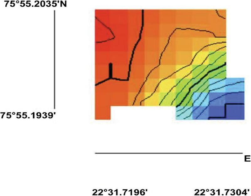
Figure 5 Two-dimensional contour map of a region.
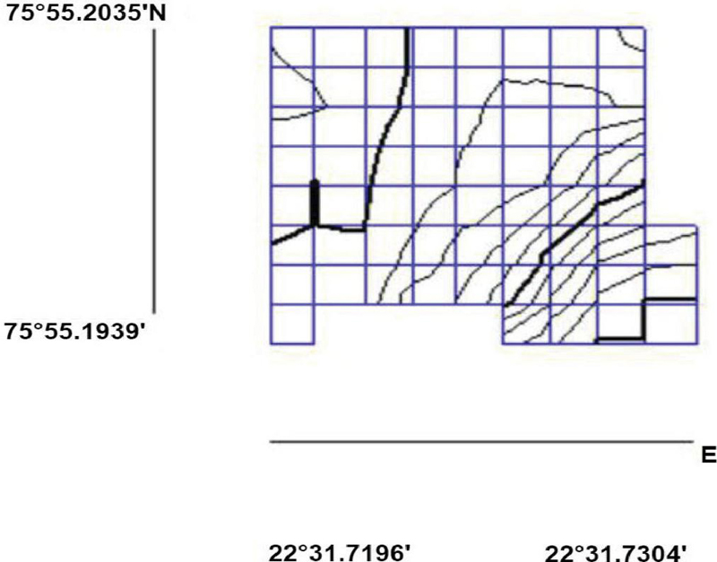
Figure 6 DEM of the corresponding contour plot.
3.5 Elevation Estimation through Inverse Distance Weighted Interpolation
Inverse distance weighted (IDW) interpolation is a robust technique that calculates the value of an unmeasured point based on the weighted average of its neighboring measured points, as shown in Figure 7. A terrain surface is represented in the figure by a DEM grid, depicting a complex landscape. To calculate the elevation of an unmeasured elevation point denoted as P, the process computes its elevation value by utilizing the weighted average values of the measured known elevations of the neighboring points depicted as A, B, C, and D in the figure. A larger distance of a known point from P leads to a smaller weight and hence weaker contribution in computing its elevation and vice-versa. The weights are calculated by the inverse of the distance raised to a power parameter , giving more significance to nearby points in the estimation process. Mathematically, this can be expressed as:
| (4) | |
| (5) |
where is the elevation value of neighboring measured points, is the distance from the deployment point, and is the power parameter.
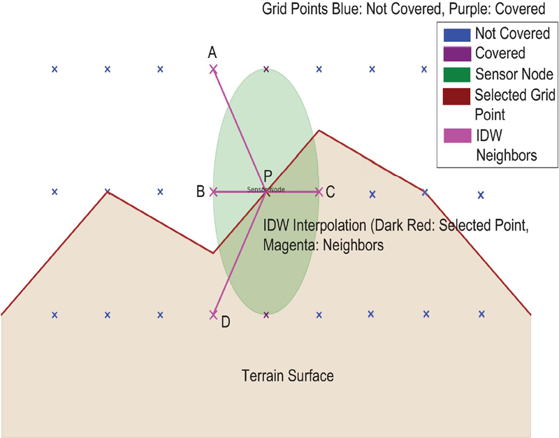
Figure 7 Elevation estimation using IDW interpolation in complex terrains.
3.6 Identification of Potential Mote Deployment Locations
The crux of this work is identification of potential mote deployment points. To do this, a random origin point is chosen in the DEM grid and a perceptual direction, a straight line along the line of sight, is traced from the origin. A potential deployment point on this traced line is chosen and the Euclidean distance and RSSI of the point is computed from the previous node deployment point (this is the origin to start with and changes as the deployment exercise progresses). The Euclidean distance of the point takes into account the coordinates (longitude and latitude information obtained from the extracted information) of the point and its elevation (calculated using the IDW interpolation technique). If the Euclidean distance of this point is larger than the value computed for the respective terrain (trees, grass, or rocky) the point is deemed occluded. Otherwise the point qualifies as a potential deployment point. Subsequent to this, the straight line (denoting the perceptual direction) traced from the origin undergoes angular displacement by and the process is repeated and potential deployment points are identified. This is continued by tracing the line in intervals of for the entire around the origin. Figure 8 demonstrates this, with deployable points labeled as P1 to P6 and occluded points labeled as C1 and C2. Figure 9 shows a sample terrain visualization with points P1, P4, P5, P6, P7 and P8 as deployable points; points P2 and P3 are deemed occluded as they have lower RSSI values (below dBm) due to sudden elevations or obstacles in the form of trees, rocks, and so on. Here, RSSI accounts for the received signal strength which varies depending on the types of obstacle present – grass, trees, or rocks. RSSI values indicate the strength of the signal strength and values ranging from dBm to dBm indicate optimal signal strength for mote placement. The relationship between Euclidean distance and RSSI values is as follows. As the Euclidean distance between a mote and the selected point increases, the RSSI value at the selected point tends to decrease. This decrease is largely due to signal attenuation. RSSI values are also influenced by obstacles. If a mote, for example, is placed far away from a point but with a clear line of sight (free-space without any obstacle), the RSSI value will be high. A mote, on the other hand, even when placed close to a point but obstructed by dense trees, rocks, or grass will lead to a low RSSI value. If the euclidean distance of a point from a mote is such that the RSSI value at the point exceeds dBm on account of obstacles like grass, tree or rocks, the point is considered occluded and is not suitable for mote deployment.
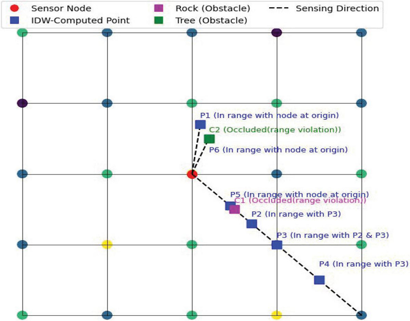
Figure 8 Generating a DEM and schematic deployment with grid.
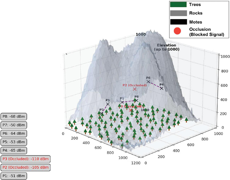
Figure 9 A sample terrain visualization showing occlusions in coverage.
Algorithm 1 outlines our proposed deployment approach. The algorithm starts with extracting and analyzing terrain data, creating contour and digital elevation maps, and applying path loss models, ultimately leading to identifying potential deployment locations. This is done by taking into account occlusions based on euclidean distance computed as a function of RSSI values that incorporate obstacles.
Algorithm 1 WSN deployment over irregular terrain with obstacles.
1: Input: Region of interest (RoI) coordinates
2: Output: Potential mote deployment locations
3: procedure WSNDEPLOYMENT(RoI)
4: Step 1: Extraction of region of interest and terrain analysis
5: Acquire high-resolution satellite imagery and elevation data from Google Earth
6: Select RoI and save in KML format
7: Convert KML to GPX format using TCX converter
8: Visualize GPX file using GPS visualizer to generate detailed maps and elevation profiles
9: Step 2: Creation of a contour map of the region of interest
10: Generate contour map from KML file using QUICKGRID
11: Step 3: Path loss model for obstacles
12: Define path loss models for different obstacles (trees, grass, rocks)
13: for each obstacle type (tree, grass, rock) do
14: Compute path loss using:
15: end for
16: Step 4: Creation of digital elevation map from contour map
17: Create DEM from contour map using grid representation
18: Step 5: Elevation estimation through IDW interpolation
19: for each unmeasured elevation point do
20: Compute elevation using IDW interpolation:
where
21: end for
22: Step 6: Identification of potential mote deployment locations
23: Choose a random origin point in DEM grid
24: for angle from 0 to 360 degrees in 1-degree increments do
25: Trace a straight line from origin at angle
26: for each point on the traced line do
27: Compute Euclidean distance from the previous deployment point
28: if then
29: Mark point as potential deployment location
30: else
31: Mark point as occluded
32: end if
33: end for
34: end for
35: end procedure
4 Results and Evaluation
4.1 Comparative Analysis with Existing 3D Regular/Irregular Methods
This section compares our proposed method with existing ones. To evaluate and compare these methods, we have created a simulation environment for our methodology as per the evaluation scenario (deployment area, communication range, etc.) defined by these methods with Python 3.10.11 on a notebook computer equipped with an Intel i7 12Th-gen processor, 16 GB of RAM, and a dedicated NVIDIA graphics card. We compare our proposed RSSI interpolation approach with existing methods comprising those by Li et al. [9], Udgata et al. [10], Fu et al. [11], Bhattacharyya et al. [12], Boualem et al. [15], Xiao et al. [16] and Liu et al. [17]. Tables 1, 2 and 3 include comparative analyses on the basis of coverage, motes required and complexity.
Table 1 Comparative analysis of RSSI interpolation with existing methods based on coverage
| Method | Terrain Size (m) | Comm. Range (m) | Coverage (%) |
| RSSI interpolation vs. Udgata et al. [10] | 17.60 | 100% in both | |
| RSSI interpolation vs. Liu et al. [17] | 60 | 100% in both | |
| RSSI interpolation vs. Bhattacharyya et al. [12] | 50 | 100% in both | |
| RSSI interpolation vs. Li et al. [9] | 25 | 100% vs. 47% | |
| RSSI interpolation vs. Xiao et al. [16] | 2 | 99.86% vs. 99.46% | |
| RSSI interpolation vs. Boualem et al. [15] | 50 | 100% in both | |
| RSSI interpolation vs. Fu et al. [11] | 5 | 100% in both | |
Li et al.: Li et al.’s method lacks a signal attenuation model for obstacle detection, and they haven’t assumed a proper three-dimensional terrain. In fact they have considered it as 2.5D; this makes it more suitable for applying it over a semi-regular surface rather than an irregular one with sharp elevation variations and obstacles. The complexity estimations are described in the “Complexity” column of Table 3. Here, represents the number of generations, is the number of particles, denotes the number of nodes, and denotes the sensing radius.
Udgata et al.: The method proposed by Udgata et al. employs image segmentation to generate irregular areas from rectangles but does not consider elevations or obstacles. The approach can be complex to scale for larger dimensions owing to the entire methodology being based on image segmentation. In the complexity analysis of this method, denotes the count of bees utilized in the artificial bee colony method and refers to the number of food patches selected for neighborhood exploration.
Table 2 Comparative analysis of RSSI interpolation with existing methods based on motes needed
| Method | Terrain Size (m) | Comm. Range (m) | Motes Needed |
| RSSI interpolation vs. Udgata et al. [10] | 17.60 | 10 vs. 16 | |
| RSSI interpolation vs. Liu et al. [17] | 60 | 300 vs. 400 | |
| RSSI interpolation vs. Bhattacharyya et al. [12] | 50 | 21 vs. 25 | |
| RSSI interpolation vs. Li et al. [9] | 25 | 14 vs. 20 | |
| RSSI interpolation vs. Xiao et al. [16] | 2 | 2947 vs. 4096 | |
| RSSI interpolation vs. Boualem et al. [15] | 50 | 4 vs. 99 (live) out of 200 | |
| RSSI interpolation vs. Fu et al. [11] | 5 | 274 vs. 444 | |
Table 3 Comparative analysis of RSSI interpolation with existing methods based on complexity
| Method | Terrain Size (m) | Comm. Range (m) | Complexity |
| RSSI interpolation vs. Udgata et al. [10] | 17.60 | vs. | |
| RSSI interpolation vs. Liu et al. [17] | 60 | vs. | |
| RSSI interpolation vs. Bhattacharyya et al. [12] | 50 | vs. | |
| RSSI interpolation vs. Li et al. [9] | 25 | vs. | |
| RSSI interpolation vs. Xiao et al. [16] | 2 | vs. | |
| RSSI interpolation vs. Boualem et al. [15] | 50 | vs. | |
| RSSI interpolation vs. Fu et al. [11] | 5 | vs. | |
Fu et al.: Fu et al.’s method does not account for different types of obstacles and the variations in elevation values are also not well defined for incorporating the signal attenuation model. Additionally, they have assumed the mote communication range to be 5 m, which is not practical in real terrains as the average range of such IoT devices is typically between 50 and 100 m.
Bhattacharyya et al.: Bhattacharyya et al. initiate mote deployment with a central server node referred as the fusion node and does not assume any geographical limitations. However, this method does not consider signal attenuation and skips deployment in areas obstructed by obstacles. In complexity analysis, the parameter denotes the distance between sensors.
Boualem et al.: Boualem et al. utilized a spiderweb technique for deploying motes on a regular 3D surface without considering obstacles. They evaluated coverage based on the minimum number of motes remaining active after an initial time period of 50 units.
Xiao et al.: Xiao et al. do not incorporate any obstacle estimation technique for their deployment method over varied terrains. In complexity estimations, represents the number of nodes deployed and indicates the iterations of the algorithm for each node.
Liu et al.: Liu et al.’s method focuses on irregular terrains but does not account for obstacles within these terrains. In complexity analysis, the parameters and are used to define the rows and columns of the grid used for deploying motes using a vertex-triangulation method.
4.2 Simulation Environment for Comparative Analysis with Various Regular Flat Surface Deployment Approaches
To validate the efficacy of the proposed deployment approach we compare it with existing regular/flat surface deployment techniques, namely, particle swarm optimization (PCO), ant colony optimization (ACO), Steiner tree, Delaunay’s triangulation, Voronoi polygon, genetic algorithm and random deployment. We have developed a simulation environment for this using Python 3.10.11 on a Notebook Computer equipped with an Intel i7 12th-gen processor, 16 GB RAM, and a dedicated NVIDIA graphics card. We simulated in this environment an irregular, obstacle ridden terrain of areas up to m with elevations going up to 1000 m. The terrain has randomly distributed obstacles comprising trees, natural tall grass, and rocks. These obstacles occupy areas that constitute 10%, 20%, 30%, 40%, 50%, and 60% of the total terrain area. The simulation environment comprises 100 random landscapes with varying percentage and distribution of obstacles. In addition to this, the environment considers the following varying mote communication ranges: 30 and 50 m. Using these large numbers and a variety of simulated terrains we are able to comprehensively compare the deployment efficacy of the various approaches.
4.2.1 Simulation Parameters for Comparison with Existing Regular/Flat Surface Deployment Techniques
Table 4 provides values for the simulation parameters that are used to implement existing regular/flat surface techniques for WSN deployment with which we compare our proposed method.
| Ant colony optimization (ACO) [27, 4] | |
| Parameter | Value |
| Number of ants | 100 |
| Pheromone influence | 1 |
| Evaporation rate | 0.3 |
| Particle swarm optimization (PSO) [28, 9] | |
| Parameter | Value |
| Number of particles | 100 |
| Inertia weight | 0.5 |
| Social and cognitive components | 1.5 each |
| Genetic algorithms (GA) [29] | |
| Parameter | Value |
| Population size | 100 |
| Crossover rate | 0.8 |
| Mutation rate | 0.2 |
| Simulation parameters for geometric algorithms | |
| Method | Parameters/values |
| Voronoi polygon | |
| Number of seeds/determined by nodes | |
| Boundary treatment/reflective | |
| Steiner tree | |
| Number of terminals/determined by nodes | |
| Edge weight computation/Euclidean distance, signal strength | |
| Delaunay triangulation | |
| Number of points/determined by nodes | |
| Triangulation method/incremental | |
4.3 Coverage vs. Obstacle Percentage with Varying Mote Communication Ranges
We use coverage as a measure for assessing the efficacy of the deployment technique in properly spreading the motes over the region of interest. It is mathematically defined as:
| Coverage | ||
| (6) |
A large percentage value of coverage implies that most of the motes deployed are effective and are not occluded by obstacles.
We evaluate the performance of the proposed approach, RSSI interpolation, for coverage against varying percentage of obstacles in the simulated terrain. We compare it with the seven existing deployment techniques mentioned earlier. As mentioned earlier, the comparison is conducted in a simulated environment generated for irregular terrains of size: m with an elevation going up to 1000 m. The communication range of the motes varies as 30 and 50 m, while the obstacle percentage varies between 10% and 60% of the terrain area. The obstacles include vegetation like trees and grass, and rocky formations.
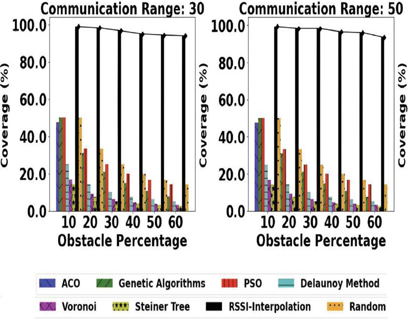
Figure 10 Coverage vs. obstacle percentage on terrain size 1000 with varying mote communication ranges.
The coverage as a percentage is shown in Figure 10 and clearly demonstrates the efficacy of the proposed RSSI interpolation method as compared to existing deployment techniques. Methods such as PSO, ACO, random deployment, and genetic algorithm initially converge well with a 10% obstacle density but struggle to maintain coverage as the obstacle size increases. The conventional methods, including Steiner tree, Delaunay, and Voronoi polygon, which rely on geometric principles for deployment, had significant shortcomings due to the unevenness of the terrain. As a special case, if we consider a scenario with no obstacles which implies that we are dealing with a smooth and regular 3D surface and thus there are no occluded points. In this situation a coverage of 100% can be attained. However, such ideal conditions are rare in real scenarios.
4.4 Normalized Motes required vs. Coverage on Varying Obstacle Percentage and varying Mote Communication Ranges for Terrain Size 1000
Normalized motes implies the number of motes required to achieve full coverage normalized for different techniques. The normalization exercise is imperative here as several existing techniques achieve a small percentage of coverage i.e. most of the region of interest is occluded by obstacles. Thus in these cases, the total number of motes required is small which is not a reflection of the superiority of the technique. Normalization compensates for this discrepancy and the number of normalized motes gives a clear picture of the efficacy of the technique.
| (7) |
This expression computes the number of motes needed to achieve 100% coverage of the terrain, Figure 11 clearly shows that the proposed approach, RSSI interpolation, requires the smallest normalized number of motes to achieve full coverage when compared with existing techniques for WSN deployment.
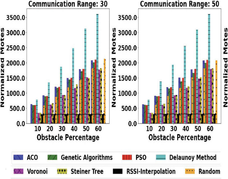
Figure 11 Normalized motes needed for full coverage vs. varying obstacle percentage and varying mote communication ranges.
4.5 Complexity Analysis
The algorithmic complexity of our proposed approach is computationally based on mote placement and obstacle handling tasks. For each of the landscapes having obstacles, the complexity will be . During mote placement each potential mote position requires the tasks of checking for coverage, performing IDW interpolation, and assessing obstacle interference. These operations have a complexity of per mote, where is the average number of motes required to achieve full coverage. Therefore for motes in each landscape, the overall complexity per landscape is . Thus, considering all landscapes the total complexity of the algorithm will be , which can be simplified to given a fixed number of landscapes .
4.5.1 Deployment Time Estimation Model
The total deployment time for placing motes across a landscape is represented as:
| (8) |
where:
• : Time required to verify coverage per obstacle for each mote.
• : Time needed to assess interference effects from each obstacle.
• : Fixed time for performing IDW interpolation per mote.
This model enables calculation of cumulative deployment time by combining time for obstacle-based coverage and interference checks with IDW interpolation for each mote. The total time scales with the number of motes, making it adaptable to diverse terrains with varying complexity.
Table 5 Region of interest within Melghat Tiger Reserve
| Parameter | Value |
| Latitude range | E to E |
| Longitude range | N to N |
| Elevation range | 585 to 630 m |
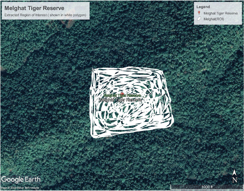
Figure 12 Google Earth image of the region of interest.
4.6 Deployment Results over an Extracted Real World Region of Interest
Study area: Melghat Tiger Reserve in District Amravati, Maharashtra, India The Melghat Tiger Reserve, located in the state of Maharashtra, India, is an ecologically rich and diverse habitat primarily known for its significant population of tigers. The topography of the reserve comprises of terrain that is uneven with a large number of obstacles in the form of grass, trees, rocks, and so on. We validate the efficacy of our proposed solution at the Melghat Tiger Reserve because of its diverse and uneven landscape and vegetation which comprehensively tests the working of the approach in a real world setting.
For our study, we extracted a specific region of interest within the Melghat Tiger Reserve using Google Earth. The extracted region is defined by the following geographical coordinates:
• Latitude: E to E
• Longitude: N to N.
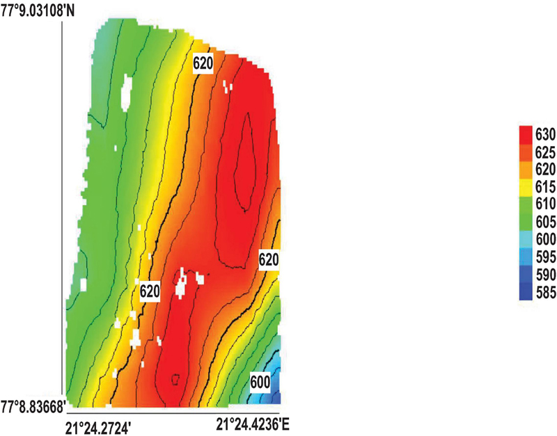
Figure 13 Contour map of the region of interest.
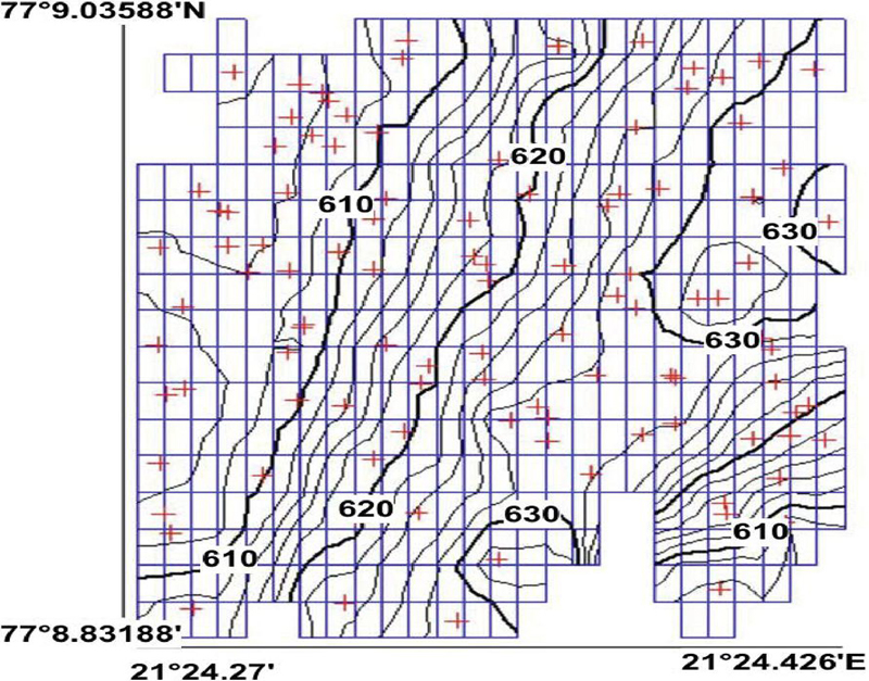
Figure 14 Corresponding DEM grid and the placed motes according to our proposed approach.
In this extracted region elevation values ranged between 585 and 630 m. This specific region within the Melghat Tiger Reserve extracted with google earth (specified in Figure 12) has been chosen as the potential area for our WSN deployment. Figure 13 presents a contour map of the target region, while Figure 14 illustrates its DEM overlaid with gridlines. Additionally, Figure 14 also depicts the points at which 105 WSN motes are deployed as determined by the proposed methodology. Using the execution obtained values s, s, s, and motes, substituting these into Equation 8 yields a calculated total deployment time of 294 seconds for our proposed approach.
5 Conclusion
WSN deployment over irregular terrains with obstacles such as vegetation and rocks is the central theme of this paper. Contemporary methods of deployment from the literature have been effective for simpler landscapes with regular topology, as well as for some irregular terrains without significant obstacles. These methods fail when implemented with the complexities of uneven terrains ridden with varying type obstacles. This work is an endeavor to bridge this important gap. The proposed approach comprises a series of steps from procuring images of landscapes, refining them, and making deployments taking into account the topography of the terrain and position to obstacles. The approach is compared with existing techniques of WSN deployment and is shown to be more effective in such irregular, obstacle ridden terrains. In response our methodology has proved to be more effective in such adverse complex irregular landscapes with obstacles. Our results indicate a significant reduction in occlusions compared to contemporary methods when implemented in such environmental settings. Additionally our approach required comparatively fewer motes to achieve extensive coverage even in complex environments with varying obstacle sizes. The practicality of our technique was further demonstrated through deployment over a real-world extracted region of interest.
Acknowledgments
We express our sincere thanks to the Ubiquitous Computing Laboratory (UbiComp) in the Department of Computer Science and Engineering at the Indian Institute of Technology Indore for their invaluable support in providing computing facilities.
Disclosure/Conflict of Interest
The authors declare no conflicts of interest.
References
[1] Wikipedia, WSN, https://en.wikipedia.org/wiki/Wireless\_sensor\_network, Last accessed on 2024/01/02.
[2] James Kennedy and Russell Eberhart. Particle swarm optimization. In Proceedings of ICNN’95 - International Conference on Neural Networks, volume 4, pages 1942–1948. IEEE, 1995.
[3] Raghavendra V Kulkarni and Ganesh Kumar Venayagamoorthy. Particle swarm optimization in wireless-sensor networks: A brief survey. IEEE Transactions on Systems, Man, and Cybernetics, Part C (Applications and Reviews), 41(2):262–267, 2010.
[4] Dina S. Deif and Yasser Gadallah. An ant colony optimization approach for the deployment of reliable wireless sensor networks. IEEE Access, 5:10744–10756, 2017.
[5] Shan You, Guanglin Zhang, and Demin Li. Coverage improvement strategy based on Voronoi for directional sensor networks. In Machine Learning and Intelligent Communications: First International Conference, MLICOM 2016, Shanghai, China, August 27-28, 2016, Revised Selected Papers 1, pages 247–256. Springer, 2017.
[6] Yifeng Tang, Dechang Huang, Rong Li, and Zhaodi Huang. A Non-Dominated Sorting Genetic Algorithm Based on Voronoi Diagram for Deployment of Wireless Sensor Networks on 3-D Terrains. Electronics, 11(19):3024, 2022. MDPI.
[7] Chun-Hsien Wu, Kuo-Chuan Lee, and Yeh-Ching Chung. A Delaunay triangulation based method for wireless sensor network deployment. Computer Communications, 30(14-15):2744–2752, 2007. Elsevier.
[8] Bo Yan. Node Deployment Algorithm Based on Improved Steiner Tree. International Journal of Multimedia and Ubiquitous Engineering, 10(7):329–338, 2015.
[9] Wenli Li. PSO based wireless sensor networks coverage optimization on DEMs. In Advanced Intelligent Computing Theories and Applications. With Aspects of Artificial Intelligence: 7th International Conference, ICIC 2011, Zhengzhou, China, August 11-14, 2011, Revised Selected Papers 7, pages 371–378. Springer, 2012.
[10] Siba K. Udgata, Samrat L. Sabat, and S. Mini. Sensor deployment in irregular terrain using artificial bee colony algorithm. In 2009 World Congress on Nature & Biologically Inspired Computing (NaBIC), pages 1309–1314. IEEE, 2009.
[11] Wendi Fu, Yan Yang, Guoqi Hong, and Jing Hou. WSN deployment strategy for real 3D terrain coverage based on greedy algorithm with DEM probability coverage model. Electronics, 10(16):2028, 2021. MDPI.
[12] Chandan Kr Bhattacharyya, Swapan Bhattacharya, and others. LDM (layered deployment model): A novel framework to deploy sensors in an irregular terrain. Wireless Sensor Network, 3(06):189, 2011. Scientific Research Publishing.
[13] Chien-Fu Cheng and Chu-Chiao Hsu. The deterministic sensor deployment problem for barrier coverage in WSNs with irregular shape areas. IEEE Sensors Journal, 22(3):2899–2911, 2021. IEEE.
[14] Yanzhi Du. Method for the optimal sensor deployment of WSNs in 3D terrain based on the DPSOVF algorithm. IEEE Access, 8:140806–140821, 2020. IEEE.
[15] Adda Boualem, Youcef Dahmani, Cyril De Runz, Marwane Ayaida, “Spiderweb strategy: application for area coverage with mobile sensor nodes in 3D wireless sensor network,” International Journal of Sensor Networks, vol. 29, no. 2, pp. 121–133, 2019. Inderscience Publishers (IEL).
[16] Fu Xiao, Xiekun Yang, Meng Yang, Lijuan Sun, Ruchuan Wang, Panlong Yang, “Surface coverage algorithm in directional sensor networks for three-dimensional complex terrains,” Tsinghua Science and Technology, vol. 21, no. 4, pp. 397–406, 2016. TUP.
[17] Liang Liu, Huadong Ma, “On coverage of wireless sensor networks for rolling terrains,” IEEE Transactions on Parallel and Distributed Systems, vol. 23, no. 1, pp. 118–125, 2011. IEEE.
[18] Tyagi, S., Srivastava, A.: Addressing WSN Deployments Over Obstacle Clad-Irregular Terrains. In the 4th International Workshop on Big Data Driven Edge Cloud Services (BECS 2024) Co-located with the 24th International Conference on Web Engineering (ICWE 2024), June 17–20, 2024, Tampere, Finland.
[19] Google. Google Earth 7.3. Available online: https://earth.google.com. Last accessed on 2024/01/02.
[20] TCX 2.0. TCX Converter. Available online: https://tcx-converter.software.informer.com/2.0. Last accessed on 2024/01/09.
[21] GPS Visualizer. GPS Visualizer. Available online: https://www.gpsvisualizer.com/. Last accessed on 2024/01/06.
[22] John Coulthard. Quick Grid 5.4.4. Available online: https://www.galiander.ca/quikgrid/. Last accessed on 2024/01/08.
[23] Tajudeen O. Olasupo, Abdulaziz Alsayyari, Carlos E. Otero, Kehinde O. Olasupo, and Ivica Kostanic. Empirical path loss models for low power wireless sensor nodes deployed on the ground in different terrains. In 2017 IEEE Jordan Conference on Applied Electrical Engineering and Computing Technologies (AEECT), pages 1–8. IEEE, 2017.
[24] Tajudeen O. Olasupo, Carlos E. Otero, Kehinde O. Olasupo, and Ivica Kostanic. Empirical path loss models for wireless sensor network deployments in short and tall natural grass environments. IEEE Transactions on Antennas and Propagation, 64(9):4012–4021, 2016. IEEE.
[25] Tajudeen Olawale Olasupo and Carlos E. Otero. The impacts of node orientation on radio propagation models for airborne-deployed sensor networks in large-scale tree vegetation terrains. IEEE Transactions on Systems, Man, and Cybernetics: Systems, 50(1):256–269, 2017. IEEE.
[26] Tajudeen Olawale Olasupo, Carlos Enrique Otero, Luis Daniel Otero, Kehinde Olumide Olasupo, and Ivica Kostanic. Path loss models for low-power, low-data rate sensor nodes for smart car parking systems. IEEE Transactions on Intelligent Transportation Systems, 19(6):1774–1783, 2017. IEEE.
[27] Mina Khoshrangbaf, Vahid Khalilpour Akram, and Moharram Challenger. Ant colony based coverage optimization in wireless sensor networks. In Annals of Computer Science and Information Systems, volume 32, pages 155–159, 2022.
[28] Yuhui Shi and Russell Eberhart, A modified particle swarm optimizer, in 1998 IEEE international conference on evolutionary computation proceedings. IEEE world congress on computational intelligence (Cat. No. 98TH8360), pages 69–73, IEEE, 1998.
[29] Jie Jia, Jian Chen, Guiran Chang, and Zhenhua Tan. Energy efficient coverage control in wireless sensor networks based on multi-objective genetic algorithm. Computers & Mathematics with Applications, 57(11-12):1756–1766, 2009. Elsevier.
Biographies

Shekhar Tyagi holds Bachelor’s and Master’s degrees in Computer Science and Engineering. He is currently pursuing his Doctoral degree in Computer Science and Engineering at the Indian Institute of Technology Indore. His research interests include edge computing, IoT security in resource-constrained environments, and machine learning.

Abhishek Srivastava is a Professor in the Discipline of Computer Science and Engineering at the Indian Institute of Technology Indore. He completed his Ph.D. in 2011 from the University of Alberta, Canada. Abhishek’s group at IIT Indore has been involved in research on service-oriented systems most commonly realized through web services. More recently, the group has been interested in applying these ideas in the realm of Internet of Things. The ideas explored include coming up with technology agnostic solutions for seamlessly linking heterogeneous IoT deployments across domains. Further, the group is also delving into utilizing machine learning adapted for constrained environments to effectively make sense of the huge amounts of data that emanate from the vast network of IoT deployments.
Journal of Web Engineering, Vol. 23_8, 1127–1154.
doi: 10.13052/jwe1540-9589.2384
© 2025 River Publishers