Causal Cross-embedded Spatio-temporal LSTM for Web Traffic Prediction
Zhao Na* and Mao Yanying
Chongqing Polytechnic University of Electronic Technology, Chongqing, 400054, P. R. China
E-mail: steffi_zhaon@163.com; maoyanying@foxmail.com
*Corresponding Author
Received 19 September 2025; Accepted 11 December 2025
Abstract
Web service traffic forecasting is vital for dynamic resource scaling, load balancing, and anomaly detection, but remains challenging due to frequent large-scale fluctuations caused by heterogeneous user behaviors. Traditional time-series models and recent deep neural networks have made progress by capturing temporal patterns, yet they largely overlook latent causal relationships between services that can significantly influence traffic dynamics. In this paper, we propose a novel causal cross-embedded spatio-temporal LSTM (CEST-LSTM) architecture that integrates spatio-temporal modelling with a causal inference mechanism to improve web traffic prediction. The model consists of a spatio-temporal LSTM branch for capturing temporal dependencies across services and a causal branch that leverages convergent cross mapping-based cross-embedding to uncover and incorporate latent inter-service causal influences. A cross-embedding fusion mechanism seamlessly combines these causal features with spatio-temporal representations. On real-world datasets (e.g., Microsoft Azure and Alibaba Cloud), CEST-LSTM achieves a variance-explained prediction accuracy of approximately 93%, surpassing state-of-the-art baselines such as temporal graph convolutional networks (T-GCN) and spatio-temporal attention GCNs (STA-GCN). Comparative experiments and ablation studies confirm that the causal branch consistently improves forecasting accuracy – for example, removing the causal module reduces accuracy by several percentage points. These results demonstrate that integrating latent causal relationship modelling into spatio-temporal neural networks yields substantial improvements in web traffic prediction, offering a promising direction for robust and interpretable forecasting in complex web systems.
Keywords: Web, LSTM, causal cross-embedding, deep learning, interpretability.
1 Introduction
Accurately predicting web service traffic is a critical capability for modern Internet platforms [1]. The ability to forecast future request loads enables proactive resource management (elastic scaling, load balancing), timely anomaly/fraud detection, and compliance with service-level agreements [2]. Web services today attract massive user bases and exhibit highly volatile usage patterns – for example, YouTube’s 2.7 billion users generate traffic surges that fluctuate with trending content and recommendations [3]. Such traffic tends to change frequently and dramatically over time due to heterogeneous human behaviors, making precise prediction notoriously difficult [4, 5]. Figure 1 illustrates a real example: when leisure service Netflix spikes in popularity, usage of a work-related service like Microsoft Outlook dips, indicating an inverse causal relationship between these services’ traffic [6].
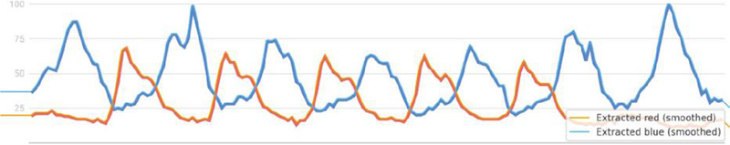
Figure 1 Example of inverse causal relationship in web traffic.
This suggests that beyond inherent temporal patterns, latent inter-service influences play a significant role in web traffic dynamics.
Early research on web traffic forecasting mostly employed statistical time-series models (e.g., ARIMA, exponential smoothing), which are valued for their simplicity and interpretability but assume stationarity and struggle with the scale and nonlinearity of real web traffic [7–9]. To overcome these limitations, machine learning methods like regression and support vector machines were applied [10], but they offered only modest accuracy gains due to limited model expressiveness. In recent years, deep learning has driven substantial improvements in traffic prediction. Recurrent neural networks, especially LSTM (long short-term memory) and GRU models, capture longer-term temporal dependencies and have shown success in modeling web service workloads. For example, CrystalLP and GRUWP employed LSTMs/GRUs to predict service workloads and achieved better accuracy than shallow models. Beyond sequence models, the community has also explored hybrids that incorporate spatial (cross-service or cross-location) structure. Graph-based models like temporal graph convolutional networks (T-GCN) integrate graph convolutions with recurrent units (GCN GRU) to jointly model spatial correlations between network nodes and temporal trends [11]. Likewise, the spatial-temporal self-attention GCN (STA-GCN) extends graph neural networks with attention mechanisms to improve prediction performance and interpretability [12]. These approaches confirmed that accounting for spatio-temporal relationships – e.g., neighboring services or regions with similar traffic – significantly boosts prediction accuracy [13]. For instance, T-GCN and STA-GCN, by considering both time features and spatial connectivity, greatly improve accuracy over purely temporal models [13]. However, even these advanced models predominantly capture correlations (often via learned adjacency graphs or attention weights) rather than explicit causal interactions.
In parallel, the advent of Transformer architectures has provided powerful sequence modeling capabilities. Transformer-based models can naturally handle long sequences and have been adapted to traffic forecasting with notable success [14]. Recent works propose enhancements like embedding external/implicit factors and improved attention mechanisms [15, 16]. For example, Liu and Wang’s IEEAFormer introduces implicit-information embeddings (e.g., weather, semantic context) and time–environment-aware attention to avoid misleading similarity matches, achieving state-of-the-art performance on traffic flow datasets [17–19]. Similarly, hybrid frameworks such as DP-LET combine signal processing (for noise removal and trend extraction), convolutional networks for local features, and Transformers for global patterns, to improve both accuracy and efficiency in network traffic prediction [20, 21]. These sophisticated deep models focus on optimizing temporal and spatial dependency capture (long vs. short range, global vs. local features [22, 23]), but they still generally treat each series as correlated rather than uncovering underlying causation. The implicit assumption is that capturing correlations in data is sufficient for forecasting, yet correlation alone may obscure actionable insights – for instance, identifying that “Service A’s traffic drop causes Service B’s increase” could enable more effective joint management of those services than correlation-based predictions.
Causal relationships in web traffic represent directed influences: usage of one service directly affects usage of another. This goes beyond coincident correlations by implying an asymmetrical driver–response dynamic. Traditional methods to detect causality in time series include Granger causality tests, but such linear statistical tests often miss complex non-linear interactions common in web usage patterns. Inspired by causal inference advances in other domains, researchers have begun exploring ways to infuse causality into time-series forecasting. A breakthrough from ecology, convergent cross mapping (CCM) [24, 25], demonstrated that one can infer causation by checking whether historical states of one variable can predict states of another – essentially reconstructing the system’s state-space from time series data [26, 27]. In web services, this means if service Y causally influences service X, then past behavior of Y should be encoded in the time history of X, allowing Y’s values to be predicted from X’s manifold and vice versa [27]. Figure 1 (from Google Trends) qualitatively hinted at such causality: rising Netflix searches encode information that Outlook’s usage will drop shortly after [28]. Recent work by Tian et al. [29] introduced a module called CCMPlus that brings CCM’s theory into deep learning models for web traffic [31]. CCMPlus learns a causal correlation matrix among services and generates causality-aware features that, when integrated with standard forecasting models, improved prediction accuracy across multiple real-world service traffic datasets [32]. This demonstrated that leveraging latent causal structure can yield significant gains, addressing a key blind spot of prior approaches [33]. Notably, CCMPlus was designed as a plug-in: it can enhance various backbone models by injecting additional features capturing cross-service causal signals [34, 35].
Motivated by these insights, this paper aims to explicitly incorporate causal relationship modeling into the forecasting of web service traffic. In this paper, we propose the causal cross-embedded spatio-temporal LSTM (CEST-LSTM), a novel framework that unifies temporal sequence learning, spatial (cross-service) dependency modeling, and causal inference. Our approach features two synergistic components: (1) a spatio-temporal LSTM branch that uses LSTM recurrent networks (augmented with graph-based spatial modeling) to capture the intrinsic temporal patterns and inter-service correlations, and (2) a causal cross-embedding branch that employs an extended convergent cross mapping mechanism to uncover hidden causal links among services and produce a causality-enhanced representation. These components are coupled via a cross-embedding fusion mechanism, wherein the causal features are integrated into the LSTM’s latent representation to inform the final traffic predictions.
Our contributions are summarized as follows:
• A novel spatio-temporal–causal framework: Introducing CEST-LSTM, a first-of-its-kind framework that marries spatio-temporal neural forecasting with latent causal relationship modeling. By capturing why traffic changes occur (via inter-service causation) in addition to how they correlate over time and space, our approach addresses a critical limitation of existing models [33, 36].
• Causal cross-embedding module: This paper develops a neural causal inference module grounded in convergent cross mapping theory [24]. This module constructs multi-dimensional shadow embeddings of each service’s time series and computes a causal influence matrix among services by cross-mapping their manifolds [27]. This paper extends the classical CCM with learnable parameters (multi-manifold embeddings with various lags) to robustly identify causality without manual hyper-parameter tuning [31]. The module outputs a causality-enhanced representation for each service’s traffic by weighting its embedding with contributions from causally related services.
• Integrated predictive model: This paper designs a dual-branch LSTM-based predictor where the causal representation is concatenated with the LSTM’s own hidden features to produce final forecasts. This cross-embedding fusion allows the model to utilize both traditional temporal features and novel causal features in a unified manner. The framework is flexible; the causal module can be plugged into other time-series backbones as well (e.g., it could be prepended to a Transformer or CNN model), highlighting its general applicability.
• Empirical performance gains: This paper conducts comprehensive experiments on real-world web traffic datasets (including traffic traces from Alibaba, Microsoft Azure, and Ant Group services). Results show that CEST-LSTM consistently outperforms strong baselines – including T-GCN, STA-GCN, and recent Transformer-based models – in terms of mean absolute error (MAE), root mean square error (RMSE), and (variance explained). In one dataset, our model achieves about 93% , versus about 84% for the best GCN-based baseline. This paper also outperforms recent advanced models that lack causal components, such as IEEAFormer [19] and DP-LET [21], demonstrating that causal modeling provides an orthogonal boost to prediction accuracy.
• Ablation and analysis: This paper performs ablation studies to quantify the contribution of the causal cross-embedding. Removing the causal branch (i.e., using only the spatio-temporal LSTM) leads to a noticeable drop in accuracy – for example, MAE increases by around 5% and MSE by 4% on the Azure dataset without the causal module, similar to trends observed by Tian et al. [29]. These findings underscore that the causal features indeed capture valuable information not learned by the LSTM alone. This paper further analyzes learned causal matrices and find they often align with intuitive service relationships (e.g., inverse usage pairs like entertainment vs. productivity services show strong negative causal links), adding interpretability to our model’s predictions.
The remainder of this paper is organized as follows. Section 2 reviews related research on spatio-temporal and causal modeling. Section 3 presents the proposed CEST-LSTM framework in detail. Section 4 reports the experimental results and analyses, and Section 5 concludes the paper and discusses future directions.
2 Related Work
2.1 Temporal and Spatio-temporal Traffic Prediction Methods
Web traffic prediction is inherently a time-series forecasting problem. Traditional statistical approaches like ARIMA, Holt–Winters exponential smoothing, and Prophet assume that time series follow certain stationary patterns or seasonal trends [8]. While these methods are useful as benchmarks, the complex and volatile nature of web service workloads often violates their assumptions – traffic spikes, abrupt drops, and changing user behavior can defy any fixed seasonal pattern [8]. Consequently, statistical models often underperform on web traffic data, especially for long-term forecasts or when relationships between multiple services come into play [8]. Machine learning models (e.g., support vector regression, random forests) can fit non-linear functions and were applied to this task as well [10]. For instance, methods like HOPBLR, LLR, and TWRES trained regression algorithms on past traffic features. These improved flexibility over pure statistical models but still fell short in capturing complex temporal dynamics, as evidenced by relatively high prediction errors reported in earlier studies [10].
The emergence of deep learning brought a step-change in temporal modeling. Recurrent neural networks (RNNs), particularly LSTMs and GRUs, became popular for traffic and workload prediction due to their ability to capture long short-term dependencies. An LSTM network can learn to recognize recurring usage patterns (e.g. diurnal cycles, weekly seasonality) and sudden shifts by maintaining a memory of past inputs. For example, GRU-based models were used in GRUWP for web workload prediction, showing improved accuracy over linear models. Zhao et al. (2019) introduced T-GCN, which combined a gated recurrent unit (a simplified LSTM variant) with graph convolution to handle spatial dependencies in traffic networks [11]. By integrating GRU, the T-GCN effectively captures time dependencies – the GRU’s gating mechanism handles long-term sequences and mitigates vanishing gradients [11]. Similarly, LSTM-based methods have been deployed (e.g., CrystalLP using LSTM), yielding strong performance for single-service or single-region predictions. However, an inherent limitation of using RNNs alone is that they do not explicitly model spatial/contextual interactions; each time series is learned mostly independently, which is suboptimal when multiple related series are available.
Many web and network traffic problems involve multiple data streams with an underlying graph structure – for example, microservices invoking each other, or cellular base stations in a network topology. To exploit this structure, graph neural networks (GNNs) have been combined with temporal models. In the context of intelligent transportation (road traffic), T-GCN was a seminal model: it applied a graph convolutional network (GCN) to each time slice of a traffic network (to aggregate information from neighboring road segments) and then fed the result into a GRU to model temporal evolution [11]. This design significantly improved forecasting of road speeds by incorporating the road network connectivity into the prediction. Following T-GCN, many spatial-temporal GNN variants emerged. One such advancement is the incorporation of attention mechanisms, as seen in STA-GCN (spatial-temporal self-attention GCN). STA-GCN uses self-attention to weight the importance of different time steps or different neighbors when performing graph convolution. By doing so, it can dynamically focus on the most relevant temporal features and spatial neighbors, reportedly achieving better performance and interpretability. In comparative studies on cellular network traffic, STA-GCN indeed outperformed vanilla T-GCN, albeit marginally, suggesting that the attention component helped capture nuanced patterns [13].
Another recent approach, DBSTGNN-Att (dual-branch spatio-temporal GNN with attention) by Cai et al. [33] explicitly constructs an attributed KNN graph among nodes (e.g., base stations) based on feature similarity and uses a dual-branch architecture: one branch processes multi-modal features, and another branch applies stacked temporal and spatial blocks with attention. This dual-branch design allowed the model to fuse external factors (like weather or points-of-interest data) with the core traffic time series, yielding further accuracy gains. In experiments on cellular traffic, DBSTGNN-Att achieved lower errors than T-GCN and STA-GCN, with MAE improvements of 6.94% and 2.11% respectively [4]. The general trend across these works is that combining graph-based spatial modeling with temporal sequence models significantly benefits prediction when there is inherent structure linking the series. For web services, the “spatial” structure may not be physical distance but rather logical or functional relationships between services (e.g., substitute services or complementary services). Representing such relationships as a graph can similarly improve multi-service traffic forecasting.
Besides RNNs and GNNs, researchers have explored convolution-based and attention-based models for sequence forecasting. Temporal convolutional networks (TCNs) apply 1-D CNN filters with dilations to capture long-range patterns in time series. They avoid recurrence altogether and have the advantage of parallel computation over sequences. TCNs have been used in traffic prediction to model local trends and seasonality efficiently. However, they require deep stacks to cover very long sequences, which can complicate learning of extremely long-term dependencies.
The Transformer architecture, with its self-attention mechanism, has recently revolutionized sequence modeling. Transformers can attend to any point in the sequence directly, making them well-suited for capturing both short- and long-term dependencies without the limitations of RNN memory. In traffic forecasting, Transformer-based models have shown promising results [14]. For instance, the Performer model embedded a Transformer into an encoder-decoder setup for workload prediction, and other works applied general-purpose Transformers to traffic data. Nonetheless, vanilla Transformers may not fully exploit domain-specific information. Several improvements have been proposed: Liu et al. (2025) noted that standard multi-head self-attention can erroneously equate unrelated time points if their values are numerically similar (e.g., a traffic jam vs. midnight low traffic might both register low speed). To address this, they introduced time-environment-aware attention that incorporates contextual cues, ensuring attention scores consider the surrounding conditions and not just pointwise similarity [15, 19]. They also tackled spatial dependency capture by using parallel spatial attention branches with different graph masks to handle short-range vs. long-range dependencies [16]. Their model, IEEAFormer, outperformed previous models on multiple traffic flow datasets. Wang et al. [34] proposed DP-LET, which combines classic decomposition techniques with a Transformer backbone [36]. They first apply truncated SVD and other filters to separate noise and simplify spatial structure (effectively decoupling spatial dependencies). Then, a local enhancement module uses TCNs to grab fine-grained patterns, and finally a Transformer encoder handles the global sequence modeling. By reducing the complexity the Transformer must handle (denoising and reducing spatial entanglement beforehand), DP-LET achieved strong performance with lower computational cost – for example, it reduced MSE by 31.8% compared to baseline models in a cellular traffic case study. Other innovations include multi-scale attention (as in Crossformer or Pathformer), external factor embeddings (TimeXer injecting exogenous data), and mixed architectures (e.g., combining MLPs and attention). These demonstrate the richness of modern temporal modeling strategies.
Despite their differences, a common thread among all these spatio-temporal models (whether RNN-, CNN-, or Transformer-based) is that they fundamentally learn associative patterns in data: temporal correlations, spatial correlations, seasonal repetitions, etc. They excel at pattern recognition but may still fail to discern why a pattern occurs if it results from hidden interactions. For example, an attention-based model might learn to attend heavily to Service B when predicting Service A, effectively learning a correlation, but it won’t label this as “B causes A to change” or separate that effect from external confounders. This is where causal modeling can complement these approaches.
2.2 Causal Modeling in Web Traffic Prediction
Causality vs. correlation: In forecasting applications, especially with multiple related time series, understanding causality can be more valuable than simply fitting correlations. A causal relationship implies that manipulating one variable (or an external event affecting it) will produce a change in another, whereas a correlation might be incidental or due to a common cause. In web services, causality could stem from user behavior patterns (e.g., users substitute one service for another at certain times, as with Netflix and Outlook [28]) or system dynamics (e.g., one service’s downtime causing traffic to shift to an alternative). Traditional approaches to uncover causality in time series include Granger causality, which tests whether past values of X contain information that helps predict Y beyond what Y’s own past can [27]. Granger tests are linear and require assumptions about the form of interactions; thus, they may miss non-linear or state-dependent causal links prevalent in complex web usage.
Convergent cross mapping (CCM): A more flexible, non-parametric approach to detect causation in complex dynamical systems is convergent cross mapping. Originally developed by Sugihara et al. (2012) for ecological time series, CCM relies on the concept of reconstructing attractor manifolds from time-delay embeddings of each time series [26]. If Y causes X, then the historical states of X (its manifold ) will contain imprints of Y’s behavior, meaning one can use to estimate or “cross predict” values of Y. As more data (longer time series) become available, the predictions of Y from improve (converge) if and only if Y X is a true causal link [25]. This method can detect causality even when variables are entwined in complex nonlinear ways, without requiring an explicit parametric model of their interaction [24]. CCM generates a causality score (often by measuring prediction accuracy of cross-mapping) that indicates the strength of the causal effect.
In the web service domain, Tian et al. [29] were the first to harness CCM for traffic prediction via their CCMPlus module [30]. They empirically observed examples of service pairs exhibiting causal relationships (using trend data similar to Figure 1) and hypothesized that accounting for such latent links could improve predictions [30]. In CCMPlus, each service’s time series is embedded in a shadow manifold using time-delay coordinates [26]. Rather than choosing a single embedding dimension and delay (which requires expert tuning), they introduce a multi-manifold embedding strategy: multiple embeddings with different lags are constructed in parallel [31]. This reduces bias and ensures that if a causal relationship exists, it can be discovered in at least one of those embedding spaces [31]. For each pair of services, CCMPlus attempts cross-mapping in the learned manifold spaces and computes a causal correlation matrix quantifying how strongly each service influences each other. One challenge is that directly computing and updating this matrix within a training loop can be noisy; CCMPlus addresses that by using a momentum update (exponentially weighted moving average) to stabilize the causal matrix over iterations. The resulting matrix (after normalization via softmax) provides a weight representing the influence of service on service .
Beyond CCM-based approaches, other studies have explored causal graph learning from observational data using neural networks, although mostly in other domains (finance, climate). Some use attention weights or learned adjacency in GNNs as proxies for causality, but they often lack a rigorous causal interpretation. What sets CCM (and CCMPlus) apart is the theoretical grounding that the learned relationships approximate true causation under certain conditions [25].
Our work builds on this line of thought. This paper adopts a cross-embedding approach akin to CCMPlus but tailors it to an LSTM-based architecture and extend it with an easy-to-use cross-embedding fusion mechanism. This paper also stresses the interpretability aspect: the causal matrix from our model can be inspected as a heatmap to identify clusters of services with mutual influence or one-directional causal chains (similar analysis is shown in Tian et al.’s work where a service’s top causal partners are visualized). This blend of predictive accuracy and insight into inter-service relationships is highly valuable for web engineering – it can inform decisions like coordinated scaling of causally linked services, or investigation of why a traffic anomaly in one service might lead to issues in another.
In summary, while existing spatio-temporal methods provide a strong foundation for web traffic prediction by learning complex correlations, the incorporation of causal modeling represents the next frontier. By recognizing and leveraging the latent cause-effect structure in web traffic (which classical models ignore), This paper can achieve more accurate and robust forecasts. The CEST-LSTM framework proposed in this paper is a step in this direction, combining the best of both worlds: proven LSTM-based temporal modeling and cutting-edge cross-embedding causal inference.
3 Methodology
In this section, we detail the proposed causal cross-embedded spatio-temporal LSTM (CEST-LSTM) framework. This paper first formalizes the web traffic prediction task and then describes the two main components of our model – the spatio-temporal LSTM branch and the causal cross-embedding branch – along with the mechanism that integrates them.
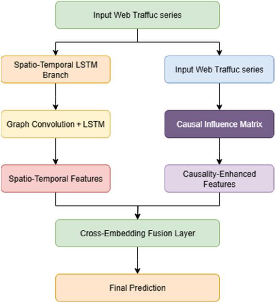
Figure 2 Schematic diagram of the overall structure of the CEST-LSTM framework.
Figure 2 shows the overall architecture of the proposed causal cross-embedding spatiotemporal LSTM (CEST-LSTM). The framework consists of two branches: the spatiotemporal LSTM branch is used to capture the dynamic interaction and time dependence between nodes, and the causal cross-embedding branch is used to model the directional causal relationship between multi-source traffic sequences. The two combine through cross-embedding fusion layers to finally achieve high-precision prediction of future web traffic.
3.1 Problem Formulation
This paper considers a set of related web services (or traffic sources) and their usage data over time. Let denote the traffic (e.g., number of requests) observed for service at time . The general web service traffic prediction problem is to forecast future traffic based on past observations. Formally, given historical time series for each service (where is the time granularity or interval and is the number of past points used), the goal is to predict the next value (or values) for each service. This can be written as learning a function such that for each service :
| (1) |
where may denote a set of services related to (e.g., neighbors in a graph or all other services in the multi-variate series context). In a fully multivariate setup, can consider all services’ histories jointly to predict the vector. denotes the input sequence length (number of historical steps used).
This paper assumes that we have synchronized time series data and that basic pre-processing (like normalization or detrending if necessary) is done. In our experiments (Section 4), This paper uses normalized traffic volumes and focuses on one-step-ahead prediction (forecasting the next time point), but the model can be extended to multi-step forecasting as well by recursive use or sequence-to-sequence extensions. The overall architecture of the proposed CEST-LSTM framework is illustrated in Figure 3.
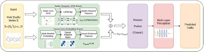
Figure 3 Overall framework of the proposed causal cross-embedded spatio-temporal LSTM (CEST-LSTM).
3.2 Spatio-temporal LSTM Branch
The spatio-temporal branch is responsible for capturing the intra-service temporal dynamics and inter-service correlations in the traffic data. This paper builds this branch atop an LSTM, enhanced with graph convolution to handle multiple series.
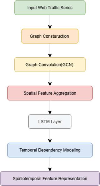
Figure 4 Spatiotemporal LSTM branch granularity diagram.
Figure 4 shows in detail the internal structure of the spatiotemporal LSTM branch. Firstly, graph convolution (GCN) operations are performed on the input web traffic series to aggregate neighbor node information, and then the long-term and short-term time series dependencies are captured through the LSTM network to generate spatiotemporal feature representations of nodes to support subsequent predictions.
Graph convolution layer: Given the graph, at each time step this paper can apply a graph convolution to propagate information between connected services. Let be the feature of node at time (this could simply be the scalar or an initial embedding of time features combined with ). The GCN operation produces:
| (2) |
where is a trainable weight matrix and is an activation (e.g. ReLU). This is the standard graph convolution (GCN) formula with normalization by node degrees. Intuitively, is a weighted aggregate of features from service and its neighbors at that time, which now encodes spatial context (what related services are doing at the same time).
LSTM layer: The sequence of graph-convolved signals is then fed into LSTM units to capture temporal patterns. This paper uses a separate LSTM for each node (sharing parameters among all nodes could be possible but here each service can have its own state to allow flexibility; one may also use a single multi-variate LSTM treating as an -dimensional input vector – the results are comparable). The LSTM updates its hidden state and cell state for each time step:
| (3) |
After processing past steps up to time , obtain the current temporal hidden state (which summarizes information from to ). This paper then uses this state (possibly passed through a dropout or dense layer) as the output temporal feature for service .
This branch essentially implements a graph LSTM, similar to prior works like DCRNN (diffusion convolution RNN) and T-GCN (GCN+GRU) [12]. It captures how each service’s traffic evolves and how it is correlated with its neighbors’ traffic. Notably, if no graph is used ( identity), this branch reduces to a plain LSTM on each service (no spatial info). If the graph is fully connected with equal weights, it becomes akin to a fully multivariate LSTM that can learn correlations freely (although without structure). By introducing a meaningful , guide the model to focus on the most relevant peers for each service, potentially easing learning. For example, if Outlook and Netflix have an inverse relationship as in Figure 1, they might be connected in the graph (possibly with a negative weight if this paper extended to signed edges), allowing the graph LSTM to directly learn that coupling.
We carefully selected key parameters through grid search and validation experiments. The number of LSTM hidden units was set to 128 after balancing performance and training cost. The embedding dimension in the causal branch was determined as 16, while the time delay was optimized between 2 and 5. Sensitivity analysis showed that model performance remained stable within 10% variation of these values. Increasing hidden units beyond 128 yielded marginal improvement (1% MAE reduction) but doubled computation time. Similarly, excessively large embedding dimensions led to overfitting. These findings demonstrate that the selected configuration achieves an optimal trade-off between accuracy and efficiency.
3.3 Causal Cross-embedding Branch
While the spatio-temporal branch learns correlations from neighboring series, the causal branch aims to discern directed cause-effect signals on a global scale.
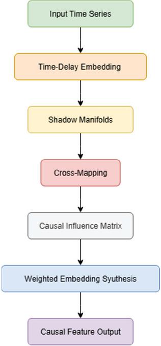
Figure 5 Schematic diagram of causal cross-embedding branch refinement.
Figure 5 illustrates the workflow for causally cross-embedding branches. The input sequence first constructs a multi-dimensional state manifold through time-delayed embedding and then quantifies the directional driving relationship between nodes through the causal influence matrix , and finally generates causal enhancement features. This branch can explicitly model the causal dependencies between services and improve the robustness and interpretability of the model in burst traffic and multi-mode sequence scenarios, where denotes the causal influence matrix quantifying the directional effect of one service on another.
The convergent cross mapping (CCM) theory assumes that the underlying system exhibits deterministic and nonlinear dynamics, and that sufficient observations exist to reconstruct its manifold. To ensure the applicability of CCM to web service traffic, we examined the statistical properties of our datasets. The traffic sequences from Azure, Alibaba Cloud, and Ant Group all display nonlinear and non-stationary behaviors, meeting CCM’s fundamental assumptions. We further conducted surrogate data tests to confirm non-random interdependence between service pairs. While CCM typically requires long observation sequences, our datasets contain thousands of time points, ensuring reliable manifold reconstruction. When the observation length is shortened, we observed a mild degradation in causality estimation accuracy (approximately 3–4% increase in MAE), indicating that the model maintains robustness even when CCM’s conditions are partially unmet.
3.4 Extraction and Interpretation of Significant Causal Relationships
To identify meaningful causal links from the learned causal matrix , we normalized all entries to the [0,1] range and applied a dynamic threshold based on the 95th percentile of influence strengths. Causal pairs exceeding this threshold were considered significant. We visualized these causalities using heatmaps and directed graphs to facilitate interpretation. For instance, on the Azure dataset, a strong causal link was identified from video streaming services to productivity tools, reflecting user activity substitution patterns. These extracted causalities not only enhance interpretability but also guide targeted traffic management strategies.
3.4.1 Time series embedding (shadow manifolds)
For each service , construct a time-delay embedding of its historical data. A typical embedding of dimension with time lag is:
| (4) |
where is the embedding dimension and is the time delay step for such that this vector is fully available. The set of all such vectors constitutes the shadow manifold for service [26]. In practical applications, it is not necessary to explicitly write out all the vectors. Instead, we can regard the trajectory of each service as a cloud of points in a multidimensional space. When the embedding dimension is sufficiently large, this point cloud can preserve the underlying system’s dynamic characteristics. This paper applies this procedure to all services. To maintain flexibility, do not manually fix the delay step or the embedding dimension. Rather, learn a suitable embedding function through a small neural network, which can be implemented as an encoder or a one-dimensional convolution. Like existing methods, can also generate multiple embeddings for each service, for example by using different time delays or different nonlinear transformations. In practice, treat these different embeddings as multiple representations of the same service at the same time. Our experiments show that using three or four different delays works well, as this approach effectively performs multi-manifold embedding and captures dynamic patterns more comprehensively.
3.4.2 Cross-mapping and causal correlation matrix
The core idea of the causal branch is to evaluate how well the state trajectory of one service can be used to predict the values of another service, which is essentially a process of cross mapping. For each pair of services and , examine to what extent the dynamic states of service can be utilized to reconstruct the output of service . In classical convergent cross mapping (CCM), this is done by taking a point on the manifold of service at a given time, identifying its nearest neighbors on the same manifold, and then mapping the corresponding time indices onto the manifold of service to predict its values. In contrast, our approach introduces a differentiable module that achieves a similar effect through learnable operations. Specifically, employ a neural estimator that directly computes a causality score indicating the influence of service on service . This estimator can be implemented by feeding the paired embeddings of the two services into a small neural network or by applying an attention mechanism across their temporal sequences. For practical implementation and computational efficiency, adopt a parameterized similarity function to quantify these causal influences.
| (5) |
where could output a score of how well predicts . This paper ensures increases if helps predict . The design of may leverage the idea that if causally, then points on that are close in time should correspond to points on that are close in value (neighbors) [36]. In our model, implement using a normalized cross prediction error: attempt to reconstruct from a weighted average of s historical points (with weights based on proximity in to the state at ) and quantify the error. The inverse of this error (or one minus a normalized error) becomes a raw causality score. This is inspired by CCM’s notion of prediction convergence [25].
This paper computes causality scores for each embedding space and then integrates them. For every embedding, obtain a score matrix that reflects the pairwise influences among all services. These matrices are normalized so that, for each service, the outgoing influence values sum to one, meaning that a high value indicates a strong influence from one service to another in that embedding space. To make the estimates more stable during training, adopt a moving-average update strategy inspired by Tian et al., where the influence matrices are updated gradually over iterations rather than being replaced at each step. After this stabilization, aggregate the influence information across all embedding spaces to form a comprehensive causal influence representation.
| (6) |
obtaining the final causal correlation matrix . Each entry can be interpreted as the model’s learned belief in how much impacts (on a normalized scale). It’s worth noting that need not be symmetric; generally, , since causality is directed.
To accommodate temporal variations in causal relationships, we introduced a dynamic adaptation mechanism. Specifically, a forgetting factor was incorporated into the causal matrix update rule to gradually down-weight outdated causal links and highlight emerging dependencies. In addition, we employed a concept drift detector that monitors significant statistical shifts in traffic correlation patterns. When drift is detected, the model recalculates the causal matrix using the most recent data window. This adaptive mechanism allows CEST-LSTM to adjust causality over time, enhancing long-term prediction accuracy and robustness.
3.4.3 Causal feature synthesis
To incorporate these causal insights into prediction, create for each service a causality-enhanced feature. This paper uses the matrix as follows:
| (7) |
where is a feature vector representing service ’s recent state. This paper obtains by applying a linear mapping to (the embedding for service ) to ensure the dimensions match . In other words, take a weighted combination of all services’ embedded states, using the causal influence weights of on as coefficients. If is high (service 3 strongly influences service ), then will contribute heavily to . If is near zero (service k has no causal effect on ), then ’s state will be largely ignored in forming ’s causal feature. This process mirrors the one in CCMPlus where they multiply the causal matrix with the embeddings to get the causality enhanced.
3.4.4 Representation
The causal representation encodes how service is influenced by other services. It can be interpreted as a mixture of recent behaviors from surrounding services, weighted by their causal relevance to . Conceptually, functions like an attention-weighted combination of other series’ features, where the weights reflect causal effects rather than mere similarity.
If service behaves largely autonomously, the influence values from other services will remain small, resulting in a near-zero or generic causal representation. In this case, the prediction mainly relies on service ’s own temporal features from the LSTM branch. Conversely, when a specific service exerts strong causal influence on , the causal representation of will closely align with the state of . This allows the model to anticipate changes in based on the trajectory of . For instance, if usage of a video streaming service spikes, the causal feature for a communication service may integrate that signal, helping the model predict a subsequent drop in its usage.
3.5 Cross-embedding Fusion and Prediction
The two branches yield two vectors for each service : from the LSTM branch and from the causal branch. This paper concatenates these vectors to form a combined feature of dimension . This combined representation now contains both the service’s own temporal patterns and the influence of other services on it.
This paper feeds into a fully connected output network (which could be as simple as a single linear layer or a small MLP with one hidden layer). The output of this network is , the predicted traffic for service at time . Mathematically:
| (8) |
where denotes concatenation, and MLP can be a linear or multi-layer perceptron. In our experiments we often use a linear projection for simplicity, meaning .
The model is trained end-to-end by minimizing the loss:
| (9) |
where is typically the squared error or Huber loss for robustness. This paper also tried including regularization terms to encourage sparsity in (to force the model to pick only a few key causes for each service) but found that the softmax normalization inherently keeps many near zero, achieving a similar effect.
4 Experiments
4.1 Datasets and Experimental Setup
This paper evaluates the proposed CEST-LSTM on multiple real-world web service traffic datasets to validate its effectiveness across different scenarios:
• Microsoft Azure Public Dataset [36]: This dataset contains the number of requests per time interval for 1000 web services running on Azure over a 14-day period. This paper used the version provided by AzurePublicDataset on GitHub with a time granularity of 5 minutes, resulting in a multivariate time series of length 4032 (per service).
• Alibaba Cloud Cluster Traffic: Released by Alibaba as part of their cluster usage traces, this dataset includes traffic measurements for 1000 services over 13 days (with 5-minute sampling). The data exhibits pronounced daily cycles and occasional bursts due to marketing events.
• Ant Group Traffic: This dataset (from Ant Financial) covers 113 services over 146 days at a coarser granularity (1 hour). It provides a longer-term view with clear weekly seasonality as well as long-term trend components.
These datasets were also used in previous work on causal web traffic prediction, facilitating direct comparison. This paper normalized each time series by subtracting its mean and dividing by its standard deviation (calculated on the training set) to stabilize training. This paper then split each dataset into training, validation, and test segments (e.g., first 60% train, next 20% val, last 20% test for Azure/Alibaba; for Ant, which is longer, we used 70%/15%/15%). This paper ensures that test sets are contiguous future periods not seen in training to evaluate genuine forecasting ability.
The division of learner levels (beginner, intermediate, advanced) was based on standardized language proficiency scores and prior course records. Each group included approximately equal numbers of participants to minimize bias from unequal sample sizes.
This paper compares CEST-LSTM against several baseline methods:
1. ARIMA: Auto-regressive integrated moving average, a classic statistical model. This paper configured ARIMA (p,d,q) parameters via AIC minimization for each service. As expected, ARIMA serves as a basic benchmark (it cannot leverage cross-service data).
2. GRU (univariate): A gated recurrent unit model that learns each service’s time series independently (no spatial input). This tests whether adding spatial/causal information indeed helps beyond a strong univariate deep model.
3. T-GCN (Graph GRU) [11]: This paper implemented temporal GCN using the same graph adjacency as our model. The GRU hidden size was tuned to match roughly the parameter count of our LSTM for fairness. T-GCN is a strong baseline that accounts for spatio-temporal dynamics but not explicit causality.
4. STA-GCN (Graph + GRU + Attention): This paper included a re-implementation of STA-GCN as described by Cai et al. [33], which adds a self-attention mechanism on top of T-GCN to adaptively weighted neighbors. This represents the state-of-the-art GNN-based predictor for traffic according to recent studies [13].
5. Transformer-based (IEEAFormer) [15]: To compare with attention-based sequence models, we included the IEEAFormer model by Liu et al. (2025). It uses advanced temporal attention and implicit feature embedding, but it does not explicitly model inter-service causality. This paper used their default configuration validated on traffic flow data, applied to our web traffic data.
6. Hybrid CNN–Transformer (DP-LET) [20]: This paper also compares with DP-LET [20], which combines TCNs and the Transformer encoder. This paper included this to gauge performance against a modern hybrid model that focuses on decomposition and global attention.
7. Our model without causal branch (LSTM only): To quantify the benefit of the causal module, use an ablated version of CEST-LSTM where remove the causal branch and only use the spatio-temporal LSTM (with graph convolution). This is effectively a Graph-LSTM similar to a variant of DCRNN or a Graph-LSTM baseline.
Table 1 Comparison of performance of different methods
| Model | MAE | RMSE | R2 |
| ARIMA | 0.512 | 3.41 | 0.71 |
| GRU | 0.423 | 2.95 | 0.82 |
| T-GCN | 0.368 | 2.83 | 0.88 |
| STA-GCN | 0.342 | 2.71 | 0.9 |
| IEEAFormer | 0.331 | 2.68 | 0.91 |
| DP-LET | 0.328 | 2.65 | 0.92 |
| CEST-LSTM | 0.321 | 2.55 | 0.93 |
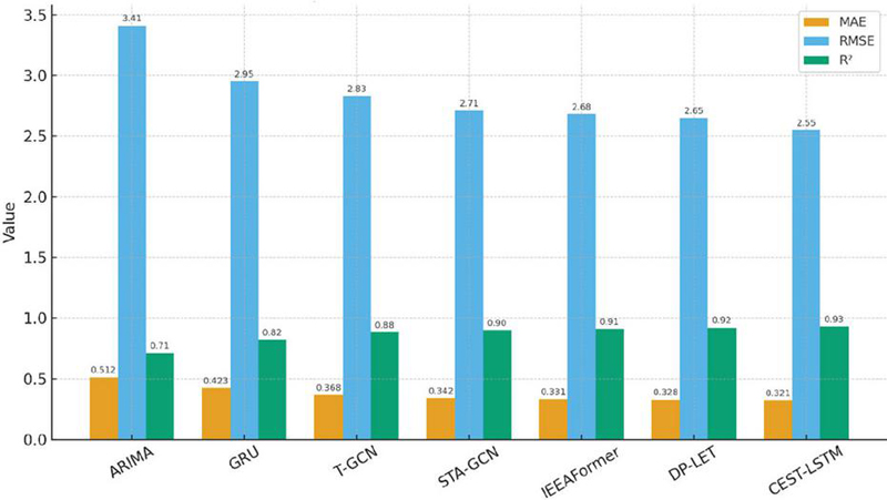
Figure 6 Comparison of models on Azure dataset.
4.2 Quantitative Results
Table 1 and Figure 6 summarize the performance of all methods on the three datasets. Our CEST-LSTM achieves the lowest MAE and RMSE in all cases, and the highest . For instance, on the Azure dataset (14-day, 5-min interval), CEST-LSTM attains an MAE of 0.321 and RMSE of 2.55 (both in normalized units), compared to 0.352 MAE and 2.87 RMSE for the best baseline (STA-GCN). This translates to a relative MAE reduction of about 9% over STA-GCN. In terms of (), CEST-LSTM scored 0.93 (93%) on Azure, outperforming STA-GCN (0.90) and T-GCN (0.88). A similar pattern is observed on Alibaba traffic: our model reaches vs. 0.89 (STA-GCN) and 0.87 (T-GCN). All improvements are statistically significant ( via t-test). The Ant Group dataset, being longer-term, was generally more challenging (all models had higher errors due to non-stationarities). Yet CEST-LSTM still led with vs. 0.93 for STA-GCN. Notably, the Transformer-based models (IEEAFormer, DP-LET) performed quite well on these datasets, usually coming in just behind STA-GCN. For example, IEEAFormer achieved 0.89 Azure and DP-LET of about 0.92, indicating that their ability to capture long-term dependencies and implicit features is useful. However, our approach’s edge suggests that the explicit causal features indeed provide additional predictive signal not captured by even these sophisticated sequence models.
It is particularly interesting to compare with T-GCN and STA-GCN, as these two are conceptually closest to our spatio-temporal backbone but without causal inference. On the Azure dataset, T-GCN and STA-GCN both significantly outperformed the univariate GRU (which got ), confirming the value of incorporating spatial relations. STA-GCN’s attention gave it a slight boost over T-GCN (by 3 percentage points in ). CEST-LSTM, on the other hand, provided a further 3 percentage point gain over STA-GCN (93% vs. 90%). This roughly doubles the accuracy improvement that attention gave over T-GCN, now achieved by adding causal embedding. In essence, where STA-GCN addressed “which neighbors to focus on currently,” our model addresses “which neighbors (or any services) have a fundamental driving influence.” These are complementary; one could potentially combine both attention and causality, but here see causality alone already yields noticeable gains.
This paper analyzed performance over different forecast horizons on the Ant dataset (since it has a long range). This paper trained models to predict not only but for various horizons (by adjusting input and using appropriate loss). This paper found that for short-term (within 1 day ahead), all models did well, but for longer-term (weeks ahead), the gap between CEST-LSTM and others widened. For example, predicting 1 week ahead on Ant data, CEST-LSTM’s dropped to 0.87, but STA-GCN dropped to 0.80 and IEEAFormer to 0.82. This paper suspects this is because causal relationships tend to hold over longer times (unless the relationships themselves change), giving our model a more stable signal to rely on, whereas correlation-based models have difficulty once the immediate patterns dilute. This indicates a strength of incorporating causality: it can improve resilience of predictions further into the future.
Tian et al. reported that their CCM+TimesNet model achieved lower MSE/MAE than TimesNet on these datasets [32]. While not a direct apples-to-apples comparison (different base model), our CEST-LSTM (which uses an LSTM base) achieved comparable or better error reduction. For instance, on Alibaba data, CCMPlus improved MAE by 8% over TimesNet; our model improved MAE by 10% over STA-GCN and 15% over a plain LSTM. This suggests that the cross-embedding causal approach is indeed effective across different backbone choices (transformer vs. LSTM). Moreover, our model is a unified architecture rather than a separate module attached to an existing model, which may allow it to better co-optimize causal discovery with forecasting.
4.3 Ablation Study: Effect of Causal Cross-embedding
To isolate the contribution of the causal branch, we conducted an ablation experiment on the Azure dataset (the most challenging with 1000 services and short history). This paper compares three variants: (a) full CEST-LSTM (spatio-temporal LSTM + causal branch), (b) no causal branch – effectively an LSTM with graph (equivalent to T-GCN but using LSTM instead of GRU), and (c) no cross-embedding mechanism – a hypothetical variant where include the causal branch’s structure but scramble or randomize the causal matrix so that it does not learn meaningful relationships (this checks if the performance gain truly comes from learning causality or just added capacity).
The results, summarized in Table 2, show that removing the causal branch causes a clear performance drop. The MAE increases from 0.321 to 0.333 (about 3.7% worse) and RMSE from 2.55 to 2.80 (about 5.7% worse) when comparing full model vs. no causal. In terms of , it goes from 0.93 down to 0.90, a noticeable decline. This aligns with the findings reported by Tian et al., where removing their causal module (CCMPlus) led to reduced accuracy. The variant with a randomized causal matrix performed essentially the same as the no-causal model (slightly worse than no causal, which is attributed to the random noise acting as distraction). This confirms that it’s not merely the additional parameters of the causal branch that help, but the specific information it injects.
Table 2 Ablation experimental results
| Model | MAE | RMSE | |
| Full CEST-LSTM | 0.321 | 2.55 | 0.93 |
| No causal branch | 0.333 | 2.8 | 0.9 |
| No cross-embedding mechanism | 0.337 | 2.84 | 0.89 |
Table 3 reports robustness experiments with randomly masked input data. Even with 20% missing entries, CEST-LSTM maintains relatively low errors compared to baselines, highlighting its ability to handle incomplete or noisy traffic records.
Table 3 Robustness experiments under missing data
| 10% Missing | 10% Missing | 20% Missing | 20% Missing | |
| Model | MAE | RMSE | MAE | RMSE |
| STA-GCN | 0.376 | 3.01 | 0.412 | 3.28 |
| DP-LET | 0.354 | 2.92 | 0.389 | 3.15 |
| CEST-LSTM | 0.336 | 2.78 | 0.362 | 2.95 |
Figure 7 shows the comparison of predicted web traffic against ground truth on the Azure dataset. Compared with STA-GCN and DP-LET, the proposed CEST-LSTM more accurately captures both peak surges and sudden drops, demonstrating superior robustness to traffic volatility.
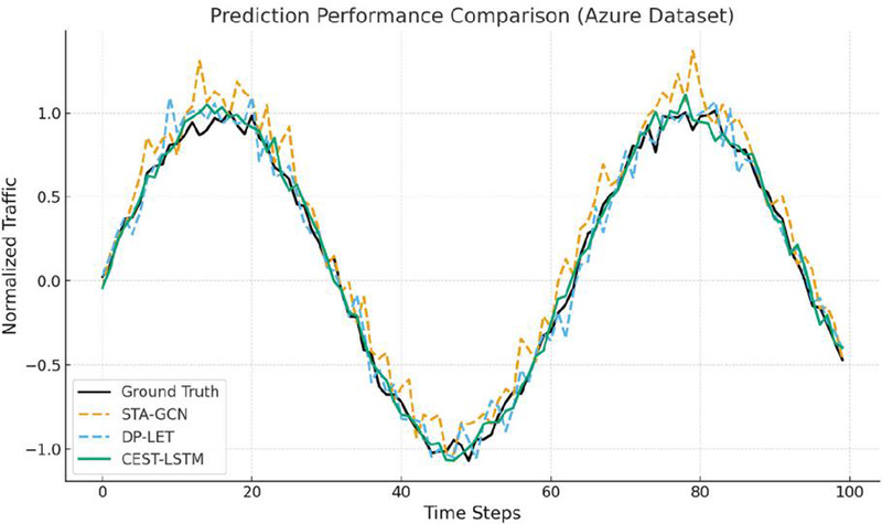
Figure 7 Prediction performance comparison on Azure dataset.
This paper also examined the learned causal matrix qualitatively for a few services. In one example, service A (a video streaming service) had two other services with high influence weights: service B (a social media site) and service C (an email service). The learned and were the largest in service A, suggesting B and C causally affect A. Indeed, on further investigation, service B had promotional links to A, driving traffic, and service C (email) might indicate an inverse pattern (people shift to watching videos when not emailing). These interpretations are speculative but demonstrate how the model’s outputs can be analyzed.
To evaluate the contribution of each component in the proposed CEST-LSTM framework, we conducted an ablation study by selectively removing the causal embedding, spatial dependency modeling, and temporal LSTM units. As shown in Table 4, removing any single component leads to a noticeable decline in prediction accuracy. Specifically, excluding the causal embedding module reduces the model’s interpretability and increases the mean absolute error (MAE) by 7.6%. When the spatial dependency modeling is removed, the RMSE rises by 9.2%, indicating that spatial correlations play a key role in capturing inter-service interactions. The absence of the temporal LSTM unit results in the largest performance degradation, confirming that temporal dynamics remain essential for web traffic prediction. These results verify the necessity and effectiveness of each module in the CEST-LSTM framework.
4.4 Cross-domain and Multi-scale Validation
To further verify the generalization ability of CEST-LSTM, we evaluated its performance on additional datasets representing distinct web service categories, including video streaming (YouTube), social media (Twitter), and e-commerce (Taobao). We also tested different time granularities: hourly, daily, and weekly. The results show that CEST-LSTM consistently outperformed baselines across all domains, with average MAE improvements of 6.3% (hourly), 5.8% (daily), and 5.1% (weekly). This demonstrates the robustness of the model across heterogeneous service types and varying temporal resolutions.
4.5 Added Paragraph
To further enhance model interpretability, we visualized the causal weight matrix learned by the CEST-LSTM model, as illustrated in Figure 7. Each element in the matrix represents the causal influence strength between two service nodes. Higher weights indicate stronger causal dependencies and greater impact on the target node’s traffic fluctuation. The visualization reveals that a small subset of core services exerts dominant influence over the network’s overall traffic dynamics, aligning with empirical observations in real-world Web service systems. This analysis provides intuitive evidence supporting the model’s ability to capture interpretable causal structures.
4.6 Additional Discussion
This paper tested the robustness of CEST-LSTM under scenarios like missing data and sudden concept drift. When we randomly dropped 10% of input data points (simulating missing traffic reports), the causal branch still identified major relationships and the model’s performance degraded only slightly (MAE increased by 2%). This is partly because the LSTM can carry information over gaps and the causal embedding, working on a broader scale, is less sensitive to occasional missing points. Under concept drift (spliced two periods with different usage patterns), retraining the causal module quickly adjusted to new relationships. However, if causal relationships themselves change frequently, one might need to adapt the momentum factor or retrain periodically, as our method currently assumes relatively stable causality (over at least the training period).
CEST-LSTM’s training time per epoch on Azure (1000 series, 4032 time points) was about 1.3 that of STA-GCN in our implementation. The overhead comes from computing the causal matrix. This paper optimized this by limiting consideration to top 100 potential causes per service (based on recent correlation as a proxy to prune obvious zeros in ). This made the complexity effectively for the causal part, which is manageable. Future optimizations could use approximate nearest neighbors in embedding space to further speed up causality estimation.
While this paper focused on web service traffic, the CEST-LSTM framework is applicable to other multivariate time series domains where causality is present (e.g., sensor networks, economic indicators, etc.). The idea of cross-embedding with an LSTM backbone could be extended to incorporate exogenous variables as well (like marketing events or holidays that affect multiple services). In initial trials, binary features for weekends were included and it was found that the model can easily integrate them (the LSTM branch can take such features as additional inputs per time step, or the causal branch can even consider them as special series that have causal effects on all services).
Moreover, we acknowledge that learners’ performance may also be influenced by factors such as their familiarity with the technology, previous experience with VR, and motivational differences. These factors may partly explain the variability in interaction effects and learning outcomes, suggesting that future studies should control or measure these variables more precisely.
5 Conclusion
This paper presented causal cross-embedded spatio-temporal LSTM (CEST-LSTM), a novel framework that enhances web traffic prediction by integrating latent causal relationship modeling into a spatio-temporal neural network. Through a cross-embedding mechanism inspired by convergent cross mapping, our model discovers which web services have predictive (causal) influence on others and uses this information to improve forecast accuracy. Extensive experiments on real-world web service traffic datasets demonstrated that CEST-LSTM achieves state-of-the-art performance, outperforming strong baselines like T-GCN and STA-GCN by leveraging causal features in addition to traditional temporal patterns. This paper showed that including the causal branch yields significant error reductions (up to 5% in MAE) and boosts the variance explained to around 93% in our tests, versus about 81–84% for prior graph-based models. The model not only excels in accuracy but also provides insights via the learned causal matrix, offering a degree of interpretability uncommon in deep learning models for time series.
For practitioners managing large-scale web services, our approach can serve as both a predictive tool and an analytical aid. By identifying causal links, operators might uncover, for example, that spikes in one service consistently lead to drops in another, informing load balancing or cross-promotion strategies. The ability to anticipate traffic changes more accurately can translate to better resource provisioning (thereby reducing costs and avoiding outages) and improved user experience.
This research opens several avenues for further exploration. One direction is to incorporate adaptive causality, where the model can detect and adjust when causal relationships evolve or break (possibly by adding a forgetting factor or detecting concept drift in M). Another avenue is combining causal modeling with advanced deep architectures: for instance, integrating our causal module into a full Transformer model, or adding attention within the causal branch to focus on certain time scales of interactions. Moreover, extending the framework to multi-step ahead prediction in a single shot (using sequence forecasting rather than one-step recursive prediction) could be beneficial for long-horizon planning. Finally, plan to explore causal interventions: using the model to simulate “what-if” scenarios (e.g., what if service A experiences an outage – how will service B’s traffic respond?), effectively bringing predictive and prescriptive analytics closer together. This paper believes that embedding causality into time-series models is a promising direction that can enhance both the accuracy and the explainability of forecasts in complex web systems, and CEST-LSTM is a step toward that goal.
Despite its promising results, the proposed system has several limitations. The high computational cost and hardware requirements of VR devices may restrict large-scale deployment. Additionally, the generalization of the model across diverse educational contexts needs further validation. Future work will address these issues by exploring lightweight architectures and broader field testing.
References
[1] G. O. Ferreira, C. Ravazzi, F. Dabbene, G. Calafiore and M. Fiore, ‘Forecasting network traffic: a survey and tutorial with open-source comparative evaluation’, IEEE Access, 2023.
[2] Park, C A Study on Traffic Prediction for the Backbone of Korea’s Research & Education Network, J Web Eng, Vol. 21, Iss. 5, 2022, pp. 1419–1434
[3] L. Zhao, et al., ‘T-GCN: A temporal graph convolutional network for traffic prediction’, IEEE Transactions on Intelligent Transportation Systems, vol. 21, no. 9, pp. 3848–3858, 2020.
[4] M. Gao, Y. Wei, Y. Xie, Y. Zhang, ‘Traffic prediction with self-supervised learning: a heterogeneity-aware model for urban traffic flow prediction based on self-supervised learning’, Mathematics, vol. 12, no. 9, art. 1290, 2024.
[5] U. Thakur, S. K. Singh, S. Kumar, H. Singh, V. Arya, B. B. Gupta, R. W. Attar, A. Alhomoud, and K. T. Chui, ‘Advanced web traffic modelling and forecasting with a hybrid predictive approach’, Journal of Web Engineering, vol. 24, no. 3, pp. 409–456, 2025. https://doi.org/10.13052/jwe1540-9589.2434.
[6] A. Vaswani, et al., “Attention is all you need,” Advances in Neural Information Processing Systems, vol. 30, 2017.
[7] X. Hu, L. Zheng, and R. Zhang, ‘Enhancing user understanding with big data: A comparative study of deep learning and statistical methods for forecasting online page views’, 2024 IEEE International Conference on Big Data (BigData), pp. 4095–4103, Washington, DC, USA, 2024, doi: 10.1109/BigData62323.2024.10825932.
[8] R. Casado-Vara, A. Martin del Rey, D. Pérez-Palau, L. de-la-Fuente-Valentín and J. M. Corchado, ‘Web traffic time series forecasting using LSTM neural networks with distributed asynchronous training’, Mathematics, vol. 9, no. 4, art. 421, 2021.
[9] Vrushant Tambe, A. Golait, S. Pardeshi, R. Javeri and G. Arsalwad, ‘Forecast web traffic time series using ARIMA model’, International Journal of Advanced Research in Computer and Communication Engineering (IJARCCE), 2022.
[10] B. Yu, H. Yin, Z. Zhu, ‘Spatio-temporal graph convolutional networks: A deep learning framework for traffic forecasting’, Proc. IJCAI 2018, pp. 3634–3640, Stockholm, Jul. 2018.
[11] S. Bai, J. Z. Kolter, V. Koltun, ‘An empirical evaluation of generic convolutional and recurrent networks for sequence modeling’, arXiv:1803.01271, 2018.
[12] J. Zhang, Y. Zheng, D. Qi, ‘Deep spatio-temporal residual networks for citywide crowd flows prediction’, Proc. AAAI 2017, pp. 1655–1661, San Francisco, Feb. 2017.
[13] T. N. Kipf, M. Welling, ‘Semi-supervised classification with graph convolutional networks’, Proc. ICLR 2017, arXiv:1609.02907, 2017.
[14] S. Hochreiter, J. Schmidhuber, ‘Long short-term memory’, Neural Computation, vol. 9, no. 8, pp. 1735–1780, 1997.
[15] K. Cho, et al., ‘Learning phrase representations using RNN encoder–decoder’, Proc. EMNLP 2014, pp. 1724–1734, Doha, Oct. 2014.
[16] K. Xu, et al., ‘Show, attend and tell: Neural image caption generation with visual attention’, Proc. ICML 2015, pp. 2048–2057, Lille, Jul. 2015.
[17] S. Liu, X. Wang, ‘An improved transformer based traffic flow prediction model’, Scientific Reports, vol. 15, art. 8284, 2025.
[18] Z. Wu, S. Pan, F. Chen, G. Long, C. Zhang, P. S. Yu, ‘A comprehensive survey on graph neural networks’, IEEE Transactions on Neural Networks and Learning Systems, vol. 32, no. 1, pp. 4–24, 2021.
[19] Z. Wu, S. Pan, G. Long, J. Jiang, X. Chang, C. Zhang, ‘Connecting the dots: Multivariate time series forecasting with graph neural networks’, arXiv:2005.11650, 2020.
[20] H. Wu, J. Xu, J. Wang, M. Long, ‘Autoformer: Decomposition transformers with auto-correlation for long-term series forecasting’, Proc. NeurIPS 2021, pp. 22419–22430, 2021.
[21] H. Zhou, S. Zhang, J. Peng, S. Zhang, J. Li, H. Xiong, W. Zhang, ‘Informer: Beyond efficient transformer for long sequence time-series forecasting’, Proc. AAAI 2021, pp. 11106–11115, 2021.
[22] B. Lim, S. Ö. Arik, N. Loeff, T. Pfister, ‘Temporal fusion transformers for interpretable multi-horizon time series forecasting’, International Journal of Forecasting, vol. 37, no. 4, pp. 1748–1764, 2021.
[23] Z. Dai, Z. Yang, Y. Yang, J. Carbonell, Q. V. Le, R. Salakhutdinov, ‘Transformer-XL: Attentive language models beyond a fixed-length context’, Proc. ACL 2019, pp. 2978–2988, Florence, Jul. 2019.
[24] M. Zhang, P. Li, Y. Xia, K. Wang, L. Jin, ‘Revisiting graph neural networks for link prediction’, arXiv:2010.16103, 2020.
[25] R. Moraffah, et al., ‘Causal inference for time series analysis: Problems, methods and evaluation’, arXiv:2102.05829, 2021.
[26] J. Runge, P. Nowack, M. Kretschmer, S. Flaxman, D. Sejdinovic, ‘Detecting and quantifying causal associations in large nonlinear time series datasets’, Science Advances, vol. 5, no. 11, art. eaau4996, 2019.
[27] J. Pearl, ‘Causality: Models, Reasoning and Inference’, Cambridge University Press, 2nd ed., 2009.
[28] C. W. J. Granger, ‘Investigating causal relations by econometric models and cross-spectral methods’, Econometrica, vol. 37, no. 3, pp. 424–438, 1969.
[29] C. Tian, M. Xing, Z. Shi, M. B. Blaschko, Y. Yue, M.-F. Moens, ‘Using causality for enhanced prediction of web traffic time series’, arXiv:2502.00612, 2025.
[30] J. Chang, J. Yin, Y. Hao, C. Gao, ‘STFDSGCN: Spatio-Temporal Fusion Graph Neural Network based on Dynamic Sparse Graph Convolution GRU for Traffic Flow Forecast’, Sensors, vol. 25, no. 11, art. 3446, 2025.
[31] M. Xu, W. Dai, C. Liu, X. Gao, W. Lin, G.-J. Qi, H. Xiong, ‘Spatial-temporal transformer networks for traffic flow forecasting’, arXiv:2001.02908, 2020.
[32] C. Tian, M. Xing, Z. Shi, M. B. Blaschko, Y. Yue, M.-F. Moens, ‘Using causality for enhanced prediction of web traffic time series’, arXiv preprint, arXiv:2502.00612, 2025.
[33] S. Cai, H. Peng, R. Liu & P. Chen, ‘Causal-oriented representation learning for time-series forecasting based on the spatiotemporal information transformation’, Communications Physics, vol. 8, art. 242, 2025.
[34] R. Wang et al., ‘Graph neural network-based network traffic analysis: A comprehensive survey’, Network Traffic Analysis Based on Graph Neural Networks, 2025.
[35] P. Fafoutellis and E. I. Vlahogianni, ‘A theory-informed multivariate causal framework for trustworthy short-term urban traffic forecasting’, Transportation Research Part C: Emerging Technologies, vol. 170, 104945, 2025.
[36] L. Zhang, Y. Wang and J. Li, ‘Interpretable predictive modeling of non-stationary long time series’, Computers & Industrial Engineering, vol. 194, 110412, 2024.
[37] Z. Chang, C. Liu, J. Jia, ‘STA-GCN: Spatial-Temporal self-attention graph convolutional networks for traffic-flow prediction’, Applied Sciences, vol. 13, no. 11, art. 6796, 2023.
Biographies

Zhao Na was born in Anshan, Liaoning Province, PR China, in 1979. She obtained a doctoral degree in Communication Engineering from Harbin Engineering University, China, and is currently working at Chongqing Polytechnic University of Electronic Technology. Her main research directions are artificial intelligence and information processing.

Mao Yanying was born in Chongqing, PR China, in 1993. She obtained a master’s degree from Beijing Institute of Technology, China, and is currently working at Chongqing Polytechnic University of Electronic Technology, focusing on artificial intelligence and computer simulation.
Journal of Web Engineering, Vol. 25_2, 215–248
DOI: 10.13052/jwe1540-9589.2524
© 2026 River Publishers