A Novel Collaboration Representation Method of Combining PCANet with Occlusion Positioning for Non-cooperative Face Recognition
Zhi Zhang1, 2 and Bingyu Sun1,*
1Hefei Institutes of Physical Science, Chinese Academy of Sciences, Hefei, 230031, Anhui, China
2University of Science and Technology of China, Hefei, 230026, Anhui, China
E-mail: zzwhhit@gmail.com; bys@iim.ac.cn
*Corresponding Author
Received 07 December 2025; Accepted 06 January 2026
Abstract
At present, many researches on non-cooperative face recognition have achieved good results, but the representation ability of facial features still needs to be improved. Moreover, due to the existence of occlusion in test samples and the uncertainty of their locations, the task of face recognition is more challenging. To this end, (1) In this paper, multi-scale sample information is added to PCA Network (PCA Network) to obtain Multi-Scale PCANet(MSPCANet) to improve the expression ability of features, and further provide the criteria for selecting the optimal size of PCA filter. (2) The authors use the Markov random field to locate the occlusion position of the test sample, remove the feature information corresponding to the occlusion position in the original image from the feature map, and reduce the information interference caused by the occlusion by classifying the feature information excluding the occlusion. In order to verify the effectiveness of the method, uncoordinated face recognition experiments were carried out on AR and LFW data sets respectively. The results showed that the method with occlusion position information and multi-scale feature information fusion always achieved encouraging performance.
Keywords: Collaborative representation, face classification, occlusion positioning, local “depth” features.
1 Introduction
For face recognition with occlusion, Wright et al. [13] think that feature extraction for robust sparse classifiers are no longer important, pointing out that the original image itself is more than any other characteristics of redundancy, robustness, local, and rich in information. As for global feature extraction technology, such as Eigenfaces and Fisherfaces, partial occlusion will be spread to new features in the global scope, while LBP, Gabor transform and HOG local feature extraction technology and makes the screening characteristics of spread in the local scope. However, a large number of recent studies [11, 15, 12, 17, 4] show that local feature extraction is still very important for non-cooperative face recognition. The experiments of Chan et al. [3] show that using PCANet and other ”depth” features can achieve good recognition performance even with the simplest nearest neighbor classifier.
However, the existing methods still cannot effectively exclude the influence of occlusion. Ekenel et al. [6] pointed out that the alignment error caused by occlusion is a key factor leading to the degradation of the performance of uncoordinated face recognition. The face recognition experiment with simulated occlusion conducted by Li et al [9]. showed that, if the occlusion location is known and the influence of occlusion is completely excluded, the recognition rate can be close to 100%, even if the occlusion test image contains a large area of occlusion, as long as the training samples are rich enough. By comparing the experimental results in the case of unknown occlusion location, Li et al. further pointed out that the presence of occlusion itself had a more serious impact on the recognition performance than the feature loss caused by occlusion.
The collaborative representation method (CRC) is a class of methods that take full advantage of the correlations that exist between samples of different categories. Zhang et al. [19] re-examined the classification models based on sparse representation (including SRC[13], FDDL[16], MDL[18], etc.), and found that the effectiveness of such models was not necessarily based on sparse coding, so they proposed a classification method based on collaborative representation. In recent years, a large number of researches [18, 2, 19, 5] have demonstrated the effectiveness of the classification method based on collaborative representation. In this paper, a classification model based on cooperative representation is constructed to complete the classification task on the basis of PCANet-s which removes the influence of occlusion.
1.1 Motivation
The motivation of this paper is to try to locate the occlusion by some method, suppress the feature information of the occlusion location, and highlight the feature information outside the occlusion location, so as to eliminate the influence brought by the occlusion more effectively. In addition, we want to find a method to determine the appropriate size of the PCA filter used in the process of PCANet feature extraction for “depth” feature.
The main contributions of this paper are as follows:
(1) Two-dimensional Markov random field is used to locate the occlusion location and obtain the occlusion support. The occlusion support is used to suppress the feature information of the occlusion location and highlight the feature information outside the occlusion location, so as to eliminate the influence brought by the occlusion more effectively and further improve the expression ability of features.
(2) By measuring the degree of clustering among the feature representations of each sample, that is, by minimizing the difference between the intra-class divergence and inter-class divergence of each sample, the optimal PCA filter size can be selected. In addition, multi-scale image sample information is added to obtain multi-scale PCANet features (MS-PCANET), so as to further improve the feature expression ability.
2 Related Work
2.1 PCANet Introduction
The operation of the two stages is basically the same, which is mainly divided into the following steps:
Step 1 Image segmentation.
Step 2 Mean removal of image blocks:
| (1) |
where represents the vectorization representation of image block after mean removal.
| (2) |
where is the matrix formed by all the training sample vectors.
Step 3 Filter training (Principal Component Analysis):
| (3) |
where denotes the vector mapping to the matrix . is the th eigenvector of the matrix . is the th PCA filter in first stage. Using the filter to convolved with the training sample and the test sample, a feature diagram is obtained as the input of the output layer.
Step 4 At the output layer, the feature map after twice convolution is partitioned and then hashed to obtain the final feature vector.
2.2 Application of Markov Random Field in Image Processing
Zhou et al. [20] believed that the Markov property of occlusion is mainly reflected in the fact that whether the current pixel is a occlusion point is only related to the state of its neighboring pixel points, but has nothing to do with the state of the pixel points far away. If occlusion support is used to describe the state of each pixel in an occluded face image : denotes the state without occlusion, and denotes the state with occlusion. Then the Markov property of occlusion in a two-dimensional plane can be described by the Markov Random Field (MRF) model:
| (4) |
where is the set of indexes of the neighborhood nodes of . is the data cost parameter and is used to measure the cost of setting to some state (-1 or 1). is the smoothing cost parameter and is used to measure the cost of moving the state of to the state of .
3 Models and Algorithms
3.1 PCA Filter Size Selection
3.1.1 The model of PCA filter size optimization is established
In the training stage of PCANet network, the size of PCA filter will affect the quality of the final extracted features and further affect the classification results. The degree of clustering among samples is positively correlated with the quality of classification results. Therefore, Fisher’s criterion is considered to measure the quality of features extracted by filters of different sizes, so as to indirectly determine the appropriate block size (filter size).The optimization objectives are as follows:
| (5) |
where and are intra-class scatter and inter-class scatter respectively. denotes a ( ) image block segmented from all the training sample. denotes the feature map after extracting MS-PCANet feature from .
3.1.2 Optimization
To facilitate the optimization of the above formula, it needs to be deformed into:
| (6) |
where is the feature map obtained from the sample of class . and are the mean value of the feature map of class samples and the mean value of the feature map of all the samples respectively. It can be seen that Equation (6) is a differentiable convex optimization objective function, and in the experiment in Section 4, we find that the value of the objective function is negatively correlated with the filter size.
3.2 Multi-Scale PCANet(MS-PCANet)
Inspired by the image pyramid [14, 20], as shown in the Figure 2, we input image samples of various scales into the feature extraction network of PCANet to obtain more abundant feature information. We used image samples of , and as the input of the network, and spliced the feature vectors of the network output. Because the dimension of feature vector after splicing is very high, on the one hand it contains redundant information, on the other hand it will affect the efficiency of the algorithm. Therefore, PCA was used for unsupervised dimension reduction of the spliced feature vectors, and the feature vectors after dimension reduction were finally used for classification and recognition.
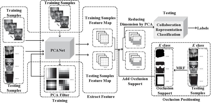
Figure 1 This article main work flow chart.
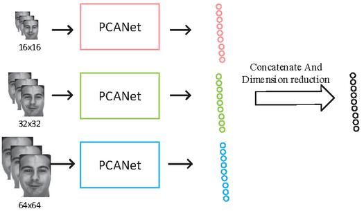
Figure 2 Multi-Scale PCANet.
3.3 The Cooperative Representation Combining PCANet/MS-PCANet with Occlusion Positioning
3.3.1 Modeling
Set as the training sample set, where is the original characteristic dimension of the training sample, and is the number of training samples. The model of this paper is as follows:
| (7) |
where is the testing sample. is an occlusion support array of the same size as the original sample image. Element 1 in means occlusion at the corresponding position of the sample image, and element 1 means no occlusion. “” is the generalized AND operation, indicating that the value of the element corresponding to in the feature graph is set to 0. represents hash coded operator.
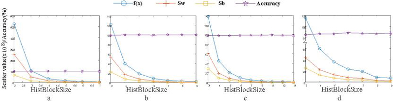
Figure 3 The scatter value and recognition rate of the training set vary with the size of the second partition block (PCA filter sizes from Fig 3a to Fig 3d are respectively , , and , and the horizontal axis HistBlockSize in the figure represents the size of the second partition block).
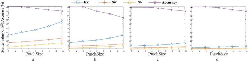
Figure 4 The scatter value and recognition rate of the training set vary with the size of PCA filter (sizes of the second partition block from Fig 4a to Fig 4d are respectively , , and ).
3.3.2 Optimization
For the optimization of the above multi-objective optimization model, this paper adopts the strategy of distributed optimization [8, 1]. When you solve for , you fix , and vice versa.
Step 1: With fixed, the occlusion support was solved by alternately updating and reconstruction error . For the update of , we adopt Markov Random Field algorithm. It is assumed that the normalized training sample set is , and is the test sample. Firstly, the occlusion support is initialized as the column vector , that is, there is no occlusion marker in the occlusion support in the initial state. Repeat the following operations until the maximum number of iterations is reached or stop when for two consecutive iterations is not updated. The occlusion in the training sample set and the test sample is removed to obtain and respectively, and then the reconstruction error is updated:
| (8) |
The error can be updated to , and then the occlusion support can be updated by Markov Random Field:
| (9) |
where is the iteration result of occlusion support. and are respectively the set of edges and nodes in the pixel neighborhood located at in . is the logarithm likelihood function [20] of a given error support. See algorithm 1 for the detailed solution process of occlusion support .
Step 2: Fix and update the decoding coefficient , at which point in the model is known. Therefore, the optimization objective function can be simplified as:
| (10) |
Obviously, the objective optimization function of Equation (10) is a differentiable convex function. According to the occlusion support obtained in the previous step, the pixel corresponding to the position with occlusion marker in in the feature graph and is set to 0, and then the feature graph with occlusion feature removed is coded by hash coding operator . Finally, the least square method can be used to solve:
| (13) | |
| (14) |
Step 3: Repeat steps 1 and 2 until you have a convergent .
3.4 Classification Approach
After the regression factor is obtained, the test sample is reconstructed by the regression factor of various other subspace, and the category of the subspace with the minimum reconstruction error is the category of the test sample. That is,
| (15) |
where is the label of the sample .
4 Experiment and Simulation
4.1 PCA Filter Size Selection
In the process of feature extraction, PCANet network needs to be partitioned twice. The first partitioning is for training PCA filter, and the second partitioning is for hash coding.
As shown in the Figure 3, it can be seen that when the size of the PCA filter is fixed, the size of the second partition block has little impact on the recognition rate and the scatter value (including intra-class scatter , inter-class scatter , difference between intra-class and inter-class divergence, i.e. ) of the training set. Therefore, we do not consider the size of the second block, but only discuss the influence of the size of PCA filter on the dispersion and recognition rate of the training set. Through the optimization Eq. (5), the optimal PCA filter size can be obtained as . However, it can be seen from the Figure 4 that, compared with the filter, the divergence and recognition rate of PCA filter are almost the same, while the efficiency of the algorithm is improved. Therefore, we set the size of the PCA filter to .
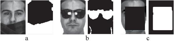
Figure 5 The iterative process of occlusion support for different types of occlusion.
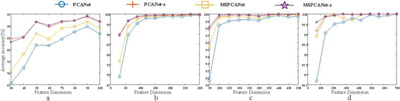
Figure 6 The average recognition rate of different feature dimensions under the same sample quantity (Fig corresponds to 100, 300, 500 and 700 training samples respectively).
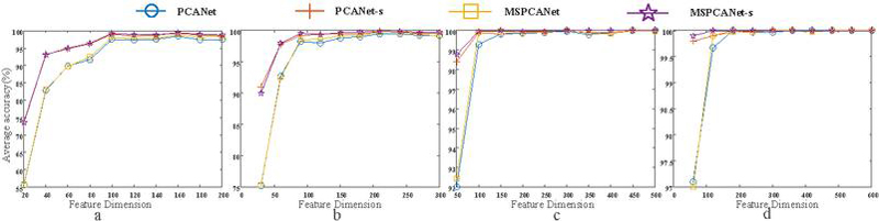
Figure 7 The average recognition rate of different feature dimensions under the same sample quantity (Fig corresponds to 200, 300, 500 and 600 training samples respectively).
4.2 Determination of Occlusion Support
As shown in the Figure 5, Figure. 5a, 5b and 5c respectively show the samples of three occlusion types and their corresponding occlusion supports (a is scarf occlusion, b is sunglasses occlusion and c is block occlusion). It can be seen that the method in this paper can accurately detect the occlusion of scarf and black square, while the shade of sunglasses has a slightly higher false detection rate.
4.3 Non-cooperative Face Recognition on Several Datasets
4.3.1 AR dataset
AR data set [10] is composed of more than 4,000 samples from 126 objects. A maximum of 700 samples with no occlusion were used for training, and 300 samples with scarf occlusion were used for testing. The training samples and test samples are shown in the Figure 8a and 8b. A total of 4 groups of experiments were conducted. The first group(PCANet) adopted all the feature information; the second group(PCANet-s) removed the feature information corresponding to the occlusion (i.e., the occlusion support was added); the third group(MSPCANet) added multi-scale information on the basis of all the features; the fourth group(MSPCANet-s) added multi-scale information on the basis of removing the feature information corresponding to the occlusion. The number of training samples for each group of experiments increased from 1 training sample for each type of object (a total of 100 training samples) to 7 training samples for each type of object (a total of 700 training samples). Under the same training sample number, the average recognition rate of different feature dimensions was tested. As can be seen from the Figure 6, with the increase of training samples, the differences between the results of the four groups became smaller and smaller. However, in the case of a small number of training samples, the recognition effect with occlusion support is obviously better than that without occlusion support, which fully indicates that the expression ability of features can be improved after the occlusion location is known and the occlusion is removed. Without occlusion support, the recognition effect with multi-scale information is slightly better than that with single scale feature information. Of course, adding occlusion support on the basis of multi-scale feature information can still further improve the recognition effect.
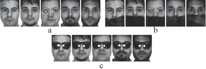
Figure 8 The AR dataset sample(Fig 6a shows the training samples, 6b shows the testing sample with scarf, 6c shows the testing sample with sunglasses.)
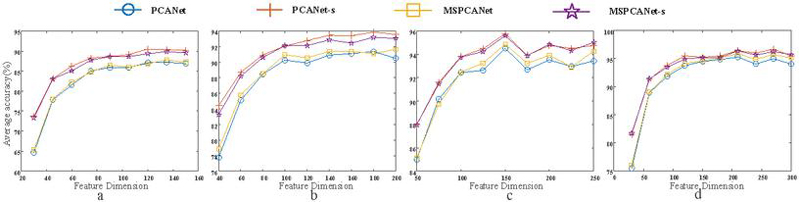
Figure 9 The average recognition rate of different feature dimensions under the same sample quantity (Fig corresponds to 150, 200, 250 and 300 training samples respectively).
In the same experimental setting, the scarf occlusion in the test sample was replaced with sunglasses occlusion, and the testing samples are shown in the Figure 8c.
As shown in Figure 7, with the increase of training samples and the increase of characteristic dimensions, the results of the four groups of experiments showed smaller and smaller differences. And in the case of fewer training samples and smaller characteristic dimensions, the recognition effect with occlusion support is significantly better than that without occlusion support in the experimental group. As is shown in Table 1 and Table 2, the maximum average recognition rate and its variance under each training sample number are listed. We can see that MSPCANet-s has always better performance in the case of small sample.
Table 1 The highest average recognition rate (%) and its variance () vary with the training sample quantity (the feature dimension corresponding to the highest average recognition rate is shown in brackets)
| Method | 100 samples | 300 samples | 500 samples | 700 samples |
| PCANet | 89.735.20(90) | 99.500.023(300) | 99.800.005(400) | 100.00.000(700) |
| PCANet-s | 93.801.90(90) | 99.900.005(270) | 99.970.001(400) | 100.00.000(280) |
| MSPCANet | 91.703.40(90) | 99.700.018(300) | 99.930.002(500) | 100.00.000(490) |
| MSPCANet-s | 94.232.10(90) | 99.900.005(270) | 100.00.000(400) | 100.00.000(280) |
Table 2 The highest average recognition rate (%) and its variance () vary with the training sample quantity (the feature dimension corresponding to the highest average recognition rate is shown in brackets)
| Method | 200 samples | 300 samples | 500 samples | 600 samples |
| PCANet | 98.435.20(160) | 99.470.128(210) | 100.00.000(450) | 100.00.000(180) |
| PCANet-s | 99.271.90(160) | 99.770.050(210) | 100.00.000(300) | 100.00.000(180) |
| MSPCANet | 98.903.40(160) | 99.770.099(240) | 100.00.000(300) | 100.00.000(300) |
| MSPCANet-s | 99.472.10(160) | 99.900.035(210) | 100.00.000(150) | 100.00.000(120) |
Table 3 The highest average recognition rate (%) and its variance () vary with the training sample quantity (the feature dimension corresponding to the highest average recognition rate is shown in brackets)
| Method | 150 training samples | 200 training samples | 250 training samples | 300 training samples |
| 350 testing samples | 300 testing samples | 250 testing samples | 200 testing samples | |
| PCANet | 87.200.30(135) | 91.370.69(180) | 94.520.48(150) | 95.300.36(210) |
| PCANet-s | 90.490.23(120) | 93.870.22(180) | 95.760.93(150) | 96.700.26(270) |
| MSPCANet | 87.770.50(135) | 91.670.11(200) | 94.880.20(150) | 95.900.30(210) |
| MSPCANet-s | 89.860.59(135) | 93.200.31(180) | 95.600.32(150) | 96.400.16(210) |
It can be seen that the effect of occlusion position information added is obviously better than that without occlusion position information, whether it is shaded by sunglasses or scarves.
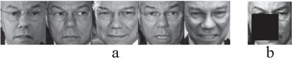
Figure 10 The LFW dataset sample(Fig 10a shows the training samples, 10b shows the testing sample with block occlusion.)
4.3.2 LFW dataset
LFW [7] is a face data set collected in an unconstrained environment. In the experiment, we adopted the corrected LFW3D-SDM database based on SDM feature point detection method. The training samples and the testing samples are shown in the Figure 10. It can be seen that even after correction, the image samples of the same object still have uneven illumination and difference of expression changes, which makes the experiment still challenging. To verify the performance of this method will changes with the change of the training sample, each object in turn select 3, 4, 5, and 6 samples used for training and use the rest 7, 6, 5 and 4 samples of each object for testing. And all the testing samples add occlusion that is 0.4 times the size of the image sample. As shown in Figure 9, it can be seen that, similar to the results on the AR data set, the classification effect is obviously better by adding the occlusion position information than by not adding the occlusion position information. In the LFW data set, from low-dimensional features to high-dimensional features, the classification effect of adding occlusion location information is better than that of no occlusion location information. This is because the sample images in the LFW data set still have great differences in places beyond occlusion. And the higher the feature dimension to preserve the more information, so the higher the feature dimension is, the more prominent the role of occlusion location information will be. Moreover, the classification performance was improved with the increase of the number of training samples whether or not the occlusion location information was added. Also in the Table 3, the highest average recognition rate and variance, varying with different training sample numbers, are given. It can also be seen that the effect of occlusion location information added is obviously better than that without.
Finally, in order to evaluate the overall performance of several methods, Their ROC curves are given in Figure 11. It can be seen that the ROC curves of MSPCANet-s and PCANet-s with occlusion location information are closer to the upper left corner of the coordinate system, indicating better performance.
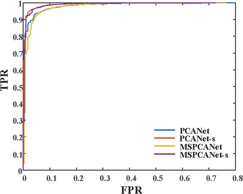
Figure 11 ROC curve.
5 Conclusion
In the test of non-cooperative face recognition, the performance of the classifier will be reduced due to the occlusion in the test sample. To solve this common problem, we first use Markov random fields to locate occlusion in test samples. Then, the feature information corresponding to the occlusion in the feature map is removed, so as to eliminate the influence of occlusion in the classification process. Moreover, this paper proposes a quantifiable method to select the filter size, that is, to determine the filter size according to the degree of clustering among the characteristic representations of each sample. The experimental results show that the performance of the collaborative representation model is improved by integrating multi-scale feature information and adding occlusion location information in different databases.
Acknowledgments
This study is supported by Jiangsu Engineering Research Center of Digital Twinning Technology for Key Equipment in Petrochemical Process (No. DT2020720).
References
[1] Esther Bonacker. Perturbed Projection Methods in Convex Optimization – Applied to Radiotherapy Planning. PhD thesis, Kaiserslautern University of Technology, Germany, 2020.
[2] Sijia Cai, Wangmeng Zuo, Lei Zhang, Xiangchu Feng, and Ping Wang. Support vector guided dictionary learning. In David J. Fleet, Tomás Pajdla, Bernt Schiele, and Tinne Tuytelaars, editors, Computer Vision – ECCV 2014 – 13th European Conference, Zurich, Switzerland, September 6–12, 2014, Proceedings, Part IV, volume 8692 of Lecture Notes in Computer Science, pages 624–639. Springer, 2014.
[3] Tsung-Han Chan, Kui Jia, Shenghua Gao, Jiwen Lu, Zinan Zeng, and Yi Ma. Pcanet: A simple deep learning baseline for image classification? IEEE Trans. Image Process., 24(12):5017–5032, 2015.
[4] Jie Chen, Shiguang Shan, Chu He, Guoying Zhao, Matti Pietikäinen, Xilin Chen, and Wen Gao. WLD: A robust local image descriptor. IEEE Trans. Pattern Anal. Mach. Intell., 32(9):1705–1720, 2010.
[5] Hongmei Chi, Haifeng Xia, Lifang Zhang, Chunjiang Zhang, and Xin Tang. Competitive and collaborative representation for classification. Pattern Recognition Letters, 132:46–55, 2020.
[6] Hazim Kemal Ekenel and Rainer Stiefelhagen. Why is facial occlusion a challenging problem? In Massimo Tistarelli and Mark S. Nixon, editors, Advances in Biometrics, Third International Conference, ICB 2009, Alghero, Italy, June 2–5, 2009. Proceedings, volume 5558 of Lecture Notes in Computer Science, pages 299–308. Springer, 2009.
[7] Gary B. Huang, Marwan Mattar, Tamara Berg, and Erik Learned-Miller. Labeled faces in the wild: a database for studying face recognition in unconstrained environments.
[8] Antoine Lesage-Landry, Iman Shames, and Joshua A. Taylor. Predictive online convex optimization. Autom., 113:108771, 2020.
[9] Xiaoxin Li and Ronghua Liang. A review for face recognition with occlusion: From subspace regression to deep learning. Chinese Journal of Computers, 041(001):177–207, 2018.
[10] AM Martinez and R Benavente. The ar face database.
[11] Yi Sun, Xiaogang Wang, and Xiaoou Tang. Deeply learned face representations are sparse, selective, and robust. In IEEE Conference on Computer Vision and Pattern Recognition, CVPR 2015, Boston, MA, USA, June 7–12, 2015, pages 2892–2900. IEEE Computer Society, 2015.
[12] Xingjie Wei, Chang-Tsun Li, and Yongjian Hu. Robust face recognition under varying illumination and occlusion considering structured sparsity. In 2012 International Conference on Digital Image Computing Techniques and Applications, DICTA 2012, Fremantle, Australia, December 3–5, 2012, pages 1–7. IEEE, 2012.
[13] John Wright, Allen Y. Yang, Arvind Ganesh, Shankar S. Sastry, and Yi Ma. Robust face recognition via sparse representation. IEEE Trans. Pattern Anal. Mach. Intell., 31(2):210–227, 2009.
[14] Huosheng Xie, Yafeng Zhang, and Zesen Wu. Fabric defect detection method combing image pyramid and direction template. IEEE Access, 7:182320–182334, 2019.
[15] Meng Yang and Lei Zhang. Gabor feature based sparse representation for face recognition with gabor occlusion dictionary. In Kostas Daniilidis, Petros Maragos, and Nikos Paragios, editors, Computer Vision – ECCV 2010 – 11th European Conference on Computer Vision, Heraklion, Crete, Greece, September 5–11, 2010, Proceedings, Part VI, volume 6316 of Lecture Notes in Computer Science, pages 448–461. Springer, 2010.
[16] Meng Yang, Lei Zhang, Xiangchu Feng, and David Zhang. Fisher discrimination dictionary learning for sparse representation. In Dimitris N. Metaxas, Long Quan, Alberto Sanfeliu, and Luc Van Gool, editors, IEEE International Conference on Computer Vision, ICCV 2011, Barcelona, Spain, November 6–13, 2011, pages 543–550. IEEE Computer Society, 2011.
[17] Meng Yang, Lei Zhang, Simon Chi-Keung Shiu, and David Zhang. Robust kernel representation with statistical local features for face recognition. IEEE Trans. Neural Networks Learn. Syst., 24(6):900–912, 2013.
[18] Meng Yang, Lei Zhang, Jian Yang, and David Zhang. Metaface learning for sparse representation based face recognition. In Proceedings of the International Conference on Image Processing, ICIP 2010, September 26-29, Hong Kong, China, pages 1601–1604. IEEE, 2010.
[19] Lei Zhang, Meng Yang, and Xiangchu Feng. Sparse representation or collaborative representation: Which helps face recognition? In Dimitris N. Metaxas, Long Quan, Alberto Sanfeliu, and Luc Van Gool, editors, IEEE International Conference on Computer Vision, ICCV 2011, Barcelona, Spain, November 6–13, 2011, pages 471–478. IEEE Computer Society, 2011.
[20] Zihan Zhou, Andrew Wagner, Hossein Mobahi, John Wright, and Yi Ma. Face recognition with contiguous occlusion using markov random fields. In IEEE 12th International Conference on Computer Vision, ICCV 2009, Kyoto, Japan, September 27–October 4, 2009, pages 1050–1057. IEEE Computer Society, 2009.
Biographies

Zhi Zhang Hefei Institutes of Physical Science, Chinese Academy of Sciences, Hefei 230031, Anhui, China.

Bingyu Sun Hefei Institutes of Physical Science, Chinese Academy of Sciences, Hefei 230031, Anhui, China.
Journal of Web Engineering, Vol. 25_1, 33–50
doi: 10.13052/jwe1540-9589.2513
© 2026 River Publishers