Towards Real-time Underwater Object Detection and Identification: Integrating Acoustic Sensing with Edge Computing
Shekhar Tyagi∗, Akshat Shah and Abhishek Srivastava
Department of Computer Science and Engineering, Indian Institute of Technology, Indore, India
E-mail: shekhartyagicse@gmail.com; akshats1607@gmail.com; asrivastava@iiti.ac.in
∗ Corresponding Author
Received 23 September 2025; Accepted 15 December 2025
Abstract
In this work, we present a method to streamline underwater object detection, environmental monitoring, and surveillance. The proposed system employs an underwater acoustic sensor (UAS) network to detect and analyses objects within a three-dimensional underwater space, considering constraints imposed by acoustic path loss. The approach combines three key techniques–Delaunay’s convex hull-based reconstruction, the laws of magnetic equilibrium, and the Doppler effect–to improve the identification of object type, shape, location, and motion. Sensors are arranged in an optimized grid, with each grid containing eight sensors and a central insulated magnetometer to measure net magnetic field intensity. Data collected by the sensors is transmitted to a surface anchor or sink node for further processing and analysis. A prototypical deployment in an artificial pond further validates our approach, using a waterproof ultrasonic sensor, an electromagnetic coil, and a magnetometer synchronized via Arduino Uno. Real-time measurements confirm accurate detection and tracking of objects, demonstrating the effectiveness and feasibility of the proposed edge-enabled underwater monitoring framework.
Keywords: Underwater acoustic sensor network, sensor deployment, underwater object detection, underwater object identification.
1 Introduction
Underwater environmental monitoring plays a critical role in diverse domains such as biodiversity conservation, defense, resource prospecting, and infrastructure evaluation [1, 2]. Given the impacts of climate change and the deterioration of marine ecosystems, underwater monitoring has become increasingly important. Underwater acoustic sensor (UAS) networks are a widely adopted approach for such monitoring [3]. The present work builds upon and extends our study [4], and includes a prototypical deployment to evaluate and validate the proposed methodology.
Investigating and monitoring underwater environments is challenging [5] due to poor visibility and signal attenuation. Traditional technologies such as sonar, imaging systems, and ROVs/AUVs (remotely operated vehicles/autonomous underwater vehicles) also have inherent limitations [6]. Sonar is efficient over larger distances but is affected by interference, whereas imaging requires good lighting and is often too expensive. ROVs and AUVs are efficient, but they use a lot of energy and equipment setups. Current underwater object detection methods provide a strong foundation in UAS networks but most of them are dependent on machine learning (CNN [7], YOLO [8]) and computer vision (OpenCV) [9], which require better visibility conditions, lack bathymetric analysis and fail to address path losses. Their accuracy is limited and are only feasible in regions with good visibility.
For instance, Fossum et al. [10] and Fayaz et al. [11] used CNN and YOLO (you only look once)-based techniques for underwater tracking. However, these methods rely heavily on visual datasets and show limited effectiveness ( accuracy) in underwater conditions with high depth and low visibility. Furthermore, they do not account for acoustic path loss, which is essential for accurate underwater detection. Similarly, Hayat et al. [12] and Zhang et al. [13] investigated underwater object detection using OpenCV and YOLO-based approaches, which also demonstrated limited accuracy ().
The proposed approach addresses these challenges as follows:
1. It begins with bathymetric analysis and applies acoustic path loss models to deploy the sensors accurately at optimal locations.
2. The object detection phase integrates Delaunay’s convex hull-based point cloud reconstruction [14], the law of magnetic equilibrium [15], and the Doppler effect [16] to enhance the accurate identification of object type (living or non-living), shape, location, and state (stationary or in motion).
3. The sensor-collected data is transmitted to a surface anchor or sink node, enabling real-time processing and analysis.
The remainder of this paper is organized as follows: Section 2 presents the background work; Section 3 details the proposed methodology; Section 4 describes the experiments and results, validating the effectiveness of the approach through comparisons with existing methods and real-world deployment; Section 5 discusses the prototypical setup; and Section 6 concludes the paper.
2 Background Work
This section provides an overview of key underwater object detection methods, highlighting their contributions, limitations, and type (machine learning or computer vision). Traditional approaches, such as imaging, sonar, and robotic vehicles like ROVs and AUVs, often struggle in low-visibility conditions, deep-water environments, and areas with weak signals.
Several methods have been explored, mainly categorized as machine learning-based and computer vision-based techniques. Table 1 summarizes their type, key features, limitations, and reported accuracy.
Table 1 Comparison of existing underwater object detection approaches
| Approach | Type | Technique/dataset | Limitations | Accuracy |
| Fossum et al. [10] | ML-based | CNN, visual datasets | Poor performance in low visibility, limited depth, ignores path loss | 75% |
| Fayaz et al. [11] | ML-based | YOLO CNN, visual datasets | Same as above, <75% accuracy, limited deep-sea application | <75% |
| Hayat et al. [12] | CV-based | OpenCV, imaging datasets | Ineffective in low visibility, no bathymetric or path loss integration, not real-time | Low |
| Zhang et al. [13] | CV-based | OpenCV YOLO, imaging datasets | Limited by visibility, no bathymetric/path loss modeling, real-time only | 76.8% |
2.1 Machine Learning-based Approaches
Fossum et al. [10] and Fayaz et al. [11] applied deep learning techniques such as CNN and YOLO for underwater imaging and video-based object detection. These methods rely heavily on visual datasets, reducing effectiveness in low-visibility underwater conditions. They also ignore acoustic path loss, which is important for accurate underwater detection. Accuracy is moderate, with Fossum et al. reporting 75% and Fayaz et al. below 75%.
2.2 Computer Vision-based Approaches
Hayat et al. [12] and Zhang et al. [13] used OpenCV-based techniques, with Zhang et al. additionally employing YOLO. These approaches also depend on imaging datasets, limiting their performance in low-visibility areas. Neither incorporates bathymetric analysis or acoustic path loss modeling, although Zhang et al. supports real-time monitoring. Accuracy remains limited, with Zhang et al. achieving 76.8% and Hayat et al. lower.
The existing underwater object detection methods suffer from several limitations, including heavy reliance on visual or imaging datasets, which reduces performance in low-visibility environments, lack of bathymetric analysis and path loss modeling, limited applicability in deep-water or complex settings, and moderate accuracy with high computational complexity. The proposed approach addresses these shortcomings by removing dependence on visual datasets, incorporating bathymetric analysis and acoustic path loss models, and combining acoustic-based sensing with Delaunay’s convex hull-based reconstruction, the law of magnetic equilibrium, and the Doppler effect. As a result, it provides a robust, scalable, real-time, and accurate system suitable for complex underwater environments.
3 Proposed Methodology
This section describes the step-by-step approach to detecting and analyzing objects present underwater using the proposed sensor system.
3.1 Extraction of RoI and Topography Analysis
As illustrated in Figure 1a, the approach begins with selecting the region of interest (RoI) using Google Earth tools [17], where coordinate points are carefully placed and exported as a KML (keyhole markup language) file. This file contains the latitude and longitude of each point of interest. Depth information for these points is then obtained using an advanced converter API [18]. The values thus obtained are stored in a CSV (comma separated values) file. Finally, the data in the CSV file is plotted as a bathymetric distribution using a specialized tool named QuickGrid [19], showing depths, which helps in further calculations required for topography analysis, as illustrated in Figure 1b.
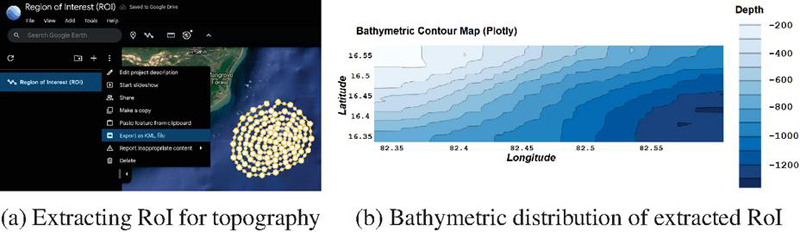
Figure 1 Extracted RoI and its bathymetric distribution.
The bathymetric map enables the evaluation of the locations of the detected objects with good accuracy. The UAS system is able to determine whether an object is resting on the seabed or suspended in the water based on its location. They can also be used for varied tasks such as identification of stationary debris/wreckage, tracking underwater vehicles or aquatic organisms, tracking suspicious underwater activities and so on.
3.2 Path Loss Calculations for Underwater Environments
Acoustic propagation is widely used for underwater monitoring, but it has several notable limitations, including absorption and transmission losses [20]. These are due largely to factors like frequency, pH, temperature, salinity, turbidity, depth and flow of waves and tides. In UAS networks, attenuation is significantly affected by these losses and leads to reduction of intensity of sound as it travels through water.
Absorption loss refers to the loss of acoustic energy as sound waves move through water. This energy is turned into heat due to the properties of the water and the frequency of the sound wave. Larger the frequency of sound, greater the absorption loss.
Transmission loss on the other hand is the total loss of acoustic energy in the medium. This loss occurs due to the spread of wave and absorption losses. Greater the distance between the source and the receiver, the higher is the transmission loss.
The Anslei–McColm acoustic path loss model [21] provides mechanisms to compute how sound waves behave underwater. It computes that sound absorption increase with acidity (pH decreasing) and decreases with higher salinity at lower frequencies. Temperature generally reduces absorption, except near specific relaxation frequencies and for boric acid and for magnesium sulfate, where absorption increases. Whereas, at greater depths, high-frequency absorption decreases, but waves increase both absorption and transmission losses. This model calculates relaxation frequencies and using the following equations:
| (1) | |
| (2) |
where is the salinity of water in parts per thousand (ppt), and is the temperature of water in degrees Celsius ().
Based on the calculated relaxation frequencies, the absorption coefficient can be calculated using [21]:
| (3) |
where is the absorption coefficient (in dB/km), is the depth (in km), and is the frequency of acoustic signals (in kHz).
Further transmission loss can be calculated using:
| (4) |
where is the transmission loss (in dB), is the propagation range (in km), and is the absorption coefficient (in dB/km).
These loss calculations are necessary to determine the new propagation ranges due to the changed behaviour of the sensors and acoustic signals in the real-time underwater environment which may also require to modify the grid arrangement.
3.3 System Arrangement for Object Identification
In this section, we will discuss underlying sensor modifications and the deployment strategy.
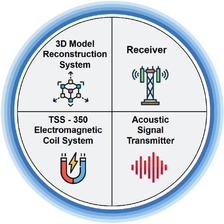
Figure 2 Components of the sensor.
3.3.1 Components of UAS modification
Figure 2 shows the construction of the UAS. The sensor has been modified and equipped with four components and are described as follows:
1. Reconstruction system: The sensors produce sound waves, which pass through water and hit the surface of the object and then return to the sensor. Based on the velocity of acoustic signals underwater and the time taken by the sound waves to collide with the object and return (as calculated by the receiver itself), the system determines the distance from the sensor to the point of reflection on the object’s surface. Finally, using the known coordinates of the sensor’s location (), the distance between the sensor and the point of reflection and the unit vector along that direction, the coordinates of that point () are calculated. This is applicable to computing coordinates of several points on the object’s surface from where the acoustic signals are reflected. Mathematically define as follows:
| (5) | |
| (6) | |
| (7) | |
| (8) |
where
• ; ; ,
• : Distance between th sensor and th point of reflection (in m),
• : Velocity of sound in water, i.e. 344 m/s,
• : Time taken by acoustic signal to travel (in seconds).
• (): Coordinates of th sensor,
• (): Coordinates of th point of reflection,
• : Unit vector in direction of reflected signal.
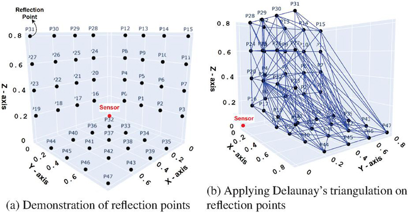
Figure 3 Visualization of reflection points and Delaunay triangulation.
After computing the reflection points, a point cloud is formed on the object’s surface within the sensor’s range. Delaunay’s triangulation then connects these points, creating an optimal and stable structure. Figure 3a depicts the 3D region with reflection points, while Figure 3b illustrates the Delaunay triangulation process [14]. Note that the dimensions are in meters.
1. A set of reflection points P(), where is the number of reflection points, and each has coordinates in 3D space, is obtained from the above process. The convex hull is the smallest convex polygon (or polyhedron in 3D) that contains all the points.
2. Initially, a tetrahedron that contains all the points is constructed. The convex hull helps to determine the boundary of the triangulation. The triangulation starts with an initial set of tetrahedrons. New points are inserted one by one into the triangulation and the tetrahedrons which are already present in the space are updated to include the new point.
3. Multiple tetrahedrons are formed in the space by considering any three points such that no other point lies inside the circumcircle of these three points.
4. The algorithm iteratively keeps on connecting the points and edges and keeps on constructing tetrahedrons that satisfy the above property until it is ensured that no such set of three points is left in which the condition of Delaunay’s triangulation is satisfied.
Finally, a mesh is obtained where the minimum angles are maximized with iterations. By applying this method, a 3D mesh is obtained which shows the geometry of a part of the object. By collectively analyzing results of all the sensors, a strong perception of the shape and size of the object is obtained.
2. Receiver: The first task of the receiver component is to measure the frequency of the signal echoed or reflected from the object. This frequency may be less than or equal to the original frequency of the signal emitted from the sensor. This can be confirmed using the Doppler effect [22], which is a fundamental principle in physics. It describes the change in frequency of wave (sound or light) due to the relative motion between source and the object. In contrast to this, if the receiver detects change in frequency and assuming the source at rest, the velocity of the object can be determined using the Doppler effect. The formulation is shown below:
| (9) |
where is the velocity of the object with respect to the source (in m/s), and is the frequency received by the receiver (in kHz).
The second task of the receiver is to figure out the time of flight and the direction of the emitted signal using the direction of the reflected signal. The receiver senses the reflected signal and then calculates unit vector along that direction. This information is shared with the reconstruction system that is required to calculate the locations of points of reflection.
3. Electromagnetic coil system (ECS): This uses a magnet (electromagnet) that creates a magnetic field with the help of electric current. The TSS-350 ECS [23] is used here over permanent magnets as its magnetic strength can be dynamically controlled by changing the electric current. An ECS is present within each of the sensors and produces a strong and steady magnetic field surrounding the corresponding sensor. The magnetometer will measure the magnetic field at equilibrium. As soon as an underwater object enters the region common to the sensor’s range and the magnetic field, equilibrium is disturbed and fluctuations are observed in the magnetometer reading. These fluctuations will provide a perception of the object that it is not a living organism but a ferromagnetic object. This is because the magnetic field does not change drastically by intervention from weakly or non-ferromagnetic materials. It is mathematically represented as follows:
| (10) |
where is the magnetic flux density (in Tesla), is the permeability of free space H/m), is the magnetic field intensity (in Tesla), and is the magnetization (in A/m).
There are three types of magnetic materials: paramagnetic, diamagnetic and ferromagnetic. Paramagnetic materials are those which have attraction towards magnets. Diamagnetic materials are those which suffer repulsion from magnets. Ferromagnetic substances are those which not only show high attraction towards magnets but also retain the magnetic property.
The magnetic susceptibility () and its magnitude affects the magnetic strength of a substance. Weakly diamagnetic materials have negative with a lower magnitude, whereas strongly diamagnetic materials have negative with a higher magnitude. Similarly, weakly paramagnetic materials have small positive and strongly paramagnetic materials have high positive . Ferromagnetic materials are similar to strongly paramagnetic materials but can also retain magnetic properties. Most elements in the periodic table are diamagnetic. Table 2 can be referred to for further details on the magnetic behavior of elements [24].
Table 2 Magnetic properties of selected materials
| Material | [10-5] (SI units) | Type |
| Aluminium | 2.2 | Paramagnetic |
| Caesium | 5.1 | Paramagnetic |
| Lithium | 1.4 | Paramagnetic |
| Magnesium | 1.2 | Paramagnetic |
| Sodium | 0.72 | Paramagnetic |
| Tungsten | 6.8 | Paramagnetic |
| Superconductor | 100000 | Diamagnetic |
| Pyrolytic carbon | 40.9 | Diamagnetic |
| Bismuth | 16.6 | Diamagnetic |
| Neon | 6.74 | Diamagnetic |
| Mercury | 2.9 | Diamagnetic |
| Silver | 2.6 | Diamagnetic |
| Carbon (diamond) | 2.1 | Diamagnetic |
| Lead | 1.8 | Diamagnetic |
| Carbon (graphite) | 1.6 | Diamagnetic |
| Copper | 1 | Diamagnetic |
| Pure iron | 200000 | Ferromagnetic |
| Carbon steel (ship hulls) | 1000–10000 | Ferromagnetic |
| Nickel–iron alloy (permalloy) | 80000–100000 | Ferromagnetic |
| Magnetite (Fe3O4) | 70000 | Ferromagnetic |
| Stainless steel (430 Grade) | 750–1500 | Ferromagnetic |
| Hydroxyl iron composite (cloaking) | 50000–200000 | Ferromagnetic |
Most biological tissues are weakly diamagnetic in nature. This property can be useful for determining whether the object in water is the body of a living organism. Diamagnetic materials have a negative magnetization which is proportional to the magnetic field.
| (11) |
There is also a high chance that paramagnetic materials will be encountered. These may be wreckage or part of some machinery. Paramagnetic materials have a positive magnetization which is proportional to the magnetic field.
| (12) |
Using (10), (11) and (12), we get,
| (13) | |
| (14) |
For very small values of , becomes very small which implies that there is negligible effect on magnetic field intensity caused by the object and thus, .
4. Acoustic signal transmitter: The acoustic signal transmission is by default set to a spherical mode of propagation. These signals are transmitted in the form of concentric spheres outwards the sensor.
3.3.2 Deployment strategy for UASs
Figure 4 represents the deployment strategy of the sensors using the proposed approach. The sensors are deployed within a uniform grid, each grid consisting of 8 sensors. Each sensor is equipped with the modifications as discussed above. In the center lies a magnetometer to measure the overall magnetic field equilibrium within the grid.
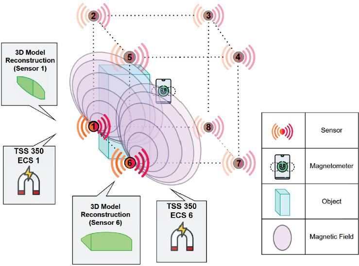
Figure 4 Deployment architecture.
3.3.3 Time complexity analysis
The complexity of entire process is contributed by the four main components.
1. The reading of the magnetic field fluctuations through the magnetometer can be understood as a constant time complexity of .
2. The process of determining object motion through the Doppler Effect also has a constant time complexity of as it involves direct mathematical computation of object’s velocity.
3. The process of calculating all the reflection points involves first calculating the time of flight of the number of signals emitted with complexity of (for being number of signals emitted). The signals reaching back after collision from the object have complexity of (for being number of signals returned) making the total . Moreover, the time complexity to compute X,Y and Z coordinates for each reflection point is (for being the number of reflection points). Adding all of them simplifies to linear time complexity of .
4. Finally the process of Delaunay triangulation has the most optimal time complexity of (for being the number of reflection points in the point cloud).
3.3.4 Time estimation model and accuracy analysis
The total time taken by the grid to process an object is given by:
| (15) |
where
• : Time required to analyze magnetometer fluctuations and determine whether the object is living or nonliving.
• : Time needed to process Doppler effect data and determine the object’s motion.
• : Time required to calculate points of reflection from the object’s surface using acoustic signals.
• : Fixed time for constructing a 3D representation of the object from sensor data.
The analysis of the accuracy of the reconstruction system is significant throughout the process. It is important to note that the accuracy can be calculated by dividing the number of points in the point cloud that participate in the Delaunay triangulation by the total number of points in the point cloud, as shown in Equation 16.
| (16) |
However, there may be some points present on the boundary of the part of object in the sensor range. This can have a negative but negligible effect on the overall accuracy and the perception accuracy still stays 100% as it depends on the clarity of the shape of the object which is still understandable.
Algorithm 1 Underwater object detection and analysis.
1: RoI coordinates from Google Earth, Sensor Data
2: Detected and analyzed objects
3: Step 1: Extract RoI
4: Select RoI by manually placing coordinate points
5: Export RoI as KML file
6: Extract latitude, longitude and maximum elevation
7: Step 2: Create bathymetric map
8: Parse KML file for coordinate points
9: Fetch depth values using API
10: Store extracted data in CSV format
11: Generate 3D bathymetric distribution
12: Step 3: Compute path loss
13: for each sensor location do
14:Compute relaxation frequencies and using:
15:
16:
17:Compute absorption coefficient :
18:
19:Compute transmission loss:
20:
21: end for
22: Step 4: Object detection
23: for each acoustic signal received do
24:Compute time of flight (TOF)
25:Determine reflection point
26:Identify object type and position
27:Calibrate Doppler and magnetometer sensors
28:Evaluate object location
29:Output final object detection results
30: end for
4 Results and Evaluation
In this section we will compare the outcomes of our approach with several other existing methods based on some key parameters.
4.1 Simulation Environment
We have developed a simulation environment for this using Python 3.10.11 on a Notebook Computer equipped with an Intel i7 12th-gen processor, 16 GB RAM, and a dedicated NVIDIA graphics card. The simulation process is shown in Figure 5a where a 3D underwater region of m is assumed at a random location. Inside the region an imaginary object is considered using Convex Hull at coordinates .
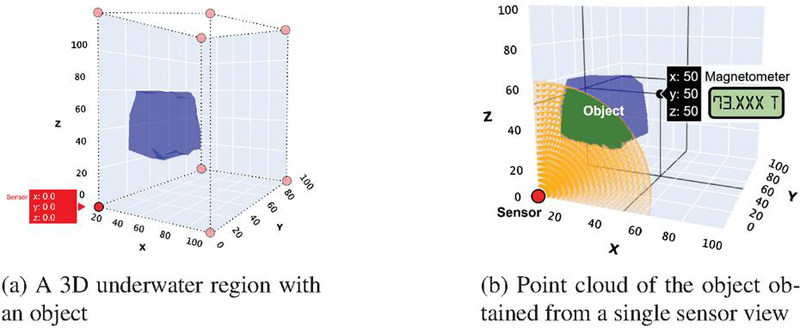
Figure 5 Simulation process.
The sensors are placed at all extreme corners of the grid. However, the sensors’ position may vary a little with consideration of the path loss model. Also, to reduce complexities, further simulations are carried out for a single sensor placed at coordinates . A magnetometer is placed at the center of the grid which measures the equilibrium magnetic field intensity. The readings are shared to the sink node managing the grid.
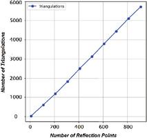
Figure 6 Number of triangulations vs number of reflection points.
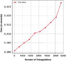
Figure 7 Time taken vs number of triangulations.
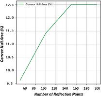
Figure 8 Covered area of Convex Hull vs number of reflection points.
The process begins by determining sensor locations using bathymetry analysis. When an underwater object enters the grid, magnetometer readings may fluctuate due to disturbances in the magnetic field, indicating whether the object is ferromagnetic. The Doppler effect then determines the object’s velocity and helps calculate reflection points of acoustic signals. Based on magnetometer fluctuations and velocity, the object is classified as living, non-living, or machinery. Delaunay’s point cloud triangulation reconstructs the object’s surface within the sensor’s propagation range, with green tetrahedrons filling the point cloud, as shown in Figure 5b. Data from all eight sensors is analyzed collectively for higher perception accuracy and sent to the sink node for transmission to the base station. The total time taken during the simulation process for a single sensor can be calculated using Equation 15. The and depend on the real-world scenarios and cannot be estimated in the simulation. However, they can be assumed as a constant total time of . The time taken to calculate points of reflection from the object’s surface using acoustic signals came out to be 0.1457 seconds. The time for constructing a 3D reconstruction of the object came out to be 4.2935 seconds. Hence, the total time is 0.1457 + 4.2935 = 4.4392 seconds.
Figure 7 represents nearly linear variation of the total number of triangulations as we increase the number of reflection points. Figure 7 represents the time taken to construct final object with different number of triangulations. Figure 8 represents the percentage of area covered for different numbers of reflection points. Figure 9 represents percentage of area covered at reaching different number of simplices. A simplex is a fundamental building block of the triangulation. A 0-simplex is a point, 1-simplex is a line segment connecting two points, 2-simplex a triangle and 3-simplex a tetrahedron and so on. We can also say that -simplex is nothing but the convex hull of points in -dimensional space. During the triangulation process in the point cloud we achieve a number of tetrahedrons which increases the number of simplices.
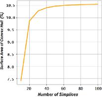
Figure 9 Covered area of Convex Hull vs number of simplices.
4.2 Comparative Analysis with Existing Underwater Object Detection Techniques
In this section, we compare the outcomes of our approach with several existing methods based on key performance parameters. Although a direct comparison is challenging due to variations in experimental setups and results, we have considered several important criteria, including accuracy, depth limit, time complexity, real-time monitoring capability, dependency on datasets, and the use of imaging and videography equipment. The comparative analysis is presented in Table 3.
Table 3 Comparative analysis of the proposed approach with existing methods based on various parameters
| Proposed | Fossum | Fayaz | Hayat | Zhang | |
| Parameter | approach | et al. [10] | et al. [11] | et al. [12] | et al. [13] |
| Imaging/video architecture | None | CNN | CNN, YOLO | OpenCV | OpenCV, YOLO |
| Bathymetric analysis | Yes | No | No | No | No |
| Path loss consideration | Yes | No | No | No | No |
| Real-time monitoring | Yes | Yes | Yes | No | Yes |
| Dataset | None | J-EDI | Heriot-Watt dataset | None | Robot target catching dataset |
| Depth limit | Only pressure constraint | 300 m | Until Visibility | Until Visibility | Until Visibility |
| Time complexity | O() | >O() | O() | O() | O() |
| Accuracy | 100% | 75% | <75% | Low | 76.8% |
5 Prototypical Deployment
Study area: An artificial pond located in Simrol, Indore, Madhya Pradesh, with an approximate area of 4260 square meters, was identified as a suitable site for the deployment of underwater sensor networks. The site offers a naturalistic setting and appropriate hydrological conditions, making it an appropriate and controlled environment for experimental validation of UWSN. Figure 10 represents the RoI of the pond with its entire region covered by the data points plot using Google Earth. Figure 11 represents the 2D and 3D view of the bathymetry of the extracted RoI, created with the help of QuikGrid.
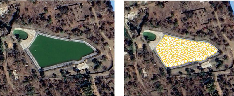
Figure 10 RoI: Simrol pond.
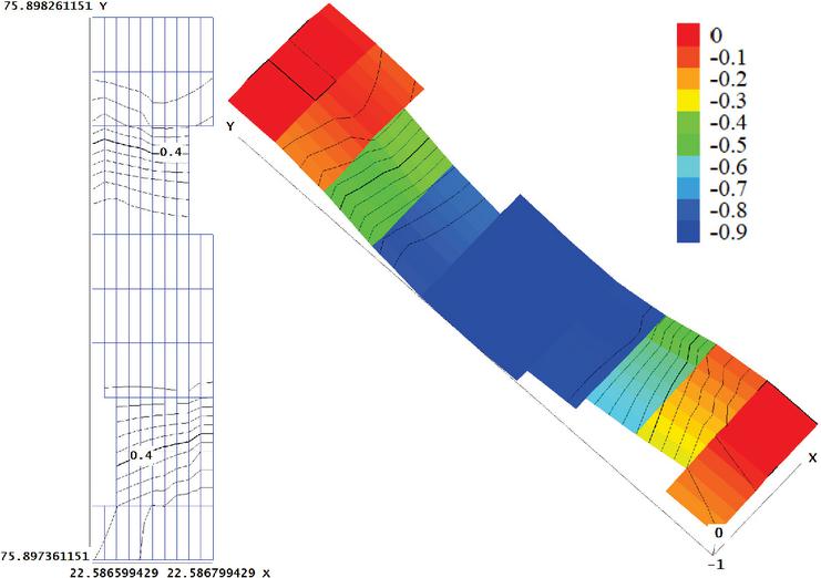
Figure 11 2D and 3D bathymetry of extracted RoI.
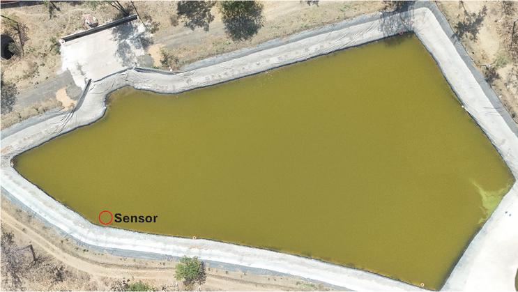
Figure 12 Deployed sensor.
Table 4 Specifications of the ultrasonic sensor
| Parameter | Value |
| Item type | Ultrasonic distance sensor |
| Measurement accuracy | |
| Operating voltage | DC 3.3V–5V |
| Average current | 8 mA |
| Temperature compensation | Yes |
| Range | 3–450 cm |
| Output mode | UART automatic |
The implementation has been done for a single sensor placed at a location as shown in Figure 12. The sensor used is a waterproof ultrasonic sensor with the specifications as listed in Table 4.
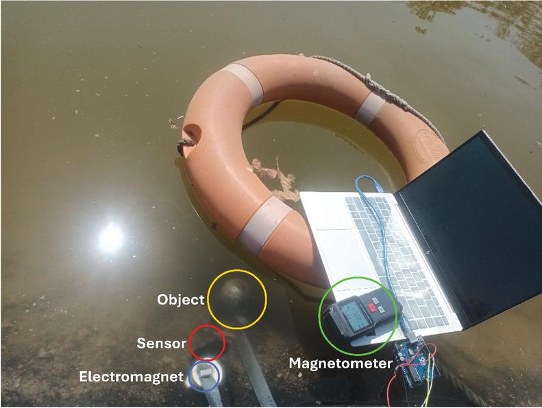
Figure 13 Zoomed in view of the placed sensor along with the object and the connections.
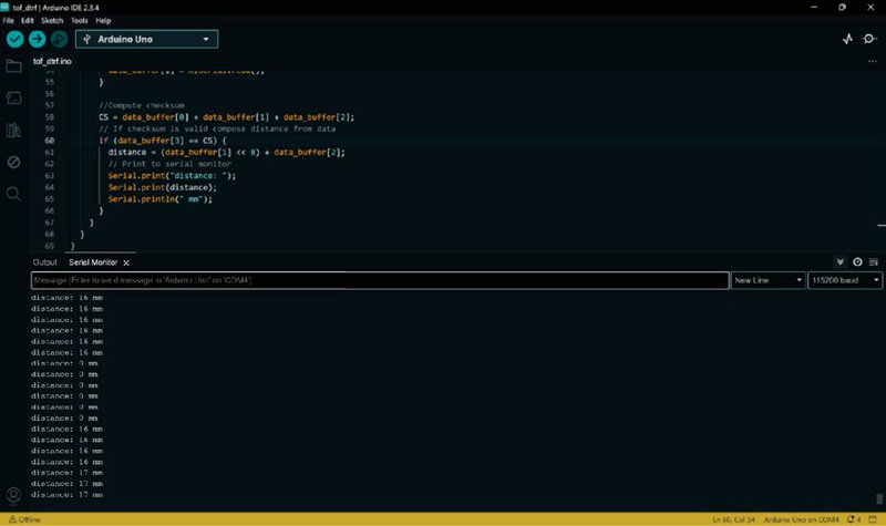
Figure 14 Computational readings showing real-time distance variations of object from the sensor.
A prototypical setup was developed in real-time, using Arduino Uno synchronized with waterproof ultrasonic sensor, waterproof electromagnetic coil and a magnetometer to perceive the object. Figure 13 shows the zoomed in view of the placed sensor along with the object and the connections. Figure 14 shows the real-time distance variations of object from the sensor. From the computations obtained in real-time, it is inferred that the continuous beeping in the magnetometer reveals continuous motion of a ferromagnetic material towards the sensor.
6 Conclusion
Underwater exploration is a field that requires continuous research and the development of new techniques. Traditional methods, such as imaging or videography, often fail in low-visibility underwater regions and do not account for seafloor topography or acoustic propagation. These limitations make them less effective in deep-sea environments, where conditions are harsh and visibility decreases with depth. To address these challenges, we adopt a different approach that relies on acoustic sensing rather than cameras. Sensors are strategically distributed in a grid pattern, enabling efficient detection through sound waves. The system leverages geometric mapping techniques, such as Delaunay’s Convex Hull, to reconstruct object shapes; fundamental principles of magnetic field balancing, such as the law of magnetic equilibrium; and motion tracking via the Doppler effect. By integrating these techniques, the system can accurately perceive objects even in deeper regions where cameras and AUVs are ineffective.
For future work, we aim to expand the sensor network, enhance real-time data transmission, and integrate advanced technologies to achieve smarter and more robust underwater object detection.
Acknowledgments
The authors would like to acknowledge the support provided by the Research Council of Norway through the INTPART DTRF project. They also sincerely thank the Ubiquitous Computing Laboratory (UbiComp) at the Indian Institute of Technology Indore for their invaluable assistance in providing computing facilities.
Disclosure/Conflict of Interest
The authors declare no conflicts of interest.
References
[1] D. Q. Huy, N. Sadjoli, A. B. Azam, B. Elhadidi, Y. Cai, and G. Seet, “Object perception in underwater environments: a survey on sensors and sensing methodologies,” Ocean Engineering, vol. 267, p. 113202, 2023.
[2] E. Felemban, F. K. Shaikh, U. M. Qureshi, A. A. Sheikh, and S. B. Qaisar, “Underwater sensor network applications: A comprehensive survey,” International Journal of Distributed Sensor Networks, vol. 11, no. 11, p. 896832, 2015.
[3] J. Aguzzi, L. Thomsen, S. Flögel, N. J. Robinson, G. Picardi, D. Chatzievangelou, N. Bahamon, S. Stefanni, J. Grinyó, E. Fanelli, et al., “New technologies for monitoring and upscaling marine ecosystem restoration in deep-sea environments,” Engineering, 2024.
[4] S. Tyagi, A. Shah, A. Srivastava, “Underwater object identification with edge computing paradigms,” in The 5th International Workshop on Big Data Driven Edge Cloud Services (BECS 2025) Co-located with the 25th International Conference on Web Engineering (ICWE 2025), June 30-July 3, 2025, Delft, Netherlands.
[5] J. Heidemann, M. Stojanovic, and M. Zorzi, “Underwater sensor networks: applications, advances and challenges,”Philosophical Transactions of the Royal Society A: Mathematical, Physical and Engineering Sciences, vol. 370, no. 1958, pp. 158–175, 2012.
[6] A. Pal, F. Campagnaro, K. Ashraf, M. R. Rahman, A. Ashok, and H. Guo, “Communication for underwater sensor networks: A comprehensive summary,” ACM Transactions on Sensor Networks, vol. 19, no. 1, pp. 1–44, 2022.
[7] Y. LeCun, L. Bottou, Y. Bengio, and P. Haffner, “Gradient-based learning applied to document recognition,” Proceedings of the IEEE, vol. 86, no. 11, pp. 2278–2324, 1998.
[8] J. Redmon, “You only look once: Unified, real-time object detection,” in Proceedings of the IEEE Conference on Computer Vision and Pattern Recognition, 2016.
[9] G. Bradski, “Learning OpenCV: Computer vision with the OpenCV library,” O’REILLY Google Scholar, vol. 2, pp. 334–352, 2008.
[10] T. O. Fossum, Ø. Sture, P. Norgren-Aamot, I. M. Hansen, B. C. Kvisvik, and A. C. Knag, “Underwater autonomous mapping and characterization of marine debris in urban water bodies,” arXiv preprint arXiv:2208.00802, 2022.
[11] S. Fayaz, S. A. Parah, and G. J. Qureshi, “Underwater object detection: architectures and algorithms–a comprehensive review,” Multimedia Tools and Applications, vol. 81, no. 15, pp. 20871–20916, 2022.
[12] M. A. Hayat, G. Yang, A. Iqbal, A. Saleem, and M. Mateen, “Comprehensive and comparative study of drowning person detection and rescue systems,” in 2019 8th International Conference on Information and Communication Technologies (ICICT), pp. 66–71, IEEE, 2019.
[13] L. Zhang, C. Li, and H. Sun, “Object detection/tracking toward underwater photographs by remotely operated vehicles (ROVs),” Future Generation Computer Systems, vol. 126, pp. 163–168, 2022.
[14] M.-J. Rakotosaona, P. Guerrero, N. Aigerman, N. J. Mitra, and M. Ovsjanikov, “Learning delaunay surface elements for mesh reconstruction,” in Proceedings of the IEEE/CVF Conference on Computer Vision and Pattern Recognition, pp. 22–31, 2021.
[15] C. M. Sorensen, “Magnetism,” Nanoscale Materials in Chemistry, pp. 169–221, Wiley Online Library, 2001.
[16] K. Toman, “Christian Doppler and the Doppler effect,” Eos, Transactions American Geophysical Union, vol. 65, no. 48, pp. 1193–1194, Wiley Online Library, 1984.
[17] Google, Google Earth, 2024. Available: https://earth.google.com/, Accessed: 2024-01-28.
[18] Advanced Converter, Find depth by coordinates, 2024. Webpage. Available: https://www.advancedconverter.com/map-tools/find-altitude-by-coordinates, Retrieved on January 28, 2025.
[19] J. Coulthard, QuikGrid (Version 5.4.4), 2007. Computer software. Last accessed on January 22, 2025.
[20] Tsuchiya, Acoustic Absorption Coefficient in Seawater, 2010. Webpage. Available: https://tsuchiya2.org/absorption/absorp_e.html, Retrieved on January 25, 2025.
[21] M. A. Ainslie and J. G. McColm, “A simplified formula for viscous and chemical absorption in sea water,”The Journal of the Acoustical Society of America, vol. 103, no. 3, pp. 1671–1672, Acoustical Society of America, 1998.
[22] Wikipedia Contributors, “Doppler Effect,” 2025. [Online]. Available: https://en.wikipedia.org/wiki/Doppler_effect. [Accessed: Feb. 5, 2025].
[23] J. Zhang, X. Xiang, and W. Li, “Advances in marine intelligent electromagnetic detection system, technology, and applications: A review,” IEEE Sensors Journal, vol. 23, no. 5, pp. 4312–4326, IEEE, 2021.
[24] Wikipedia Contributors, “Diamagnetism, Paramagnetism, and Ferromagnetism,” 2025. [Online]. Available: https://en.wikipedia.org/wiki/Diamagnetism, https://en.wikipedia.org/wiki/Paramagnetism, https://en.wikipedia.org/wiki/Ferromagnetism. [Accessed: Feb. 5, 2025].
Biographies

Shekhar Tyagi holds bachelor’s and master’s degrees in computer science and engineering. He is currently pursuing his doctoral degree in computer science and engineering at the Indian Institute of Technology Indore. His research interests include edge computing, IoT security in resource-constrained environments, and machine learning.

Akshat Shah holds a bachelor’s degree in computer science and engineering. He is currently working as a data engineer in the Data and AI Division at Infocepts, India. Previously, he interned at the Ubiquitous Computing Laboratory in the Department of Computer Science and Engineering at the Indian Institute of Technology Indore. His research interests include edge computing and machine learning.

Abhishek Srivastava is a professor in the discipline of computer science and engineering at the Indian Institute of Technology Indore. He completed his Ph.D. in 2011 from the University of Alberta, Canada. Abhishek’s group at IIT Indore has been involved in research on service-oriented systems most commonly realized through web-services. More recently, the group has been interested in applying these ideas in the realm of Internet of Things. The ideas explored include coming up with technology agnostic solutions for seamlessly linking heterogeneous IoT deployments across domains. Further, the group is also delving into utilizing machine learning adapted for constrained environments to effectively make sense of the huge amounts of data that emanate from the vast network of IoT deployments.
Journal of Web Engineering, Vol. 25_3, 325–350
doi: 10.13052/jwe1540-9589.2532
© 2026 River Publishers