Spatio-temporal Mamba for User Mobility Prediction in Mobile Edge Computing
Jeonghwa Lee1, Eunjeong Ju1, Duksan Ryu1,*, Suntae Kim1 and Jongmoon Baik2
1Department of Software Engineering, Jeonbuk National University, Jeonju, South Korea
2School of Computing, Korea Advanced Institute of Science and Technology (KAIST), Daejeon, South Korea
dlwjdghk133@jbnu.ac.kr; jeju3146@jbnu.ac.kr; duksan.ryu@jbnu.ac.kr; stkim@jbnu.ac.kr; jbaik@kaist.ac.kr
*Corresponding Author
Received 30 October 2025; Accepted 15 December 2025
Abstract
In mobile edge computing (MEC), frequent server handovers due to user mobility increase latency and degrade quality of service (QoS). This study enhances MEC service stability by predicting user mobility for efficient server transitions. The proposed spacio-temporal (ST)-Mamba model combines Mamba (state-space encoder) and a gated recurrent unit (GRU) in parallel to capture both long-term and short-term dependencies, while Fourier feature embedding enriches spatial-temporal representation. Experiments show that ST-Mamba achieves about 9–10% lower root mean square error (RMSE) and mean absolute error (MAE) than long short-term memory (LSTM), GRU, and Transformer baselines, with statistically significant improvements confirmed by Welch’s t-test. These results demonstrate that hybrid state space model (SSM)–RNN architectures are promising for mobility-aware QoS optimization in MEC, with future work extending to real-world and multi-user settings.
Keywords: Mobile edge computing (MEC), mobility prediction, Mamba, GRU, quality of service (QoS), sequence modeling.
1 Introduction
Mobile edge computing (MEC) is a paradigm that deploys computing resources closer to end users, significantly reducing latency compared to traditional cloud systems. This enables latency-critical applications such as AR/VR, autonomous driving, and smart cities, where millisecond-level responsiveness and stable quality of service (QoS) are essential [1, 2, 3, 4, 5].
However, user mobility frequently causes server handovers, which increase network load and lead to QoS degradation [6, 7, 8, 9, 10, 11]. In highly dynamic environments, such as vehicle or VR-based scenarios, unpredictable user movement leads to latency and unstable connections. Hence, accurate mobility prediction is crucial for proactive server management and consistent QoS in MEC environments [4, 5, 9, 12, 13, 14]. Early approaches, including Markov and probabilistic models, were limited in capturing long-term dependencies [15, 16, 17]. Later, RNN-based models such as LSTM and GRU improved temporal modeling but still suffered from vanishing gradients and high computational costs for long sequences [18, 19, 20]. Transformer-based architectures achieved superior spatiotemporal modeling through self-attention, yet their quadratic complexity () limits scalability in real-time MEC applications [10, 21, 22]. A representative example of Transformer-based work is the BERT-M model, which predicts the next connected server from past edge-connection sequences [23]. Although BERT-M efficiently captures contextual dependencies, it relies on discrete server identifiers instead of continuous trajectories, limiting spatial continuity and fine-grained QoS analysis. Moreover, the high computational complexity of the Transformer restricts real-time applicability. To address these limitations, recent studies have explored state space model (SSM)-based architectures such as Mamba, which achieve Transformer-level sequence modeling with linear complexity () [10, 22, 24]. These models can efficiently process large-scale mobility logs, but most existing works still focus solely on coordinate accuracy without linking prediction to MEC-level performance.
This paper proposes a ST-Mamba model that integrates Mamba with GRU to jointly capture long- and short-term mobility dependencies. In addition, last-step local features and temporal embeddings are incorporated to better represent spatial-temporal dynamics. The main contributions are as follows:
• This work is the first to apply the Mamba architecture to mobility prediction in MEC environments. The proposed model combines Mamba’s long-range dependency learning capability with GRU’s short-term sequential modeling, achieving efficient and accurate trajectory prediction.
• A large-scale dataset derived from Shanghai Telecom logs is built to reflect realistic MEC mobility patterns.
• The predicted coordinates are used to identify the nearest MEC server, validating the spatial reliability and potential QoS benefits of accurate mobility prediction.
The remainder of this paper is organized as follows. Section 2 reviews related work, Section 3 describes the proposed model, Section 4 explains the experimental setup, and Section 5 presents the results. Section 6 discusses threats to validity, and Section 7 concludes the paper.
2 Related Work
This section presents an overview of mobile edge computing (MEC) and mobility prediction, highlighting recent deep learning-based approaches and their limitations in dynamic MEC environments.
2.1 Overview of MEC and Mobility Prediction
Mobile edge computing (MEC) deploys computing resources closer to end users, significantly reducing latency and enabling real-time services in applications such as autonomous driving and AR/VR [7]. However, continuous user mobility in MEC environments causes frequent server handovers, which increase network load and degrade quality of service (QoS) [8, 9].
To mitigate this, several studies have proposed mobility prediction-based approaches for proactive server selection and handover management [25]. Deep learning models such as LSTM and GRU have outperformed traditional Markov chain-based methods, enhancing trajectory prediction and QoS in real-world environments [7, 26]. ConvLSTM and deep reinforcement learning (DRL) have also been applied to jointly optimize offloading and handover decisions [9, 11]. Despite these advances, large-scale mobility data still poses challenges due to high computational complexity and strict latency requirements [10, 27]. Recent research emphasizes integrating mobility prediction with server selection and offloading into unified frameworks to ensure consistent QoS in dynamic MEC scenarios [28].
2.2 Evolution of Time-series Models for Mobility Prediction
Early mobility prediction methods, including Markov chains and ARIMA, effectively modeled short-term mobility but failed to capture complex long-term dependencies [15, 18]. RNN-based architectures, particularly LSTM and GRU, improved temporal dependency modeling through gating mechanisms, yet their performance degraded for long sequences and incurred high computational costs [18, 29]. Transformer architectures later gained attention for their ability to model long-range dependencies via self-attention [30, 31].
However, their quadratic computational complexity limits their scalability for real-time MEC applications. Our previous study, BERT-M, applied a Transformer-based architecture for MEC server prediction using edge connection logs. Although BERT-M captured contextual dependencies effectively, it struggled to handle coordinate-based mobility trajectories and real-time processing due to the high computational cost of the Transformer. Recently, state space model (SSM)-based architectures such as Mamba have emerged as efficient alternatives to Transformers, maintaining similar modeling capacity with linear computational complexity [32, 33]. Mamba achieves hardware-efficient linear-time computation, providing up to 5× faster inference and lower memory usage than Transformers. These advantages make SSM-based models highly suitable for low-latency MEC environments. Table 1 gives a comparison of mobility prediction models.
Table 1 Comparison of mobility prediction models
| Model | Key characteristics | Strengths/limitations |
| LSTM | Gated recurrent design; sequence learning. () | + Learns long-term dependencies; strong temporal modeling. – Slow training; high computation cost. |
| GRU | Simplified gating; fewer parameters. () | + Fast convergence; efficient computation. – Weak for very long-range dependencies. |
| Transformer | Self-attention; global context learning. () | + Excellent spatial-temporal representation; parallel training. – High computational cost; low real-time suitability. |
| SSM (Mamba) | State-space linear recurrent update. () | + High throughput; low latency; memory-efficient. – Early-stage research; limited mobility applications. |
Building upon this evolution, the present study extends the BERT-M model by evolving the Transformer-based architecture into an SSM (Mamba)-based framework. The proposed ST-Mamba integrates Mamba’s efficient long-range dependency modeling with GRU’s short-term sequence learning, improving both accuracy and real-time prediction capability in MEC environments.
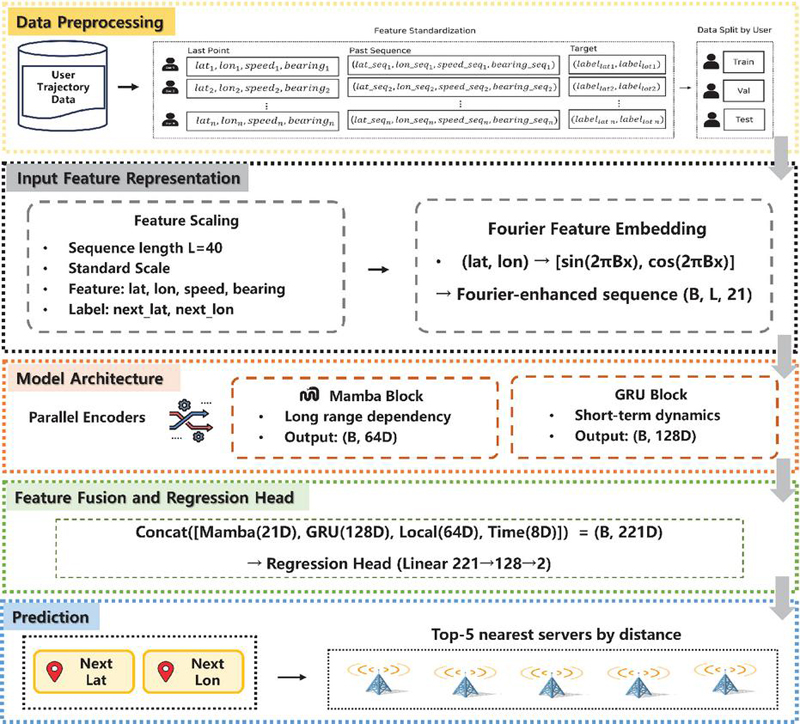
Figure 1 Overall architecture.
3 Methodology
We propose the spatio-temporal Mamba (ST-Mamba) model for efficient spatio-temporal mobility prediction. Figure 1 illustrates its overall architecture. From a system perspective, the proposed ST-Mamba is designed for deployment in mobile edge computing (MEC) environments. We conceptually assume a separated training and inference paradigm, in which model training is performed offline using historical user mobility logs, while the trained model can be deployed at MEC edge servers or regional edge controllers to perform online mobility inference. This deployment assumption reflects a common practice in MEC systems, enabling proactive server handover and service migration while satisfying low-latency requirements.
3.1 Data Preprocessing
Data preprocessing includes sequence generation, feature normalization, and user-level data splitting to ensure consistent scaling and prevent data leakage across users (Algorithm 1).
Algorithm 1 Data preprocessing pipeline.
Require: Raw mobility dataset with user trajectories
Ensure: Processed dataset for model training
1: Input: Raw dataset containing columns [latitude_seq, longitude_seq, speed_seq, bearing_seq, hour_seq].
2: Output: Processed DataFrame with structured input–target pairs.
3: Step 1: Sequence truncation
4: for each feature column in do
5: Keep only the last elements of each sequence using fast_tail_eval().
6: end for
7: Step 2: Sample construction
8: for each user in do
9:Split each trajectory into input and label pairs.
10:Extract last-step features: latitude, longitude, speed, bearing, and hour.
11: end for
12: Step 3: Normalization
13: Fit a StandardScaler on training users for [lat, lon, speed, bearing, label_lat, label_lon].
14: Apply the same scaling parameters to all sequence features.
15: Step 4: User-level split
16: Split unique users into 64% train, 16% validation, and 20% test (no overlap).
17: Construct datasets accordingly.
18: return
3.1.1 Sequence generation
For each user, consecutive connection records were converted into a sequence form (lines 3–11). The sequence length was set to 40 in the main experiment. The last position in each sequence was designated as the prediction target, while the previous time steps were used as the input. In other words, the sequence was structured as an input–target pair of the form:
This formulation enables the model to learn temporal dependencies and spatial transitions in user trajectories.
3.1.2 Normalization
Continuous variables such as latitude, longitude, speed, and bearing were normalized using the StandardScaler method to have zero mean and unit variance (lines 12–14). To prevent data leakage, the normalization parameters (mean and standard deviation) were computed exclusively from the training set and then applied to the validation and test sets.
3.1.3 User-level data splitting
The dataset was divided by users (lines 15–18), assigning 80% for training, 10% for validation, and 10% for testing. This split prevents data overlap among users and improves model generalization.
3.2 Input Feature Representation
3.2.1 Sequential input
The model input is composed of a five-dimensional feature vector that represents each time step in chronological order (Algorithm 2, lines 2a–2b):
| (1) |
Among these features, the spatial coordinates (latitude and longitude) are transformed usingFourier feature embedding to incorporate spatial periodicity. The Fourier transformation projects the spatial information into multiple frequency domains, allowing the model to represent fine-grained positional variations:
| (2) |
where is a learnable projection matrix and . After applying the Fourier embedding (16 dimensions), the final input sequence is composed of features in total, combining spatial, temporal, and motion attributes.
3.2.2 Last-step spatial and temporal features
At the final time step , the model additionally incorporates the most recent movement state as auxiliary inputs. The last-step spatial and motion features,including latitude, longitude, speed, and bearing form a four-dimensionallocal feature vector, which is transformed into a 64-dimensional representation through a multi-layer perceptron (MLP)(lines 2d–2e). In addition, the temporal feature (hour) is embedded via a learnable embedding layer into an eight-dimensional vector, capturing the periodic characteristics of daily mobility patterns.
3.3 Model Architecture
The proposed ST-Mamba architecture consists of a Mamba encoder, a GRU encoder, and a feature fusion module with an MLP regression head (lines 2c, 2f–2g).
Algorithm 2 ST-Mamba training and evaluation pipeline.
Require: Processed datasets
Ensure: Trained model and evaluation metrics (RMSE, MAE, )
1: Step 1. Dataset preparation Load into DataLoaders (batch size = 512).
2: Step 2. Model architecture
1. Input construction: For each sequence, form .
2. Fourier embedding: Apply sinusoidal projection to → .
3. Sequence encoding:
• Mamba encoder: Input → Output .
• GRU encoder: Input → Output .
4. Local features: Concatenate , pass through local MLP → .
5. Temporal embedding: Encode → .
6. Feature fusion: Concatenate all representations
7. Regression head: Pass through MLP → predict .
3: Step 3. Training configuration Optimizer: AdamW (), Loss: MSE, Epochs: 30, Patience: 5, AMP enabled.
4: Step 4. Multi-seed evaluation For each seed , fix seed, train on , evaluate on , and record (RMSE, MAE, ).
5: Step 5. Result aggregation Compute mean std of metrics across 10 runs and sequence length .
3.3.1 Mamba encoder
The Mamba encoder is based on a state space model (SSM) formulation, which efficiently captures long-range sequence dependencies through linear recurrent state updates. For an input sequence , Mamba performs the following state transitions:
| (3) | ||
where denotes the hidden state at time step , and , , , and are learnable transition matrices.
Through this linear sequence modeling process, the encoder maintains Transformer-level sequence representation capability while reducing computational complexity to . Intuitively, this formulation allows the model to propagate and aggregate spatial-temporal signals efficiently across long sequences without explicit attention mechanisms. The final hidden state captures the global mobility context over the entire trajectory.
3.3.2 GRU encoder
The GRU encoder is designed to model short-term dependencies within the mobility sequence. By applying a gating mechanism, it effectively summarizes recent movement patterns and local transitions in user behavior. The final hidden state represents the local mobility trend for each user. The hidden size of the GRU was set to 128 in all experiments.
Unlike single-model architectures, the proposed ST-Mamba design combines the complementary strengths of both components. While the Mamba encoder efficiently captures long-range mobility dependencies through linear state updates, it may underrepresent short-term local transitions that occur frequently in real-world user movements. Conversely, the GRU encoder excels at modeling recent, fine-grained variations in mobility but has limited capacity to retain information over long sequences. By integrating both encoders in parallel and fusing their latent representations, the proposed architecture achieves a balance between global contextual awareness and local adaptability, which is crucial for accurate and stable mobility prediction in MEC environments.
3.3.3 Feature fusion and regression head
The outputs from both encoders are integrated to combine global and local representations using a simple concatenation approach. This process can be expressed as follows:
| (4) |
Here, denotes a 64-dimensional feature vector extracted from the spatial MLP at the last time step, and represents an 8-dimensional temporal embedding.
In the proposed ST-Mamba model, the output dimensions of each component are as follows: Mamba encoder (21D), GRU encoder (128D), local MLP (64D), and time embedding (8D). These four feature vectors are concatenated to form a unified 221-dimensional representation vector.
The fused vector is then passed to a multi-layer perceptron (MLP) regression head with ReLU activation. The regression head follows a linear (2211282) structure, where the first hidden layer (128D) applies non-linear activation, and the final two-dimensional output layer predicts the next latitude and longitude coordinates. The model is trained using the mean squared error (MSE) loss function:
| (5) |
where and denote the predicted and ground-truth coordinates, respectively.
4 Experimental Setup
All experiments in this study were conducted in a unified offline Python-based environment, where the proposed model and all baseline models were trained and evaluated under identical hardware and software settings to ensure fair comparison and reproducibility.
4.1 Research Questions
To evaluate the effectiveness of the proposed ST-Mamba, we define the following four research questions:
• RQ1. Effectiveness of the ST-Mamba: Does the proposed ST-Mamba outperform single-component models in terms of coordinate prediction accuracy?
• RQ2. Contribution of feature groups: Among latitude/longitude, speed, bearing, local features, and time embeddings, which component contributes most to performance improvement?
• RQ3. Sensitivity to sequence length and scaling: How do different sequence lengths () and normalization methods affect prediction accuracy and training stability?
• RQ4. Distance-based evaluation for predicted user–server proximity: How effective is the nearest-server selection based on the predicted user coordinates in replicating the ground-truth server assignments?
4.2 Dataset
The Shanghai Telecom server location data used in this study are publicly available from external sources, while the user mobility location data were synthetically generated based on the server coverage area and mobility constraints. To simulate a realistic MEC (mobile edge computing) environment, we constructed a user mobility trajectory dataset based on the server location data (Shanghai Telecom). The ST-Mamba model utilizes the full user mobility dataset during the training phase, while during inference it takes as input only the most recent L-step mobility history of each individual user. In other words, the next location can be predicted using only partial and recent trajectory information, without requiring access to the entire historical dataset.
1. User data generation based on server range. We first extracted the maximum and minimum values of latitude and longitude from the MEC server dataset to define the spatial boundary for generating user coordinates. This ensures that all user locations are created within the actual geographical region covered by existing servers. The generated user coordinates serve as the base data for the subsequent filtering and sequence construction steps.
2. User filtering within the server coverage radius. To select only users located within the 50 km radius of a server, we employed the BallTree structure using the Haversine distance metric. For each user coordinate, the distance to all server locations was computed, and only those within 50 km were retained.
3. Trajectory sequence construction. For each user, we constructed a trajectory sequence consisting of the 60 nearest spatially adjacent coordinates. The BallTree was again used to identify the 60 closest points, which were then ordered chronologically to form a continuous movement sequence. Each trajectory sequence includes five attributes: latitude, longitude, speed, bearing, and hour. To simulate temporal diversity, each user sequence was randomly assigned a time-of-day type (morning, day, or night), and corresponding hour values were generated according to the assigned period.
4. Outlier removal and final filtering. Some sequences exhibited unrealistic jumps (e.g., movements over 50 km between consecutive points). To address this, we applied Haversine distance-based outlier detection and removed all users containing such anomalies. If the distance between two consecutive coordinates exceeded 50 km, the corresponding trajectory was discarded. This cleaned dataset served as the final input for all experiments (RQ1–RQ4). In particular, RQ4 utilized the predicted mobility trajectories to perform nearest server extraction (server association) using the Shanghai Telecom server location dataset.
4.3 Baselines
To quantitatively evaluate the effectiveness of the proposed hybrid model, we compare it against four representative baseline models that are widely used in sequence modeling tasks. All models are trained on the same user trajectory dataset but differ in how they capture temporal dependencies within the input sequences.
1. Mamba (state-space model-based). Mamba is a recent state-space model (SSM) architecture that maintains Transformer-level capability for learning long-range dependencies while significantly reducing computational complexity. In this study, Mamba processes the entire input sequence, and the final state representation is used to predict the next coordinates (latitude and longitude). This model serves as a benchmark for evaluating the balance between efficiency and long-sequence modeling capability.
2. GRU (gated recurrent unit). The GRU is a lightweight variant of the recurrent neural network (RNN) that effectively models short-term temporal dependencies with fewer parameters. The model encodes the input trajectory sequence and predicts the next coordinates based on the final hidden representation. It is used as a baseline to verify the stability and efficiency of short-sequence learning.
3. LSTM (long short-term memory). LSTM features a more complex gating mechanism than the GRU, enabling it to better preserve long-term temporal information. The model encodes temporal transitions within the input sequence and predicts the subsequent coordinates (latitude and longitude) based on the learned representation. This baseline is included to compare the representational capability of LSTM against the GRU.
4. Transformer encoder. The Transformer encoder leverages self-attention mechanisms to capture global dependencies across all time steps in the sequence. In this study, positional encoding is applied to incorporate sequential order information, and the encoded representation is used to predict the next coordinates. This model serves as a strong baseline for evaluating the performance of long-range dependency modeling.
4.4 Evaluation Metrics
4.4.1 Regression metrics
To quantitatively assess coordinate prediction accuracy, we adopt three standard measures: RMSE, MAE, and .
• Root mean squared error (RMSE)
| (4) |
where denotes the predicted coordinates and denotes the ground-truth coordinates. RMSE emphasizes larger errors by squaring deviations, providing a measure of overall predictive accuracy.
• Mean absolute error (MAE)
| (5) |
MAE measures the average magnitude of prediction errors regardless of direction and provides an intuitive interpretation of the model’s typical deviation from actual coordinates.
• Coefficient of determination ()
| (6) |
where represents the mean of all ground-truth coordinates. A higher indicates that the model explains a larger portion of the data variance.
4.4.2 Evaluation of predicted user–server proximity
To assess how accurately the predicted user locations align spatially with nearby MEC servers, we evaluate three complementary metrics: location error (LocErr),mean server distance (SrvDist_Mean), and server matching accuracy (Match@1).
• Location error (LocErr)
| (7) |
where denotes the Haversine distance between the predicted coordinate and the ground-truth coordinate . A smaller LocErr indicates higher spatial accuracy in predicting the user’s actual position.
• Mean server distance (SrvDist_Mean)
| (8) |
where denotes the nearest MEC server to the predicted coordinate. This metric measures the average proximity between predicted user positions and their nearest servers, with smaller values indicating more geographically efficient predictions.
• Server matching accuracy (Match@1)
| (9) |
where represents the nearest MEC server to a given coordinate. Match@1 quantifies the percentage of cases where the predicted and true user positions are assigned to the same nearest server, reflecting the model’s alignment consistency.
5 Experimental Results
5.1 RQ1. Performance of the Mamba-based Framework
Table 2 Performance comparison of ST-Mamba and baseline models (10 seeds). Values represent mean std. Bold indicates the best results
| Model | RMSE (↓) | MAE (↓) | (↑) |
| Mamba | 0.03375 0.0303 | 0.02022 0.0232 | 0.9171 0.1753 |
| GRU | 0.02238 0.0011 | 0.01239 0.00036 | 0.9798 0.0018 |
| LSTM | 0.02195 0.0008 | 0.01208 0.00035 | 0.9806 0.0011 |
| Transformer | 0.02775 0.0015 | 0.01561 0.00054 | 0.9688 0.0029 |
| ST-Mamba (ours) | 0.02015 0.00068 | 0.01134 0.00017 | 0.9835 0.00083 |
Table 3 Welch’s t-test results for statistical significance between ST-Mamba and baseline models (10 seeds). Bold indicates statistically significant results ()
| Model | |||
| Mamba | 0.1895 | 0.2579 | 0.2615 |
| GRU | 0.00007 | 0.00000 | 0.00004 |
| LSTM | 0.00005 | 0.00000 | 0.00000 |
| Transformer | 0.00000 | 0.00000 | 0.00000 |
Table 2 presents the performance comparison among all baseline models and the proposed ST-Mamba model under the condition of sequence length and the StandardScaler normalization. As shown in both the table and the bar chart, the ST-Mamba model consistently achieves the lowest RMSE and MAE values and the highest , indicating superior coordinate prediction accuracy.
Specifically, the ST-Mamba model yields an RMSE of 0.02015 and an MAE of 0.01134, outperforming GRU and LSTM by approximately 9–10% on average. This improvement demonstrates that combining Mamba’s state-space representation with GRU’s recurrent dynamics and a lightweight MLP effectively enhances both short-term and long-term dependency modeling.
In contrast, the standalone Mamba and Transformer baselines show relatively higher error values, confirming their limited ability to capture localized temporal variations when used independently. Additionally, to verify the reliability of the observed improvements, a Welch’s t-test was performed on the results from 10 different random seeds (Table 3). The ST-Mamba model showed statistically significant improvements over GRU, LSTM, and Transformer baselines with , demonstrating that the performance gains are statistically reliable rather than resulting from random variation.
5.2 RQ2. Contribution of Feature Groups
To examine how different input features influence prediction performance, we conducted a feature contribution analysis by incrementally adding feature groups. The experimental conditions are defined as follows:
• a_latlon: Uses only latitude and longitude as input.
• b_latlon+speed: Adds speed information to the latitude and longitude inputs.
• c_speed+bearing: Adds both speed and bearing (direction) features.
• d_local_on: Incorporates local contextual features in addition to the above inputs.
• f_timeemb_on: Adds temporal embedding (time-of-day) information.
• g_laststep_only: Uses only the last-step features (non-sequential input) for comparison.
Table 4 Ablation study results for feature group contribution
| Condition | RMSE | MAE | |
| a_latlon | 0.020362 | 0.011221 | 0.983518 |
| b_latlon+speed | 0.020152 | 0.011099 | 0.983761 |
| c_speed+bearing | 0.020261 | 0.011106 | 0.983604 |
| d_local_on | 0.020205 | 0.011202 | 0.983676 |
| f_timeemb_on | 0.020738 | 0.011544 | 0.982810 |
| g_laststep_only | 0.026733 | 0.014091 | 0.971427 |
According to the results in Table 4, the configurationb (latlon+speed) achieved the lowest RMSE (0.02015), MAE (0.01110), and highest (0.98376), showing the best overall performance. This demonstrates that the inclusion of speed plays a crucial role in capturing short-term motion dynamics for more precise coordinate prediction.
In contrast, adding bearing or local context features resulted in negligible improvement, indicating that the combination of location and speed already contains most of the predictive information. Furthermore, the addition of time embedding slightly degraded performance, suggesting redundancy with existing motion-related features. Finally, the g (laststep only) model, which uses only the final step without sequential input, showed a significant performance drop, confirming the importance of temporal dependency.
5.3 RQ3. Sensitivity to Sequence Length and Scaling
Table 5 presents the performance comparison of the ST-Mamba (evaluated using the hybrid variant) across different sequence lengths () and normalization methods. As shown in the table, both sequence length and scaler choice have a clear impact on coordinate prediction performance. Among the three scalers, the Standard Scaler achieved the best overall results, particularly when , showing the lowest RMSE (0.02021) and the highest (0.9835). This indicates that using a moderate sequence length allows the model to effectively capture temporal dependencies while preventing overfitting to short-term fluctuations. In contrast, the MinMax Scaler produced relatively lower performance, likely due to its sensitivity to outliers, whereas the Robust Scaler showed consistent results across all sequence lengths, demonstrating its robustness to input variations. Overall, the combination of the Standard Scaler and a sequence length of approximately provides the most balanced configuration between prediction accuracy and model stability.
Table 5 Performance comparison across different scalers and sequence lengths ()
| Scaler | RMSE | MAE | ||
| MinMax | 10 | 0.02749 | 0.01471 | 0.9701 |
| 20 | 0.02854 | 0.01473 | 0.9682 | |
| 30 | 0.02829 | 0.01502 | 0.9684 | |
| 40 | 0.02833 | 0.01469 | 0.9684 | |
| 50 | 0.02930 | 0.01606 | 0.9664 | |
| 60 | 0.02807 | 0.01450 | 0.9688 | |
| Robust | 10 | 0.02127 | 0.01166 | 0.9820 |
| 20 | 0.02071 | 0.01154 | 0.9829 | |
| 30 | 0.02065 | 0.01143 | 0.9830 | |
| 40 | 0.02108 | 0.01169 | 0.9824 | |
| 50 | 0.02076 | 0.01170 | 0.9828 | |
| 60 | 0.02085 | 0.01148 | 0.9827 | |
| Standard | 10 | 0.02123 | 0.01161 | 0.9820 |
| 20 | 0.02062 | 0.01142 | 0.9829 | |
| 30 | 0.02067 | 0.01139 | 0.9828 | |
| 40 | 0.02021 | 0.01134 | 0.9835 | |
| 50 | 0.02042 | 0.01125 | 0.9833 | |
| 60 | 0.02056 | 0.01152 | 0.9830 |
5.4 RQ4. Distance-based Evaluation for Predicted User–Server Proximity
Table 6 Comparison of spatial accuracy and server proximity metrics across models
| LocErr_MAE | LocErr_Median | SrvDist_Mean | SrvDist_Median | ||
| Model | (km) | (km) | (km) | (km) | Match@1 |
| ST-Mamba | 1.7644 | 1.2735 | 1.0059 | 0.5703 | 0.1557 |
| Mamba | 10.7440 | 8.2308 | 0.6776 | 0.3942 | 0.0087 |
| GRU | 3.1025 | 1.6916 | 0.7247 | 0.5529 | 0.1198 |
| LSTM | 2.7007 | 1.6682 | 0.7083 | 0.5364 | 0.1157 |
| Transformer. | 3.1500 | 1.7488 | 0.6905 | 0.5321 | 0.1067 |
Table 6 presents the results of the distance-based evaluation between the predicted user coordinates and the nearest MEC server locations. Among all models, the ST-Mamba achieves the best overall balance: it records the lowest location error (1.76 km MAE, 1.27 km median) and the highest server-level consistency (Match@1 = 0.1557), indicating reliable spatial alignment between user prediction and server distribution. Although the standalone Mamba model yields the smallest server proximity distances, its high location error and very low Match@1 suggest that its predicted coordinates are not spatially consistent with actual mobility patterns. Thus, the proposed ST-Mamba provides a more robust and spatially meaningful representation for mobility-aware MEC applications.
6 Threats to Validity
Although the proposed ST-Mamba model was empirically validated through extensive experiments, several potential threats to validity remain.
Internal validity. The model’s performance may be affected by hyperparameter configurations such as learning rate, sequence length, and embedding dimensions, which were explored within a limited range. While random seed variation cannot be completely eliminated, this study mitigated such variability by averaging the results over ten repeated experiments.In addition, the proposed ST-Mamba adopts a hybrid architecture that combines a Mamba-based state-space model and a GRU, which may increase the number of parameters and structural complexity compared to single-encoder models.
External validity. The experiments were conducted using a synthetically generated mobility dataset designed to emulate an MEC environment. Although this dataset is suitable for controlled evaluation, it may not fully capture real-world mobility behaviors or network dynamics. Additionally, the assumption of fixed MEC server locations and a constant 50 km coverage radius oversimplifies the complexity of real deployments with dynamic server placement and variable network conditions.
7 Conclusion
This study proposed the ST-Mamba model for user mobility prediction in MEC. The model integrates the Mamba (state-space encoder) and GRU (recurrent encoder) in parallel to jointly capture long-term dependencies and short-term mobility patterns, while Fourier feature embedding and temporal-spatial modules enhance representation capability.
Experimental results showed that ST-Mamba consistently outperforms baseline models in prediction accuracy and stability. The findings highlight the importance of sequence length and normalization in maintaining balanced temporal context and feature scaling.
Overall, this work suggests that hybrid architectures combining state space models (SSM) and recurrent neural networks (RNNs) can form the basis of future mobility-aware QoS optimization frameworks. Future work will focus on applying the model to real-world mobility data, integrating it with QoS-driven MEC policies, and exploring multi-user interference scenarios.
Acknowledgements
This work was supported by the MSIT (Ministry of Science and ICT), Korea, under the ITRC (Information Technology Research Center) support program (IITP-2026-RS-2020-II201795, 25%) supervised by the IITP (Institute for Information & Communications Technology Planning & Evaluation) and the High-Performance Computing Support Project, funded by the Government of the Republic of Korea (Ministry of Science and ICT)(RQT-25-070067, 25%) and the Regional Innovation System & Education (RISE) program through the Jeonbuk RISE Center, funded by the Ministry of Education (MOE) and the Jeonbuk State, Republic of Korea (2025-RISE-13-JBU, 25%) and the Institute of Information & Communications Technology Planning & Evaluation (IITP)-Innovative Human Resource Development for Local Intellectualization program grant funded by the Korea government (MSIT) (IITP-2026-RS-2024-00439292, 25%).
References
[1] Elbamby, M. S., C. Perfecto, M. Bennis, and K. Doppler. 2018. Toward low-latency and ultra-reliable virtual reality. IEEE Network. 32(2): 78–84.
[2] Zhou, P. Y., Y. Zhang, X. Wang, et al. 2024. 5G MEC computation handoff for mobile augmented reality. In Proceedings of the IEEE International Conference on Metaverse Computing, Networking, and Applications (MetaCom). IEEE. pp. 1–6.
[3] Ranaweera, P., A. Jurcut, and M. Liyanage. 2021. MEC-enabled 5G use cases: A survey on security vulnerabilities and countermeasures. ACM Computing Surveys (CSUR). 54(9): 1–37.
[4] Bozkaya, E. 2023. Digital twin-assisted and mobility-aware service migration in mobile edge computing. Computer Networks. 231: 109798.
[5] Alsahfi, T., et al. 2025. Optimizing healthcare big data performance through regional computing. Scientific Reports. 15(1): 3129.
[6] Tran, T. P., and M. Yoo. 2024. Mobility-aware Service Migration in MEC System. In Proceedings of the 2024 International Conference on Information Networking (ICOIN). IEEE. pp. 653–656.
[7] Yang, R., H. He, and W. Zhang. 2021. Multitier service migration framework based on mobility prediction in mobile edge computing. Wireless Communications and Mobile Computing. 2021(1): 6638730.
[8] Jahandar, S., et al. 2025. Handover decision with multi-access edge computing in 6G networks: A survey. Results in Engineering. 103934.
[9] Mehrabi, M., H. Salah, and F. H. P. Fitzek. 2019. A survey on mobility management for MEC-enabled systems. In Proceedings of the IEEE 2nd 5G World Forum (5GWF). IEEE. pp. 259–263.
[10] Singha, N. R., N. Sarma, and D. K. Saikia. 2025. TMLpSA-MEC: Transformer-based Mobility Aware Periodic Service Assignment in Mobile edge computing. Computer Networks. 111329.
[11] Loutfi, S. I., et al. 2024. An overview of mobility awareness with mobile edge computing over 6G network: Challenges and future research directions. Results in Engineering. 23: 102601.
[12] Xu, G., et al. 2016. A survey for mobility big data analytics for geolocation prediction. IEEE Wireless Communications. 24(1): 111–119.
[13] Bhadani, A. K., and D. Jothimani. 2016. Big data: challenges, opportunities, and realities. In Effective Big Data Management and Opportunities for Implementation. pp. 1–24.
[14] Fattore, U., et al. 2020. AutoMEC: LSTM-based user mobility prediction for service management in distributed MEC resources. In Proceedings of the 23rd International ACM Conference on Modeling, Analysis and Simulation of Wireless and Mobile Systems. ACM.
[15] Kulkarni, V., et al. 2019. Examining the limits of predictability of human mobility. Entropy. 21(4): 432.
[16] Lu, X., et al. 2013. Approaching the limit of predictability in human mobility. Scientific Reports. 3(1): 2923.
[17] Qiao, Y., et al. 2018. A hybrid Markov-based model for human mobility prediction. Neurocomputing. 278: 99–109.
[18] Ma, Z., and P. Zhang. 2022. Individual mobility prediction review: Data, problem, method and application. Multimodal Transportation. 1(1): 100002.
[19] Brik, B., and A. Ksentini. 2021. Toward optimal MEC resource dimensioning for a vehicle collision avoidance system: A deep learning approach. IEEE Network. 35(3): 74–80.
[20] Zeng, Q., et al. 2025. Device-Driven Service Allocation in Mobile Edge Computing with Location Prediction. Sensors. 25(10): 3025.
[21] Marmat, A., and D. Thankachan. 2025. ML-driven latency optimization for mobile edge computing in fiber-wireless access networks. MethodsX. 103594.
[22] Zhang, X., et al. 2025. Pretraining-improved Spatiotemporal graph network for the generalization performance enhancement of traffic forecasting. Scientific Reports. 15(1): 27668.
[23] The 5th International Workshop on Big data driven Edge Cloud Services (BECS 2025) Co-located with the 25th International Conference on Web Engineering (ICWE 2025), June 30–July 3, 2025, Delft, Netherlands
[24] Liu, F., et al. 2025. Enhanced Mamba model with multi-head attention mechanism and learnable scaling parameters for remaining useful life prediction. Scientific Reports. 15(1): 7178.
[25] Singh, R., R. Sukapuram, and S. Chakraborty. 2023. A survey of mobility-aware multi-access edge computing: Challenges, use cases and future directions. Ad Hoc Networks. 140: 103044.
[26] Qin, Y., et al. 2025. Task offloading optimization in mobile edge computing based on a deep reinforcement learning algorithm using density clustering and ensemble learning. Scientific Reports. 15(1): 211.
[27] Bernad, C., et al. 2025. Towards Smart 6G: Mobility Prediction for Dynamic Edge Services Migration. Expert Systems with Applications. 129348.
[28] Tran, T. P., and M. Yoo. 2024. Mobility-aware Service Migration in MEC System. In Proceedings of the 2024 International Conference on Information Networking (ICOIN). IEEE. pp. 653–656.
[29] Xiao, Jue, Tingting Deng, and Shuochen Bi. 2024. “Comparative analysis of LSTM, GRU, and transformer models for stock price prediction.” proceedings of the international conference on digital economy, blockchain and artificial intelligence.
[30] Gunkel, Jonas, Andrea Tundis, and Max Mühlhäuser. 2024 “The Story of Mobility: Combining State Space Models and Transformers for Multi-Step Trajectory Prediction.” Proceedings of the 2nd ACM SIGSPATIAL International Workshop on Human Mobility Prediction Challenge.
[31] Qin, Zhenlin, et al. 2025 “TransGTE: a transformer-based model with geographical trajectory embedding for the individual trip destination prediction.” Expert Systems with Applications: 128159.
[32] Liu, Fugang, et al. 2025. “Enhanced Mamba model with multi-head attention mechanism and learnable scaling parameters for remaining useful life prediction.” Scientific Reports 15.1: 7178.
[33] Patro, Badri Narayana, and Vijay Srinivas Agneeswaran. 2025. “Mamba-360: Survey of state space models as transformer alternative for long sequence modelling: Methods, applications, and challenges.” Engineering Applications of Artificial Intelligence 159: 111279.
Biographies

Jeonghwa Lee received her B.Sc. degree in software engineering from Jeonbuk National University, Korea, in 2024. She is currently pursuing an M.Sc. degree in the Department of Software Engineering at Jeonbuk National University. Her research interests include software defect prediction, data analysis, and artificial intelligence.

Eunjeong Ju received her B.Sc. degree in software engineering from Jeonbuk National University, Korea, in 2024. She is currently pursuing an M.Sc. degree in the Department of Software Engineering at Jeonbuk National University. Her research interests include software engineering, data science, and artificial intelligence.

Duksan Ryu received his dual M.Sc. degrees in software engineering from KAIST, Korea, and Carnegie Mellon University, USA, in 2012, and his Ph.D. degree in computer science from KAIST in 2016. Since 2018, he has been an associate professor with the Department of Software Engineering at Jeonbuk National University. His research interests include AI/LLM-based software analysis, software defect prediction, software reliability, software metrics, and software quality assurance.

Suntae Kim received his M.Sc. and Ph.D. degrees in computer science and engineering from Sogang University, Korea, in 2007 and 2010, respectively. He is currently a professor in the Department of Software Engineering at Jeonbuk National University, Korea, and the head of the Visit Systems & Software Engineering Lab. His research interests include financial technology, blockchain and smart contracts, software engineering, and artificial intelligence.

Jongmoon Baik received his B.Sc. degree in computer science and statistics from Chosun University, Korea, in 1993, and his M.Sc. and Ph.D. degrees in Computer Science from the University of Southern California, USA, in 1996 and 2000, respectively. He worked as a Principal Research Scientist at Motorola Labs and is currently a professor in the School of Computing at KAIST. His research interests include software six sigma, software reliability, and software process improvement.
Journal of Web Engineering, Vol. 25_3, 417–440
doi: 10.13052/jwe1540-9589.2536
© 2026 River Publishers