Comparisons of Machine Learning Methods of Statistical Downscaling Method: Case Studies of Daily Climate Anomalies in Thailand
Kanawut Chattrairat1, Waranyu Wongseree2, and Adisorn Leelasantitham1,*
1Technology of Information System Management, Faculty of Engineering, Mahidol University, Thailand
2Department of Electrical and Computer Engineering, King Mongkut’s University of Technology North Bangkok, Thailand
E-mail: kanawut.cht@student.mahidol.ac.th; waranyu.wongseree@gmail.com; adisorn.lee@mahidol.ac.th
*Corresponding Author
Received 10 August 2020; Accepted 17 February 2021; Publication 12 July 2021
Abstract
The climate change which is essential for daily life and especially agriculture has been forecasted by global climate models (GCMs) in the past few years. Statistical downscaling method (SD) has been used to improve the GCMs and enables the projection of local climate. Many pieces of research have studied climate change in case of individually seasonal temperature and precipitation for simulation; however, regional difference has not been included in the calculation. In this research, four fundamental SDs, linear regression (LR), Gaussian process (GP), support vector machine (SVM) and deep learning (DL), are studied for daily maximum temperature (TMAX), daily minimum temperature (TMIN), and precipitation (PRCP) based on the statistical relationship between the larger-scale climate predictors and predictands in Thailand. Additionally, the data sets of climate variables from over 45 weather stations overall in Thailand are used to calculate in this calculation. The statistical analysis of two performance criteria (correlation and root mean square error (RMSE)) shows that the DL provides the best performance for simulation. The TMAX and TMIN were calculated and gave a similar trend for all models. PRCP results found that in the North and South are adequate and poor performance due to high and low precipitation, respectively. We illustrate that DL is one of the suitable models for the climate change problem.
Keywords: Global climate model (GCM), statistical downscaling (SD) method, linear regression (LR), Gaussian process (GP), support vector machine (SVM), deep learning (DL).
1 Introduction
Nowadays, global warming is widely gaining attention from many organizations because they are significantly affecting living lives. The climate change causes disaster such as flood, storm, and drought [1]. There are the collected temperature data in 20 years that has been continuously increased [2]. Moreover, the climate change impacts are not only sea-level increasing but also the greenhouse gas increase from the industrial revolution [3]. Thus, a climate model is essential for forecasting impact and discovering adaptation from climate change. There are many developments of climate models in previous researches such as large and small resolution climate model that has a resolution about over a hundred kilometers and less than ten kilometers, respectively [4]. Now, the development is not only about the area resolution but also necessary knowledge which improves the climate model and weather data measurement. Thus, reliable atmospheric sciences lead to the believed climate model.
The climate change directly affects not only disaster but also has an impact on agriculture [5–7], health [8, 9], and water source [10, 11]. As is well known, the climate forecast is extremely significant to agriculture. Thus, researchers have highly paid attention to precisely forecast climate for preparing solution, which can be determined by simulating the global climate model (GCM). It is the mathematic simulation that imitates circulation of mass and energy between climate global components under the global emission scenarios which are defined by Intergovernmental Panel on Climate Change (IPCC) for forecasting global climate [2]. However, the detail of GCM depends on technique and theory used to design and simulate which often cannot be fully represented due to lack of computing resources and input data. Thus, GCM should be speculated at global or continental scales for climatic conditions averaged at monthly, seasonal, annual, and longer time scales [12].
The first GCM was created in NOAA’s Geophysical Fluid Dynamics Laboratory at Princeton University, USA in the late 1960s [13, 14]. Now, the GCM has been developed such as HadCm3 (Hadley Centre Coupled Model, Version 3) by The Met Office Hedley Centre for Climate Prediction and Research in England [15]. It used spatial scales both of atmospheric GCMs (AGCMs) and ocean GCMs (OGCMs) in every 2.5 3.75 degree and 1.25 1.25 degree, respectively. Additionally, this climate model includes calculation about heat transfer, humidity, and momentum between atmosphere and ocean. Another climate model that considers only about the circulation of the atmosphere is ECHAM4 [16] which was developed from European Centre for Medium Range Weather Forecast (ECMWF) by Max Planck Institute for Meteorology and German Climate Computing Centre in Germany [17].
Although GCMs have been widely accepted for forecasting climate change, most of them have limitation such as low resolution, which means the simulation used coordinate scale of around 2–3 (approximately 200 to 300 kilometers) to calculate climate change. The results from simulation cannot be used on a small scale such as in a small country or region. It is important to recognize the variety of assumptions behind the techniques used to derive such information and the limitations they impose on the results. The main tools used to project climate are GCMs, which are computer models that mathematically represent various physical processes of the global climate system. These processes are generally well known but often cannot be fully represented in the models due to limitations on computing resources and input data. Thus, GCM results should only be considered at global or continental scales for climatic conditions averaged at monthly, seasonal, annual, and longer time scales.
Any information that is presented at spatial scales finer than 100 kilometers 100 kilometers and temporal scales finer than monthly values have undergone a process called downscaling [18]. While it produces climatic information at scales finer than the initial projections, this process involves additional information, data and assumptions, leading to further uncertainties and limitations of the results, a consequence that is often not made explicit to end users. International organizations or national governments currently provide no official guidance that assists researchers, practitioners, and decision-makers in determining climate projection parameters, downscaling methods, and data sources that best meet their needs. Since the research community is still developing downscaling methods, users often need to read highly technical and specialized explanations to understand and adequately apply the results for impact studies, planning, or decision-making [19].
Therefore, downscaling method is essentially required to increase the resolution for simulating GCM by using local condition information combined with large-scale climate change. Two principal ways are dynamical and statistical downscaling (SD) method for combining the information. Dynamical downscaling (DD) method is a reliance on explicit representations of physical principles (e.g., the laws of thermodynamics and fluid mechanics) which processes in models similar to GCMs but at a much coarse resolution and covering only selected portions of the globe. This method has immense advantages but is computationally luxurious and requires huge data along with proficiency to execute and elucidate result. SD method is another one of the principal ways, which sufficiently describes the relationship between atmospheric circulation and observation-based surface data [20, 21]. In contrast to the DD method, the statistical methods are easy to execute and elucidate. The SD requires lower computing resources but prerequisites forcefully the observation-based surface data.
The SD involves the establishment of empirical relationships between historical large-scale atmospheric and local climate characteristics. Once a relationship has been determined and validated, future large-scale atmospheric conditions projected by GCMs are used to predict future local climate characteristics [22]-[25]. In other words, large-scale GCM outputs are used as predictors to obtain local variables or predictands. The SD encompasses a heterogeneous group of methods that vary in sophistication and applicability [18]. In Thailand the DD is inappropriate but SD be able to implement. Our study aims to implement SD to create climate models in Thailand. The proposed method in this study consist of linear regression (LR), Gaussian process (GP), support vector machine (SVM), and deep learning (DL) [26–32].
The following objectives have been set for our study. First, to see the accuracy between the model we implemented, second, to evaluate three SD methods in estimating monthly average temperature and rainfall at weather stations in Thailand, and, finally, to see the climate index of the selected weather station in Thailand [33–37].
This paper is organized as follows. Section 2 introduces SD and four downscaling methods that were used in experiments, and Section 3 describes the methodology. The result and discussion were constructed and tested models. Model accuracy and results are explained in Section 4.
2 Theory and Literature Review
2.1 Description of Statistical Downscaling Techniques
Although GCMs are valuable predictive tools, they cannot account for fine-scale heterogeneity of climate variability and change due to their coarse resolution. Numerous landscape features such as mountains, water bodies, infrastructure, land-cover characteristics, and components of the climate system such as convective clouds and coastal breezes, have scales that are much finer than 100–500 kilometers [38, 39]. Such heterogeneities are important for decision-makers who require information on potential impacts on crop production, hydrology, species distribution, etc., at scales of 10–50 kilometers.
GCMs were developed by many methods to improve the local scale result. Downscaling method is the most functionable for climate prediction. The researches of climate change in Thailand have been studies by both dynamical and SD methods. There are many researches that try to develop the simulation of climate change. The simulation of climate change in Thailand was forecasted by statistically scaling down the world climate model which has the model of 50 to 50 kilometers [27–29]. The DD method has been also used to simulate and develop the climate change in Thailand by local climate model MM5 regional climate model (RCM), climate prediction model for specified area, (model of 15–15 kilometers), and RCM RegCM3 (model of 20–20 kilometers). The predicted images of Thailand climate change were simulated from local climate model PRECIS by dynamic method which has a model of 20–20 kilometers.
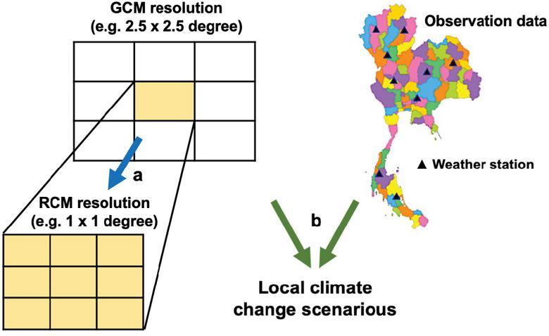
Figure 1 The concept of downscaling method. a (blue arrow) and b (green arrow) pathways are dynamical downscaling method and statistical downscaling method, respectively.
When comparing DD and SD methods for simulating climate change, the SD method model provided more unity of simulated results than DD method [40]. Although the accuracy from both methods is quite similar, the SD method has many advantages which overcome DD method, which is not only less time consuming but also suitable for regional and national level. Moreover, SD method can provide site-specific climate projections, while RCM cannot due to computational limitation of spatial resolution [18]. The relation between large-scale atmospheric characteristics (circulation, temperature, moisture, etc.) and observation data (temperature, precipitation, etc.) were collected to perform SD for local climate change scenarios as illustrated in Figure 1. This model is possible and reliable due to including observation data and producing small data for climate simulation. Thus, SD method has been used in this research for simulating Thailand climate change model.
This research demonstrates that local-scale climate projections obtained by means of SD method is sensitive to reanalysis used for calibration. Researchers applied the statistical downscaling model (SDSM) by the methods LR, GP, SVM, and DL.
Table 1 The pros and cons of each machine learning method
| Machine | ||
| Learning | ||
| Methods | Advantages | Disadvantages |
| Linear regression (LR) |
• Simple to perform [41] • Widely available software • Useful for linear simulate model |
• Unsuitable for non-linear • Risk of unnecessarily complicated analysis |
| Gaussian process (GP) |
• Extremely flexible • Powerful tool for nonparametric regression • Conceptually straightforward and easily accommodate prior knowledge • Requires fewer parameters to be fit than other methods [42] |
• Complex method • Lack of suitable software |
| Support vector machine (SVM) |
• Easy to control complexity non-linear data input • Overfitting problem is not as much as other methods |
• Computational expensive • Require the suitable kernel function |
| Deep learning (DL) |
• Easily identify complex relationships between dependent and independent variables [43], [44] • Suitable for classification/regression • Tolerate noisy data • Good prediction • Some tolerance to correlated inputs • Incorporating the predictive power of different input combinations |
• Not robust to outliers • Susceptible to irrelevant features • Difficult in dealing with big data with complex model |
2.1.1 Methods
The selected four machine learning methods of SD, used in this work, are LR, GP, SVM, and DL. The pros and cons of each machine learning method are shown in Table 1.
2.1.1.1 Linear regression
LR is the most basic type of regression and commonly used predictive analysis. One variable is considered to be an explanatory variable, and the other is considered to be a dependent variable. LR was the first type of regression analysis to be studied rigorously and to be used extensively in practical applications. This is because models which depend linearly on their unknown parameters are easier to fit than models which are non-linearly related to their parameters and because the statistical properties of the resulting estimators are easier to determine [41]. The simplest form of the equation with one dependent and one independent variable is defined by the formula
| (1) |
2.1.1.2 Gaussian process
GP is acceptable as stochastic process for the analysis of regression, classification, and decision in machine learning. GP can provide impressive performance in even low number of training data. A GP is fully specified by its mean function and covariance function . This is a natural generalization of the Gaussian distribution whose mean and covariance are a vector and matrix.
| (2) | |
| (3) |
A GP prior over functions can be thought of as a Gaussian prior on the coefficients where
| (4) |
In many interesting cases, .
We can choose ’s as eigenfunctions of the kernel wrt [45]
| (5) |
2.1.1.3 Deep learning
DL allows computational models that are composed of multiple processing layers to learn representations of data with multiple levels of abstraction. These methods have dramatically improved the state-of-the-art in speech recognition, visual object recognition, object detection, and many other domains such as drug discovery and genomics. DL discovers intricate structure in large data sets by using the backpropagation algorithm to indicate how a machine should change its internal parameters that are used to compute the representation in each layer from the representation in the previous layer [46]. Deep convolutional nets have brought about breakthroughs in processing images [47], video, speech and audio, whereas recurrent nets have shone light on sequential data such as text and speech.
In the context of artificial neural networks, the rectifier is an activation function defined as
| (6) |
where is the input to a neuron. This is also known as a ramp function and is analogous to half-wave rectification in electrical engineering. This activation function was first introduced to a dynamical network by Hahnloser et al. in a 2000 paper in Nature with strong biological motivations and mathematical justifications. It has been used in convolutional networks more effectively than the widely used logistic sigmoid (which is inspired by probability theory; see logistic regression) and its more practical counterpart, the hyperbolic tangent. The rectifier is, as of 2017, the most popular activation function for deep neural networks. A unit employing the rectifier is also called a rectified linear unit (ReLU).
2.1.1.4 Support vector machine
SVMs are a set of related supervised learning methods that are used in classification and regression analysis. The basic idea of the SVM for regression analysis is explained below.
Consider the finite training sample pattern , where is a sample value of the input vector consisting of training patterns (i.e., and is the corresponding value of the desired model output. A non-linear transformation function is defined to map the input space to a higher dimension feature space, . A non-linear relation between inputs and outputs in the original input space is shown in the following equation:
| (7) |
where is the actual model output, and and are adjustable coefficients model parameters. The objective function in SVMs task is
| (8) |
The constrained that may derive from dual Lagrangian is
| (9) |
The computation involve calculating transformed vector, the solution method called kernel trick. The mapping kernel can be defined as
| (10) |
The kernel trick is a method for calculating similarity in the transformed space using the original space, helps to address in mapping function by Mercer’s theorem, computing time using kernel function is cheaper than using the transformed attribute set, and avoids curse of dimensionality problem because the computations are performed in the original space.
Mercer’s theorem is a function to perform mapping of the attributes of the original space to the feature space.
| (11) |
A polynomial kernel mapping is a popular method for non-linear modeling.
| (12) | |
| (13) |
Radial basis function (RBF) kernel is used to map the input data into higher dimensional feature space, which is given by
| (14) |
where is the width of RBF kernel which can be adjusted to control the expressivity of RBF. The RBF kernels have localized and finite responses across the entire range of predictors.
The advantage with RBF kernel is that it non-linearly maps the training data into a possibly infinite dimensional space; thus, it can effectively handle the situations when the relationship between predictors and predictand is non-linear. Moreover, the RBF is computationally simple than polynomial kernel, which has more parameters [30, 48].
2.2 Study Area and Data
2.2.1 Global climate model
GCM, representing physical processes in the atmosphere, ocean, cryosphere and land surface, are numerical models that are the most advanced tools currently available for simulating response of the global climate system which has increase of greenhouse gas concentrations. There are simpler models than GCMs that are used to provide globally or regionally averaged estimates of the climate response, but only GCMs are possible in conjunction with nested regional models which have the potential to provide geographically and physically consistent estimates of regional climate change, which are required in impact analysis.
The global climate information has been provided by the complex mathematical model which is a GCM. The c changes which usually described by GCMs when different pressure, chemical composition, velocities and temperature that interact with each other. Some GCMs focused on modeling of the atmosphere are called atmosphere global circulation models (AGCMs). Additionally, the model of the ocean has also gained attention which is called OGCMs. Moreover, the advanced model that couple the atmosphere and ocean (AOGCMs) have been simulated; however, the calculation is more complex.
GCMs depict the climate using a three-dimensional grid over the globe (Figure 2), typically having a horizontal resolution of between 250 and 600 kilometers, 10 to 20 vertical layers in the atmosphere, and, sometimes, as many as 30 layers in the oceans. Their resolution is thus quite coarse relative to the scale of exposure units in most impact assessments. Moreover, many physical processes, such as those related to clouds, also occur at smaller scales and cannot be properly modeled. GCMs have gained attention from researcher which was developed by Community earth system model called Community Climate System Model (CCSM) [49].
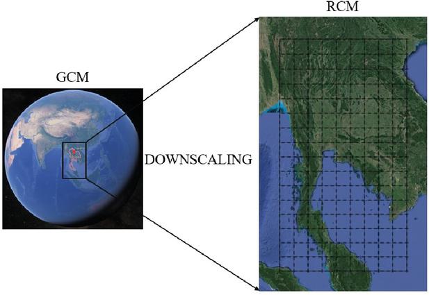
Figure 2 General circulation models.
2.2.2 National oceanic and atmospheric administration
National Oceanic and Atmospheric Administration (NOAA) is the U.S. Department of Commerce that provides data, tools, and information to help people understand and prepare for climate variability and change.
Table 2 The geographic coordinate of 45 weather stations in Thailand used in this study
| Station | Latitude | Longitude | Station | Latitude | Longitude | ||
| 1 | MAE HONG SON | 19.30 | 97.83 | 24 | PRACHIN BURI | 14.05 | 101.37 |
| 2 | CHIANG RAI | 19.88 | 99.83 | 25 | NAKHON RATCHASIMA | 14.97 | 102.08 |
| 3 | MAE SARIANG | 18.17 | 97.93 | 26 | SURIN | 14.88 | 103.50 |
| 4 | CHIANG MAI | 18.78 | 98.98 | 27 | KANCHANABURI | 14.02 | 99.53 |
| 5 | LAMPANG | 18.28 | 99.52 | 28 | BANGKOK METROPOLIS | 13.73 | 100.57 |
| 6 | PHRAE | 18.17 | 100.17 | 29 | DON MUANG | 13.92 | 100.60 |
| 7 | NAN | 18.77 | 100.77 | 30 | CHON BURI | 13.37 | 100.98 |
| 8 | UTTARADIT | 17.62 | 100.10 | 31 | ARANYAPRATHET | 13.70 | 102.58 |
| 9 | LOEI | 17.45 | 101.73 | 32 | HUA HIN | 12.58 | 99.95 |
| 10 | UDORN AB (USAF) | 17.38 | 102.80 | 33 | SATTAHIP | 12.68 | 100.98 |
| 11 | SAKON NAKHON | 17.15 | 104.13 | 34 | CHANTHABURI | 12.60 | 102.12 |
| 12 | NAKHON PHANOM | 17.42 | 104.78 | 35 | PRACHUAP KHIRI KHAN | 11.80 | 99.80 |
| 13 | MAE SOT | 16.67 | 98.55 | 36 | KHLONG YAI | 11.77 | 102.88 |
| 14 | TAK | 16.88 | 99.15 | 37 | CHUMPHON | 10.48 | 99.18 |
| 15 | PHITSANULOK/ SARIT | 16.82 | 100.27 | 38 | KO SAMUI | 9.47 | 100.05 |
| 16 | PHETCHABUN | 16.43 | 101.15 | 39 | SURAT THANI | 9.12 | 99.15 |
| 17 | KHON KAEN | 16.43 | 102.83 | 40 | NAKHON SI THAMMARAT | 8.53 | 99.95 |
| 18 | MUKDAHAN | 16.53 | 104.72 | 41 | PHUKET | 7.88 | 98.40 |
| 19 | NAKHON SAWAN | 15.80 | 100.17 | 42 | PHUKET AIRPORT | 8.13 | 98.32 |
| 20 | ROI ET | 16.05 | 103.68 | 43 | TRANG | 7.52 | 99.62 |
| 21 | UBON RATCHATHANI | 15.25 | 104.87 | 44 | SONGKHLA | 7.20 | 100.62 |
| 22 | SUPHAN BURI | 14.47 | 100.13 | 45 | HAT YAI | 6.92 | 100.43 |
| 23 | LOP BURI | 14.80 | 100.62 |
For this research, we used Global Historical Climatology Network (GHCN) data which is climate summaries from weather station across the globe. These data were proved and analyzed; thus, they can be used as adequate and reliable quality data for this research. GHCN data were archived from more than 20 sources, and some data sets have collected more than 175 years while others have promptly updated within 1 hour. Older NCEI-maintained data sets which are modeled for daily temporal resolution were replaced by official archived data set from GHCN.
In this research, daily weather data from up to 45 weather stations as illustrated in Table 2 of GHCN which covered all regions in Thailand were used as predictands to simulate with SD method including GCM as predictor.
3 Methodology
The Network Common Data Form (NetCDF) of GCMs from NOAA is a standard of climate change research. NetCDF is a matrix data which composes of three dimensions which are latitude, longitude, and time. The GCM data have collected which cover the longitude from 180.00 to 180.00 and latitude from 90.00 to 90.00 that across the globe in 1951–2005 [49]. In this research, latitude from 5 to 21 and longitude from 97 to 105 were selected as study area in Thailand. The values of maximum and minimum of temperature and precipitation from NetCDF were collected as matrix. These values were considered as predictors for SD calculation in this research. The predictands which also are values of maximum and minimum of temperature and precipitation were collected from 45 weather stations of GHCN in six regions of Thailand.
3.1 Statistical Downscaling Method
Machine learning methods were used to calculate the predictors and predictands together. Predictors which are maximum and minimum of temperature and precipitation were applied for constructing the model from each station. For each method, we choose all covariates from each variable, maximum temperature (TMAX), minimum temperature (TMIN), and precipitation, totaling 18,952 covariates. Analysis and evaluation of downscaled projections aim to capture daily anomalies for six regions in Thailand. The experiments were divided to four statistical method including DL, GP, LR, and SVM. Moreover, data set GCM from CCSM4 will be used in this research [49].
Table 3 Data set of GCM
| Experiment Number | Statistical Downscale Method | Number of Station | GCM Models |
| 1 | Deep learning | 45 | CCSM4 |
| 2 | Gaussian process | 45 | CCSM4 |
| 3 | Linear regression | 45 | CCSM4 |
| 4 | Support vector machine | 45 | CCSM4 |
The technical route of the research in this paper is described in Figure 3. In this work, each model for each TMAX, TMIN, and PRCP composed of TMAX, TMIN, and PRCP data from GCM were assigned as predictor. This kind of calculation generates new model which is more accurate and precise.
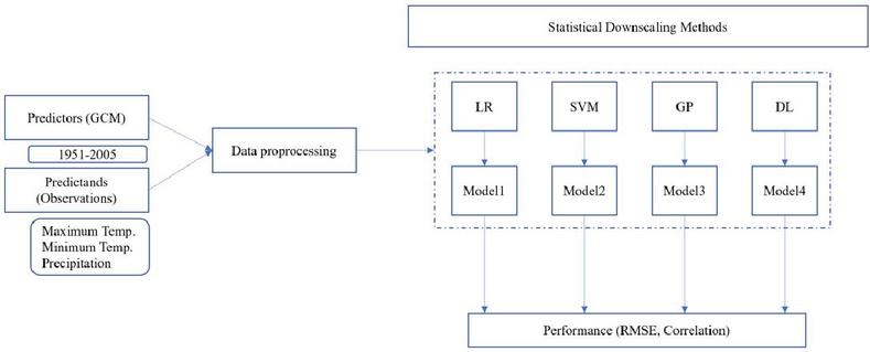
Figure 3 The technical route of this study.
Table 4 Kernel comparison of SVM
| Climate Variable | Kernel | RMSE | Rank |
| PRCP | Dot | 860.856 | 5 |
| PRCP | Epanechnikov | 106.380 | 4 |
| PRCP | Multiquadric | 100.297 | 1 |
| PRCP | Polynomial | 105.367 | 2 |
| PRCP | Radial | 106.133 | 3 |
| TMIN | Dot | 22.858 | 1 |
| TMIN | Epanechnikov | 46.109 | 5 |
| TMIN | Multiquadric | 42.324 | 3 |
| TMIN | Polynomial | 34.680 | 2 |
| TMIN | Radial | 46.100 | 4 |
| TMAX | Dot | 25.523 | 1 |
| TMAX | Epanechnikov | 33.151 | 4 |
| TMAX | Multiquadric | 32.978 | 3 |
| TMAX | Polynomial | 29.017 | 2 |
| TMAX | Radial | 33.153 | 5 |
Table 5 Kernel comparison of GP
| Climate Variable | Kernel | RMSE | Rank |
| PRCP | RBF | 105.386 | 2 |
| PRCP | Cauchy | 114.288 | 7 |
| PRCP | Epanechnikov | 106.749 | 3 |
| PRCP | Gaussian_combination | 106.749 | 4 |
| PRCP | Laplace | 108.519 | 6 |
| PRCP | Multiquadric | 99.551 | 1 |
| PRCP | Sigmoid | 106.749 | 5 |
| TMIN | RBF | 199.127 | 4 |
| TMIN | Cauchy | 31.096 | 1 |
| TMIN | Epanechnikov | 205.452 | 5 |
| TMIN | Gaussian_combination | 205.452 | 6 |
| TMIN | Laplace | 110.355 | 3 |
| TMIN | Multiquadric | 74.469 | 2 |
| TMIN | Sigmoid | 205.452 | 7 |
| TMAX | RBF | 328.217 | 4 |
| TMAX | Cauchy | 47.746 | 1 |
| TMAX | Epanechnikov | 329.238 | 5 |
| TMAX | Gaussian_combination | 329.238 | 6 |
| TMAX | Laplace | 199.881 | 2 |
| TMAX | Multiquadric | 208.369 | 3 |
| TMAX | Sigmoid | 329.238 | 7 |
The predictors and predictands from GCM and GHCN, respectively, were selected, and then prepared variables for further calculation by data processing. The data from Mae Hong Son station were selected for comparing the kernel. From Table 4, the calculated root mean square error (RMSE) was performed by five kernels from SVM: dot, Epanechnikov, multiquadric, polynomial, and radial. The results indicated that the polynomial (bold texts) provided the best performance as the lowest RMSE. Each kernel was rated by rank.
The first rank is the best performance due to the lowest RMSE. Then, rank of each climate variable was averaged. The top three of averaged rank are polynomial, multiquadric, and dot of 2.00, 2.33, and 2.33, respectively. Thus, polynomial will be used as kernel for further experiment. The seven kernels from GP were also compared as illustrated in Table 5. The results demonstrated that cauchy (bold texts) showed the best performance of GP although the averaged rank of cauchy is the second of 3.00. The first and third ranks are multiquadric of 2.00 and RBF of 3.33, respectively. However, from TMAX, the cauchy shows the lowest RMSE which is highly different from the multiquadric of the third rank. Therefore, cauchy will be selected as suitable kernel for further experiment in GP model.
4 Results and Discussion
The collected data from both GCMs and 45 weather stations were used for calculation of correlation and RMSE. The box plot was plotted by dividing into correlation and RMSE as illustrated in Figure 4. The results indicated that the DL provided the best performance as the highest correlation values of all climate values (PRCP, TMAX, and TMIN). The correlation PRCP obviously found that DL provides the highest value. LR and SVM provided correlation TMAX and TMIN which are quite high as DL. However, GP found that it is the lowest correlation value in all climate values due to unsuitability for this kind of parametric data and also provided high RMSE. The RMSEs of PRCP, TMAX, and TMIN found that DL, LR, and SVM offer quite similar values.

Figure 4 Box plot of correlation and RSME that compares between four SDs for (a) and (d) PRCP, (b) and (e), TMAX, and (c) and (f) TMIN.
Due to the geographical shape of Thailand, quite long latitude, the climate pattern highly changed along latitude. Thus, each model was applied to each region in Thailand for finding the suitable regional model. The experiment was divided into six regions of Thailand due to individual climate changes. The seasons in Thailand are rainy season from May to the middle of October (approximately five months), winter from the middle of November to the middle of February (approximately three months), and summer from February to May (approximately three months). The rainy season is obviously found in Northern, North East, Central, East, and South West coast. The cold weather is found in all regions of Thailand in the winter; however, in Southern, rarely cold weather is found. In addition, in the southern down from Surat Thani, often plenty of rain is found in winter which is considered as rainy season of south Thailand. In summer, the hottest weather period which is well-known in Thailand for even foreigners is in the middle of April. The change of weather from rainy season to winter from October to November was indicated as season change period.
In this study, using k-fold cross-validation, that is a resampling used to evaluate machine learning models. The researcher place of k is 10 so becoming 10-Fold cross-validation. The downscaling method based on LR, GP, SVM, and DL is set up and weighted average of precipitation, TMAX and TMIN sequences from 1951 to 2005, is simulated. And the correlation and RMSE of the 45 stations are calculated. The compared values are shown in Tables 6 and 7.
Table 6 The results of correlation by different methods for PRCP, TMAX, and TMIN based on six regions in Thailand (N: North, NE: North East, CE: Central, E: East, W: West and S: South).
| Climate Variable | Correlation | ||||||
| N | NE | CE | E | W | S | ||
| PRCP | DL | 0.35 | 0.35 | 0.32 | 0.36 | 0.29 | 0.27 |
| GP | 0.10 | 0.10 | 0.06 | 0.09 | 0.07 | 0.05 | |
| LR | 0.24 | 0.24 | 0.21 | 0.25 | 0.20 | 0.19 | |
| SVM | 0.10 | 0.09 | 0.06 | 0.10 | 0.06 | 0.12 | |
| TMAX | DL | 0.69 | 0.62 | 0.64 | 0.49 | 0.66 | 0.62 |
| GP | 0.22 | 0.21 | 0.16 | 0.04 | 0.21 | 0.15 | |
| LR | 0.63 | 0.56 | 0.58 | 0.44 | 0.61 | 0.61 | |
| SVM | 0.59 | 0.53 | 0.54 | 0.38 | 0.58 | 0.57 | |
| TMIN | DL | 0.84 | 0.78 | 0.72 | 0.66 | 0.75 | 0.47 |
| GP | 0.71 | 0.62 | 0.48 | 0.37 | 0.51 | 0.19 | |
| LR | 0.85 | 0.80 | 0.74 | 0.69 | 0.78 | 0.53 | |
| SVM | 0.84 | 0.81 | 0.79 | 0.78 | 0.80 | 0.74 | |
Table 7 The results of RMSE by different methods for PRCP, TMAX, and TMIN based on six regions in Thailand (N: North, NE: North East, CE: Central, E: East, W: West and S: South).
| Climate Variable | RMSE | ||||||
| N | NE | CE | E | W | S | ||
| PRCP | DL | 94.46 | 112.93 | 102.50 | 144.85 | 101.05 | 148.48 |
| GP | 105.45 | 125.76 | 112.32 | 166.20 | 108.98 | 163.08 | |
| LR | 97.32 | 116.71 | 105.17 | 150.23 | 102.69 | 150.44 | |
| SVM | 105.92 | 126.57 | 112.87 | 165.71 | 109.27 | 203.61 | |
| TMAX | DL | 23.19 | 25.27 | 20.72 | 18.15 | 20.96 | 19.62 |
| GP | 47.79 | 47.73 | 47.19 | 45.29 | 46.11 | 44.51 | |
| LR | 24.81 | 26.43 | 21.86 | 18.47 | 22.21 | 17.68 | |
| SVM | 25.92 | 27.12 | 22.61 | 19.04 | 23.08 | 18.61 | |
| TMIN | DL | 24.84 | 25.24 | 21.33 | 18.25 | 20.61 | 12.35 |
| GP | 32.19 | 34.54 | 34.22 | 33.71 | 33.29 | 33.18 | |
| LR | 21.99 | 23.07 | 19.66 | 16.79 | 18.66 | 11.40 | |
| SVM | 24.35 | 25.00 | 23.92 | 23.46 | 23.96 | 21.42 | |
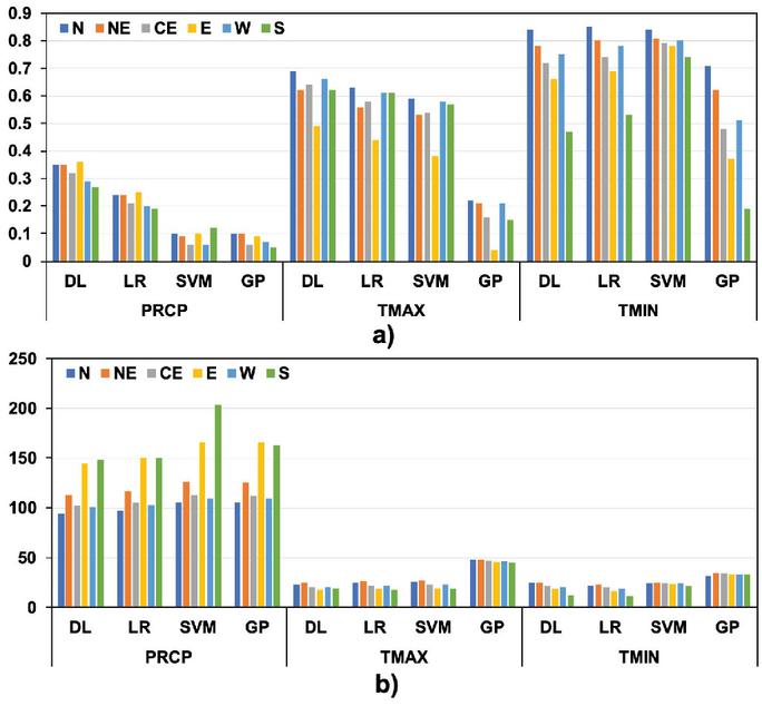
Figure 5 The results of (a) correlation and (b) RMSE by different methods for PRCP, TMAX, and TMIN based on six regions in Thailand (N: North, NE: North East, CE: Central East, E: East, W: West and S: South).
Figure 5 illustrates the correlation precipitation. The results indicated that DL provides the best correlation for precipitation calculation owing to process of finding relationships between variables. GP, LR, and SVM provide lower value of correlation precipitation as illustrated in Figure 5(a). The correlation TMAX and TMIN, the results from LR, and SVM were found to be quite similar, while DL provides better results as the highest among all models. The GP still provided the lowest accuracy due to parametric data.

Figure 6 The correlation and RMSE mapping of Thailand for different models (DL, GP, LR, and SVM).
In Figure 5(b), the results of RMSE PRCP indicated that the performance of DL is obviously better than the others being the lowest RMSE. However, the results of RMSE TMAX and TMIN of LR and SVM demonstrated that the performance is quite similar to DL.
The mappings of correlation and RMSE were generated for investigating results in station level as shown in Figure 6. The results demonstrated that some region has huge data distribution such as PRCP in South region. As South region located between Andaman Sea and Gulf of Thailand, it leads to high variation of rain. Both banks of South found quite similar calculated climate variables; however, Gulf of Thailand bank provided a worse result due to higher variation of rain level. TMAX and TMIN illustrated that data distributions from calculation are quite similar in each region. However, North East region is a huge region which lengthily covers along longitude that affects more temperature different than other regions. In East region, PRCP found low correlation for all machine learning methods due to high variance from Gulf of Thailand and neighboring countries. Nevertheless, TMAX and TMIN still provided high performance of calculation as well as other regions.
Figure 5 demonstrated that GP performance provides the lowest RMSE and poor correlation with both TMAX and TMIN in all regions. Moreover, DL notably provided good performance as high correlation and low RMSE for overall regions. Due to stable temperature in South, calculated TMAX and TMIN obviously demonstrated better correlation and RMSE for all models.
In this study, one GCM data set and 45 weather stations were used for calculation. However, more GCM data set can offer more accuracy and ability for investigating SD. Although more data sets are required for improving accuracy, the present results have led us to believe that our approach will be a powerful tool that offers a new strategy for researchers to discover further models.
The climate projection has gained attention and was developed by GCMs. However, the local climate projection still requires improvement due to small scale and fine resolution. SD and DD are two methods for GCM downscaling model. SD, using GCMs data and data set from weather stations and focusing on the statistical distribution characteristics, was used in this work for climate variable analysis in Thailand. Additionally, SD has a number of advantages that overcome DD such as less time consumption, uncomplicated method, and fine scale calculation. The models for SD that performed in this study are DL, GP, LR, and SVM. As expected, the results indicated that DL provided the highest performance and accuracy. Although the result of the DD for the PRCP quite similar to the others model that because the inconsistent data set such as region with randomness of precipitation. Although some climate variables achieved from LR and SVM are quite similar to DL, calculation time of DL found that less than LR and SVM approximately 10-fold. Therefore, SD is suitable for this kind of analytical data set and should be improved at comprehensive analysis to get better performance and accuracy.
5 Conclusion
The ability of SD methods to produce credible results is necessary for a research. Many researches have studied SD; however, no researches summarized which the best performance model is. Each SD model is suitable for different data sets; in this research, the comparison of four SDs, i.e., DL, GP, LP, and SVM, was done. The results indicated that DL, a popular approach of SD, was found to show the best performance in all calculations (PRCP, TMAX, and TMIN). Result of the PRCP from North and North East, which is rarely found rain, leads to the result of PRCP is better than other regions. In contrast, PRCP from South, which often found storm in the entire year, then, provided unsuitable model for calculation. Calculated TMAX and TMIN in North and South demonstrated poor and good performance for all models, respectively. Due to high variable temperature in North, the calculated TMAX and TMIN provided low correlation and high RMSE. On the other hand, calculated TMAX and TMIN found high correlation and low RMSE owing to stable temperature in South. From the presented results, the suitable model for each region can be selected for future GCMs. Moreover, the suitable model will be consistent with suitable and desired weather station. Thus, future climate prediction can be forecasted and applied to future application. We believe that this study paves the way for future climate change prediction with reliable model and excellent performance.
References
[1] Lidskog, R. and D. Sjödin, Extreme events and climate change: the post-disaster dynamics of forest fires and forest storms in Sweden. Scandinavian Journal of Forest Research, 2016. 31(2): p. 148–155.
[2] IPCC, AR5: Climate Change, Synthesis Report. 2014.
[3] Pachauri, R.K. and L.A.M. (eds.), Climate Change 2014: Synthesis Report. Contribution of Working Groups I, II and III to the Fifth Assessment Report of the Intergovernmental Panel on Climate Change. IPCC, Geneva, Switzerland, 2014: p. 151.
[4] Trzaska, S. and E. Schnarr, A Review of Downscaling Methods for Climate Change Projections. 2014.
[5] Piao, S., P. Ciais, Y. Huang, Z. Shen, S. Peng, J. Li, L. Zhou, H. Liu, Y. Ma, Y. Ding, P. Friedlingstein, C. Liu, K. Tan, Y. Yu, T. Zhang, and J. Fang, The impacts of climate change on water resources and agriculture in China. Nature, 2010. 467(7311): p. 43–51.
[6] Sa, J.C., R. Lal, C.C. Cerri, K. Lorenz, M. Hungria, and P.C. de Faccio Carvalho, Low-carbon agriculture in South America to mitigate global climate change and advance food security. Environ Int, 2017. 98: p. 102–112.
[7] Van Passel, S., E. Massetti, and R. Mendelsohn, A Ricardian Analysis of the Impact of Climate Change on European Agriculture. Environmental and Resource Economics, 2016. 67(4): p. 725–760.
[8] Barrett, B., J.W. Charles, and J.L. Temte, Climate change, human health, and epidemiological transition. Preventive Medicine, 2015. 70: p. 69–75.
[9] McMichael, A.J., R.E. Woodruff, and S. Hales, Climate change and human health: present and future risks. The Lancet, 2006. 367(9513): p. 859–869.
[10] Mourato, S., M. Moreira, and J. Corte-Real, Water Resources Impact Assessment Under Climate Change Scenarios in Mediterranean Watersheds. Water Resources Management, 2015. 29(7): p. 2377–2391.
[11] Sowers, J., A. Vengosh, and E. Weinthal, Climate change, water resources, and the politics of adaptation in the Middle East and North Africa. Climatic Change, 2011. 104(3): p. 599–627.
[12] Maraun, D., F. Wetterhall, A.M. Ireson, R.E. Chandler, E.J. Kendon, M. Widmann, S. Brienen, H.W. Rust, T. Sauter, M. Themeßl, V.K.C. Venema, K.P. Chun, C.M. Goodess, R.G. Jones, C. Onof, M. Vrac, and I. Thiele-Eich, Precipitation downscaling under climate change: Recent developments to bridge the gap between dynamical models and the end user. Reviews of Geophysics, 2010. 48(3).
[13] Delworth, T.L., A.J. Broccoli, A. Rosati, R.J. Stouffer, V. Balaji, J.A. Beesley, W.F. Cooke, K.W. Dixon, J. Dunne, K.A. Dunne, J.W. Durachta, K.L. Findell, P. Ginoux, A. Gnanadesikan, C.T. Gordon, S.M. Griffies, R. Gudgel, M.J. Harrison, I.M. Held, R.S. Hemler, L.W. Horowitz, S.A. Klein, T.R. Knutson, P.J. Kushner, A.R. Langenhorst, H.-C. Lee, S.-J. Lin, J. Lu, S.L. Malyshev, P.C.D. Milly, V. Ramaswamy, J. Russell, M.D. Schwarzkopf, E. Shevliakova, J.J. Sirutis, M.J. Spelman, W.F. Stern, M. Winton, A.T. Wittenberg, B. Wyman, F. Zeng, and R. Zhang, GFDL’s CM2 Global Coupled Climate Models. Part I: Formulation and Simulation Characteristics. Journal of Climate, 2006. 19(5): p. 643–674.
[14] Delworth, T.L., A. Rosati, W. Anderson, A.J. Adcroft, V. Balaji, R. Benson, K. Dixon, S.M. Griffies, H.-C. Lee, R.C. Pacanowski, G.A. Vecchi, A.T. Wittenberg, F. Zeng, and R. Zhang, Simulated Climate and Climate Change in the GFDL CM2.5 High-Resolution Coupled Climate Model. Journal of Climate, 2012. 25(8): p. 2755–2781.
[15] Chou, S.C., J.A. Marengo, A.A. Lyra, G. Sueiro, J.F. Pesquero, L.M. Alves, G. Kay, R. Betts, D.J. Chagas, J.L. Gomes, J.F. Bustamante, and P. Tavares, Downscaling of South America present climate driven by 4-member HadCM3 runs. Climate Dynamics, 2012. 38(3): p. 635–653.
[16] Roeckner, E., K. Arpe, L. Bengtsson, S. Brinkop, L. Duemenil, M. Esch, E. Kirk, F. Lunkeit, M. Ponater, B. Rockel, R. Sausen, U. Schleese, S.D. Schubert, and M. Windelband. Simulation of the present-day climate with the ECHAM model: Impact of model physics and resolution. 1992.
[17] Molteni, F., R. Buizza, T.N. Palmer, and T. Petroliagis, The ECMWF Ensemble Prediction System: Methodology and validation. Quarterly Journal of the Royal Meteorological Society, 1996. 122(529): p. 73–119.
[18] Sylwia Trzaska, E., A Review of Downscaling Methods for Climate Change Projections. 2014.
[19] Haines, A., R.S. Kovats, D. Campbell-Lendrum, and C. Corvalan, Climate change and human health: impacts, vulnerability and public health. Public Health, 2006. 120(7): p. 585–96.
[20] Jakob Themeßl, M., A. Gobiet, and A. Leuprecht, Empirical-statistical downscaling and error correction of daily precipitation from regional climate models. International Journal of Climatology, 2011. 31(10): p. 1530–1544.
[21] Dixon, K.W., J.R. Lanzante, M.J. Nath, K. Hayhoe, A. Stoner, A. Radhakrishnan, V. Balaji, and C.F. Gaitán, Evaluating the stationarity assumption in statistically downscaled climate projections: is past performance an indicator of future results? Climatic Change, 2016. 135(3-4): p. 395–408.
[22] Kalogirou, S.A., S. Pashiardis, and A. Pashiardi, Statistical analysis and inter-comparison of the global solar radiation at two sites in Cyprus. Renewable Energy, 2017. 101: p. 1102–1123.
[23] Boé, J., L. Terray, F. Habets, and E. Martin, Statistical and dynamical downscaling of the Seine basin climate for hydro-meteorological studies. International Journal of Climatology, 2007. 27(12): p. 1643–1655.
[24] Manzanas, R., S. Brands, D. San-Martín, A. Lucero, C. Limbo, and J.M. Gutiérrez, Statistical Downscaling in the Tropics Can Be Sensitive to Reanalysis Choice: A Case Study for Precipitation in the Philippines. Journal of Climate, 2015. 28(10): p. 4171–4184.
[25] Tatli, H., H. Nüzhet Dalfes, and M. Sibel, A statistical downscaling method for monthly total precipitation over Turkey. International Journal of Climatology, 2004. 24(2): p. 161–180.
[26] Tajbakhsh, N. and K. Suzuki, Comparing two classes of end-to-end machine-learning models in lung nodule detection and classification: MTANNs vs. CNNs. Pattern Recognition, 2017. 63: p. 476–486.
[27] Sunyer, M.A., H. Madsen, and P.H. Ang, A comparison of different regional climate models and statistical downscaling methods for extreme rainfall estimation under climate change. Atmospheric Research, 2012. 103: p. 119–128.
[28] Campozano, L., D. Tenelanda, E. Sanchez, E. Samaniego, and J. Feyen, Comparison of Statistical Downscaling Methods for Monthly Total Precipitation: Case Study for the Paute River Basin in Southern Ecuador. Advances in Meteorology, 2016. 2016: p. 1–13.
[29] Abatzoglou, J.T. and T.J. Brown, A comparison of statistical downscaling methods suited for wildfire applications. International Journal of Climatology, 2012. 32(5): p. 772–780.
[30] Liu, J., D. Yuan, L. Zhang, X. Zou, and X. Song, Comparison of Three Statistical Downscaling Methods and Ensemble Downscaling Method Based on Bayesian Model Averaging in Upper Hanjiang River Basin, China. Advances in Meteorology, 2016. 2016: p. 1–12.
[31] Jeong, D.I., A. St-Hilaire, T.B.M.J. Ouarda, and P. Gachon, Comparison of transfer functions in statistical downscaling models for daily temperature and precipitation over Canada. Stochastic Environmental Research and Risk Assessment, 2011. 26(5): p. 633–653.
[32] Hewitson, B.C. and R.G. Crane, Consensus between GCM climate change projections with empirical downscaling: precipitation downscaling over South Africa. International Journal of Climatology, 2006. 26(10): p. 1315–1337.
[33] Chu, J.T., J. Xia, C.Y. Xu, and V.P. Singh, Statistical downscaling of daily mean temperature, pan evaporation and precipitation for climate change scenarios in Haihe River, China. Theoretical and Applied Climatology, 2009. 99(1–2): p. 149–161.
[34] Chen, S.-T., P.-S. Yu, and Y.-H. Tang, Statistical downscaling of daily precipitation using support vector machines and multivariate analysis. Journal of Hydrology, 2010. 385(1–4): p. 13–22.
[35] Fealy, R. and J. Sweeney, Statistical downscaling of precipitation for a selection of sites in Ireland employing a generalised linear modelling approach. International Journal of Climatology, 2007. 27(15): p. 2083–2094.
[36] Vu, M.T., T. Aribarg, S. Supratid, S.V. Raghavan, and S.-Y. Liong, Statistical downscaling rainfall using artificial neural network: significantly wetter Bangkok? Theoretical and Applied Climatology, 2015. 126(3–4): p. 453–467.
[37] Mendoza, P.A., B. Rajagopalan, M.P. Clark, K. Ikeda, and R.M. Rasmussen, Statistical Postprocessing of High-Resolution Regional Climate Model Output. Monthly Weather Review, 2015. 143(5): p. 1533–1553.
[38] Hadipour, S., S. Harun, A. Arefnia, and M. Alamgir, Transfer Function Models for Statistical Downscaling of Monthly Precipitation. Jurnal Teknologi, 2016. 78(9–4).
[39] Smid, M. and A.C. Costa, Climate projections and downscaling techniques: a discussion for impact studies in urban systems. International Journal of Urban Sciences, 2017. 22(3): p. 277–307.
[40] Gutiérrez, J.M., D. San-Martín, S. Brands, R. Manzanas, and S. Herrera, Reassessing Statistical Downscaling Techniques for Their Robust Application under Climate Change Conditions. Journal of Climate, 2013. 26(1): p. 171–188.
[41] Schneider, A., G. Hommel, and M. Blettner, Linear regression analysis: part 14 of a series on evaluation of scientific publications. Deutsches Arzteblatt international, 2010. 107(44): p. 776–782.
[42] Rasmussen, C.E., Gaussian Processes in Machine Learning, in Advanced Lectures on Machine Learning: ML Summer Schools 2003, Canberra, Australia, February 2 – 14, 2003, Tübingen, Germany, August 4 – 16, 2003, Revised Lectures, O. Bousquet, U. von Luxburg, and G. Rätsch, Editors. 2004, Springer Berlin Heidelberg: Berlin, Heidelberg. p. 63–71.
[43] LeCun, Y., Y. Bengio, and G. Hinton, Deep learning. Nature, 2015. 521(7553): p. 436–44.
[44] Schmidhuber, J., Deep learning in neural networks: an overview. Neural Netw, 2015. 61: p. 85–117.
[45] Girolami, M., Mercer kernel-based clustering in feature space. IEEE Transactions on Neural Networks, 2002. 13(3): p. 780–784.
[46] Tu, J.V., Advantages and disadvantages of using artificial neural networks versus logistic regression for predicting medical outcomes. Journal of Clinical Epidemiology, 1996. 49(11): p. 1225–1231.
[47] Sun, Y., X. Wang, and X. Tang, Deep Learning Face Representation by Joint Identification-Verification. Proc. NIPS, 2014. 27.
[48] Dibike, Y.B. and P. Coulibaly, Temporal neural networks for downscaling climate variability and extremes. Neural Networks, 2006. 19(2): p. 135–144.
[49] Gent, P.R., G. Danabasoglu, L.J. Donner, M.M. Holland, E.C. Hunke, S.R. Jayne, D.M. Lawrence, R.B. Neale, P.J. Rasch, M. Vertenstein, P.H. Worley, Z.-L. Yang, and M. Zhang, The Community Climate System Model Version 4. Journal of Climate, 2011. 24(19): p. 4973–4991.
Biographies

Kanawut Chattrairat is a Ph.D. student at IT Management Division, Faculty of Engineering, Mahidol University, Bangkok, Thailand. He received a B.Eng in Computer Engineering and a M.Sci. in Technology of Information Management. His research interests in Machine learning and Data processing. He is a software engineer with extensive experience and management skills and works for Financial Services Technology company. The company provides payment and banking solutions for the Bank around the glove.

Waranyu Wongseree received the B.E., M.E., and Ph.D. degrees in electrical engineering from the King Mongkut’s University of Technology North Bangkok, Bangkok, Thailand. His research interests include applied machine learning, climate model, bioinformatics, and home energy monitoring.

Adisorn Leelasantitham received the B.Eng. in Electronics and Telecommunications and M. Eng. in Electrical Engineering from King Mongkut’s University of Technology Thonburi (KMUTT), Thailand, in 1997 and 1999, respectively. He received his PhD degree in Electrical Engineering from Sirindhorn International Institute of Technology (SIIT), Thammasat University, Thailand, in 2005. He is currently the Associate Professor in Technology of Information System Management Program, Faculty of Engineering, Mahidol University, Thailand. His research interests include Applications of Blockchain Technology and Cryptocurrency, e.g. electricity trading platform, etc.,conceptual models for IT managements, image processing, AI, neural networks, machine learning, IoT platforms, data analytics, chaos systems and healthcare IT. He is a member of the IEEE.
Journal of Web Engineering, Vol. 20_5, 1397–1424.
doi: 10.13052/jwe1540-9589.2057
© 2021 River Publishers