An Optimized Algorithm to Construct QC-LDPC Matrix in Compressed Sensing

Xiaoqi Yin^{1, 2}, Jiansheng Qian^{1, *}, Xingge Guo¹ and Guohua Lin²

¹School of Informatiom and Electrical Engineering, China University of Mining and Technology, Xuzhou Jiangsu 221008, China

²Jiangsu Laboratory of Lake Environment Remote Sensing Technologies, Huaiyin Institute of Technology, Huaian Jiangsu 223003, China

E-mail: hy_xuebao2009@126.com

*Corresponding Author

Received 11 August 2020; Accepted 25 September 2020; Publication 16 December 2020

Abstract

Aiming at the problems such as the large amount of data in transmission and difficulties in hardware implementation, an optimized algorithm is put forward to generate QC-LDPC measurement matrix based on limited geometry in compressed sensing, which can eliminate the short girth of 4 in Tanner graph through the design of basis matrix. Because of the quasi-cyclic characteristics, it can be realized by shift register so as to reduce the complexity of coding. The simulation results indicate that QC-LDPC matrix is superior to traditional measurement matrices by using the same OMP algorithm, and there are good improvements in the aspects of PSNR, SSIM, NMSE and runtime, which are conductive to the application of compressed sensing theory in real-time data transmission.

Keywords: Measurement matrix, LDPC, quasi-cyclic, finite geometry, short girth, compressed sensing.

1 Introduction

The compressed sensing theory breaks the traditional sampling limitation and realizes the change of signal sampling, that is, only a small amount of sampling data can keep the information of the original signal, and the original signal can also be reconstructed accurately through these sampled data [1].

In the process of compressed sensing, signal recovery is a linear programming problem. Since the number of samples is much less than the length of the original signal, the linear programming problem is that the number of equations is less than the number of solutions, which are theoretically innumerable [2]. Based on these problems, Candes proposed the famous restricted isometry property (RIP) criterion in 2006, which provides sufficient conditions for the existence of the determined solutions of the underdetermined equations. However, it is not practical to use RIP criterion to construct the measurement matrix due to the high complexity. The basis for constructing the measurement matrix is to consider whether the matrix can satisfy the correlation property or RIP criterion with high probability [3].

At present, the measurement matrices can be divided into three categories as follows:

1. Randomly generated matrix, such as gauss random matrix, Bernoulli random matrix, etc., the elements of which are independently subject to a particular distribution and satisfy $m=O(k\log (n/k))$ [4].

2. Generated by transformation of orthogonal matrix, such as Fourier matrix, part Hadamard matrix, etc., which has a fast transformation algorithm, and its common feature is to select $m$ rows from an $n\times n$ orthogonal matrix randomly, and carry out normalization on the new matrix [5].

3. Generated by binary matrix, such as toplitz matrix and random sparse matrix, which is characterized by fixed construction mode [6].

The above matrix is not simple enough, the so-called simple refers to the matrix is highly sparse and its element is binarization. The theoretical measurement matrix is not actual to be implemented in hardware. In order to make it be applied to our real life more generally, the research should focus on the following problems:

(1) Sparsity
In the existing measurement matrix, such as random gaussian matrix, whose most orthogonal vector elements are not relevant [7], the sparse signal can be reconstructed from the measured values for high probability when it meets RIP criterion, but it has large density, which would lead to large amount of calculation in the process of recovery and cost more time, at the same time it would take up a lot of storage space, thus is not conducive to practical application [8].

(2) Hardware implementation
The hardware implementation of measurement matrix is also an important aspect of compressed sensing theory. The random matrix has a strong randomness in structure, that makes it hard to be realized in hardware [9]. On the other hand, the cyclic characteristics of toplitz matrix and cyclic matrix are easy for hardware implemention, but their effect in compressed sensing are relatively poor.

(3) Irrelevance
The measurement matrix should also meet the strict RIP criterion or irrelevancy, and have strong orthogonality [10]. Therefore, people prefer to the matrix with small computational load and easy to be implemented in hardware as the measurement matrix, so that the recovered signal can be better.

In recent years, low-density-parity-check (LDPC) codes have been applied to the signal recovery in compressed sensing theory. Due to the high sparsity of LDPC matrix, it is conducive to hardware implementation. As a measurement matrix, it has the advantages of binarity, high sparsity and good orthotropy [11]. But it should be noted that the girth of 4 should be avoided in the LDPC matrix. If it is in the matrix, the correlation between the two columns is increased, which is not conducive to the signal sampling. For these problems, it is proposed an improved method to generate quasi-cyslic low-density-parity-check (QC-LDPC) codes measurement matrix which is constructed in finite geometry. Based on the optimal design of the basis matrix, some short girths of QC-LDPC codes can be eliminated, and the decoding threshold can be improved, so that the performance of QC-LDPC codes can be optimized. The complexity of the construction process is low, and it has the characteristics of quasi-cyclic, which can not only save the storage space of the check matrix, but also reduce the complexity of coding and decoding so as to be suitable for the design of integrated circuits. At the same time, the coding process can be realized by shift register, which can greatly save the cost and be in line with the requirements of application.

2 Methodology and Related Works

2.1 Compressed Sensing of Signals

Let ${\{{\psi }_i\}}_{i=1}^N$ is a basis of $N$ dimensional real vector space ${\mathrm{R}}^N$, then for any dimension signal $x\in {\mathrm{R}}^{N\times 1}$, there is a set of coefficients ${\{x_i\}}_{i=1}^N$ that:

$$x=\sum _{i=1}^N{x}_i{\psi }_i=\mathrm{\Psi }\theta$$

(1)

Here, $\mathrm{\Psi }=({\psi }_1,{\psi }_2,\mathrm{\cdots },{\psi }_N)\in {\mathrm{R}}^{N\times N}$, $\theta ={({\theta }_1,{\theta }_2,\mathrm{\cdots },{\theta }_N)}^T$, ${\theta }_i=⟨x,{\psi }_i⟩$.

Definition 1: For the signal $x={(x_1,x_2,\mathrm{\dots },x_n)}^T\in {\mathrm{R}}^N$, if there is a group of basis $\mathrm{\Psi }$, which can get $x=\mathrm{\Psi }\theta$, there are $k$ non-zero component at most, and $k<N$, namely,

$${\parallel \theta \parallel }_0\le k$$

(2)

then $\theta$ is called a k-sparse signal.

Definition 2: For the signal $x={(x_1,x_2,\mathrm{\dots },x_n)}^T\in {\mathrm{R}}^N$, if a basis $\mathrm{\Psi }$ satisfies $x=\mathrm{\Psi }\theta$, and most components of $\theta$ are close to 0, then $x$ is called a compressible signal.

Definition 3: For a vector $\theta ={({\theta }_1,{\theta }_2,\mathrm{\dots },{\theta }_N)}^T\in {\mathrm{R}}^N$, the components of an N-dimensional vector ${\theta }^{\prime }\in {\mathrm{R}}^N$ are the same as $\theta$ in the $k$ positions with the largest amplitude, and zeros in the other positions, it is defined ${\theta }^{\prime }$ the optimal $k$ term approximation.

The measurement matrix $\mathrm{\Phi }$ is represented as $\mathrm{\Phi }=({\varphi }_1,{\varphi }_2,\mathrm{\dots },{\varphi }_{\mathrm{N}})$, and ${\varphi }_k={({\phi }_{1,k},{\phi }_{2,k},\mathrm{\dots },{\phi }_{N,k})}^T$, $k=1,2,\mathrm{\dots },N$, so the measurement vector y can be expressed as

$$y=\mathrm{\Phi }x=\mathrm{\Phi }\mathrm{\Psi }\theta =\mathrm{\Theta }\theta$$

(3)

where $\mathrm{\Theta }$ is the compressed sensing matrix whose row $M$ is far less than column $N$ when it meets the RIP criterion.

The non-correlation between $\mathrm{\Psi }$and $\mathrm{\Phi }$ is represented as

$$\mu (\mathrm{\Phi },\mathrm{\Psi })=\sqrt{N}\underset{1\le k,j\le N}{\max }|⟨{\varphi }_k,{\psi }_j⟩|$$

(4)

The range is $1\le \mu (\mathrm{\Phi },\mathrm{\Psi })\le \sqrt{N}$. For certain $\mathrm{\Psi }$, ${\mathrm{\Phi }}^{*}$ is the optimal measurement matrix when it can obtain the smallest value of $\mu (\mathrm{\Phi },\mathrm{\Psi })$. Therefore, there exists

$$\mu ({\mathrm{\Phi }}^{*},\mathrm{\Psi })=\min \left\{\sqrt{N}\underset{1\le k,j\le N}{\max }|⟨{\varphi }_k,{\psi }_j⟩|\right\}$$

(5)

where $\mathrm{\Phi }$ should satisfy ${\mathrm{\Phi }}^T\mathrm{\Phi }=I$.

2.2 LDPC Codes

The LDPC codes are often called the Gallager codes or the regular LDPC codes which refers to the linear block codes on a binary field. In the check matrix of the codes, each column has $\lambda$ non-zero elements, and each row has $\rho$ non-zero elements, that is, each bit in the codes participates in $\lambda$ check constraint, and each check constraint involves $\rho$ bits. $\rho$ and $\lambda$ are much less than the number of rows $M$ and columes $N$ respectively, that is, it is a sparse matrix.

LDPC codes can be graphically represented as Tanner graph. Regular LDPC codes (6,2,3) is shown in Figure 1. In the figure, there are variable nodes $\{v_1,v_2,\mathrm{\dots },v_6\}$ and check nodes $\{c_1,c_2,c_3,c_4\}$ with attachments between the two sets, but none insides them.

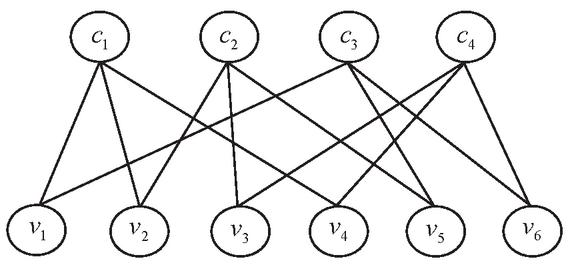
Figure 1 Tanner graph of LDPC codes (6,2,3).

There are many closed loops in the Tanner graph of LDPC codes, among which the shortest loop is called the girth. In the Tanner graph of the above example, the girth is 6. The girth size and closed loop distribution would effect the performance of LDPC codes to a large degree.

Given the check matrix of the regular codes $(\lambda ,\rho )$, if the rows are linearly independent, the code rate is $1-\lambda /\rho$. Otherwise, the code rate is greater than $1-\lambda /\rho$. Namely, the minimum code rate of regular LDPC code is:

$$R=(N-M)/N=1-\lambda /\rho$$

(6)

For regular LDPC codes, the average values of row weight and column weight of the check matrix remain unchanged, so the number of “1” in the check matrix is $\lambda \cdot N$. It increases linearly with the code length, while the elements of the check matrix grow as a square. Therefore, the check matrix is a very sparse matrix when the code length is very long [12]. Gallager demonstrated that regular codes had good hamming distance characteristics when $\lambda \ge 3$. The regular LDPC code is usually represented by $(N,\lambda ,\rho )$, where $N$ represents the code length, $\lambda$ represents the column weight, and $\rho$ represents the row weight.

For irregular LDPC codes, the number of “1” in each row and column of the check matrix are not exactly the same, correspondingly, the degrees of each variable nodes and check nodes in the Tanner graph are also not same. The edge of the degree distribution is usually expressed in sequence $\{{\lambda }_1,{\lambda }_2,\mathrm{\dots }{\lambda }_{d_l}\}$ and $\{{\rho }_1,{\rho }_2,\mathrm{\dots }{\rho }_{d_r}\}$, among them, ${\lambda }_i$ represents the ratio of the number of edges which are connected to variable nodes with degree $i$ to the number of total edges, ${\rho }_j$ represents the ratio of number of edges connected to check nodes with degree $j$ to the number of total edges, $d_l$ and $d_r$ represent the biggest degrees of variable nodes and check nodes respectively, so we can get

$$\sum _{i=1}^{d_l}{\lambda }_i=1,\sum _{j=1}^{d_r}{\rho }_j=1$$

(7)

The degree distribution sequence of edges can be expressed by polynomials as followers

$$\lambda (x)=\sum _{i=1}^{d_l}{\lambda }_i{x}^{i-1},\rho (x)=\sum _{j=1}^{d_r}{\rho }_j{x}^{j-1}$$

(8)

where $\lambda (1)={\sum }_{i=1}^{d_l}{\lambda }_i=1$, and $\rho (1)={\sum }_{j=1}^{d_r}{\rho }_j=1$.

Let the total number of edges in the Tanner diagram corresponding to an LDPC code be $E$, according to the degree distribution polynomial of the edges, the number of variable nodes with degree $i$ is $v_i=E{\lambda }_i/i$, and the number of check nodes with degree $j$ is $c_j=E{\rho }_j/j$, then the total number of variable nodes and check nodes are respectively given by

$n$	$={\displaystyle \sum _{i=1}^{d_l}}{v}_i={\displaystyle \sum _{i=1}^{d_l}}E{\lambda }_i/i=E{\displaystyle {\int }_0^1}\lambda (x)𝑑x$	(9)
$m$	$={\displaystyle \sum _{j=1}^{d_r}}{u}_j={\displaystyle \sum _{j=1}^{d_r}}E{\lambda }_j/j=E{\displaystyle {\int }_0^1}\rho (x)𝑑x$	(10)

When the check matrix is full rank, the rate of the irregular LDPC codes constructed by the degree distribution polynomial $\lambda (x)$ and $\rho (x)$ is:

$$R(\lambda ,\rho )=\frac{n-m}{n}=1-\frac{{\int }_0^1\rho (x)𝑑x}{{\int }_0^1\lambda (x)𝑑x}$$

(11)

When the check matrix is not full rank, the actual code rate is a little bigger than $R(\lambda ,\rho )$.

The check matrix of an irregular LDPC codes would no longer maintain the fixed row weight and column weight, which would obey a certain distribution.

2.3 Construction of QC-LDPC Measurement Matrix

2.3.1 Characteristics of QC-LDPC codes based on finite field

For any finite geometric domain with existence, if there are $N$ points and $M$ lines, we can construct the vector $\text{𝐕}=\{v_1,v_2,\mathrm{\dots },v_N\}$ with the weight $N$ corresponding $N$ points on GF(2). The line $i$ in the geometry corresponds to a vector ${\text{𝐕}}_i=\{v_{i1},v_{i2},\mathrm{\dots }{v}_{iN}\}$ with the weight $N$, when the first $j$ point is on the line, that is $v_{ij}=1$. It is called ${\text{𝐕}}_i$ the correlation vector of a line $i$, and its weight is $\rho$. So the $N$ points, the $M$ lines and their associated vectors in a finite geometry form a matrix $H_{M\times N}$. LDPC codes based on finite geometry have good iterative decoding performance, and the check matrix can often be written as a quasi-cyclic structure. Such check matrix not only has sparsity, but also has the characteristics of cyclic codes or quasi-cyclic codes, which is very suitable for hardware implementation [13]. The finite geometric domain contains only a finite number of lines and points, and these lines and points satisfy the following conditions:

1. There is just $\rho$ points on each line.

2. Each point has exactly $\lambda$ lines going through it.

3. The lines are either parallel to each other with no intersection, or they intersect at one point.

The density of the matrix $H_{M\times N}$ is $\rho /N=\lambda /M$, when $\rho$ and $\lambda$ are very small in comparison with $N$ and $M$, it is a very sparse matrix whose zero space constitutes the LDPC codes [14].

2.3.2 QC-LDPC Matrix Construction Algorithm

The specific steps of QC-LDPC matrix construction algorithm are as follows:

Step 1: Determine the cyclic submatrix A

The check matrix H of quasi-cyclic LDPC codes is composed of cyclic submatrices with the same number of many dimensions. Each cyclic submatrix is a square matrix, and each row or column of it is obtained by moving the previous row or column one bit to the right. In particular, the first row or column of the matrix is obtained by moving the last row or column one bit to the right. The cyclic submatrix $I_1$ obtained by the cyclic right shift of the unit matrix, i.e.

$$I_1={\left[\begin{array}{cccccc}\hfill 0\mathit{\hspace{1em}}\hfill & \hfill 1\mathit{\hspace{1em}}\hfill & \hfill 0\mathit{\hspace{1em}}\hfill & \hfill 0\mathit{\hspace{1em}}\hfill & \hfill \mathrm{\cdots }\mathit{\hspace{1em}}\hfill & \hfill 0\hfill \\ \hfill 0\mathit{\hspace{1em}}\hfill & \hfill 0\mathit{\hspace{1em}}\hfill & \hfill 1\mathit{\hspace{1em}}\hfill & \hfill 0\mathit{\hspace{1em}}\hfill & \hfill \mathrm{\cdots }\mathit{\hspace{1em}}\hfill & \hfill 0\hfill \\ \hfill 0\mathit{\hspace{1em}}\hfill & \hfill 0\mathit{\hspace{1em}}\hfill & \hfill 0\mathit{\hspace{1em}}\hfill & \hfill 1\mathit{\hspace{1em}}\hfill & \hfill \mathrm{\cdots }\mathit{\hspace{1em}}\hfill & \hfill 0\hfill \\ \hfill \mathrm{⋮}\mathit{\hspace{1em}}\hfill & \hfill \mathrm{⋮}\mathit{\hspace{1em}}\hfill & \hfill \mathrm{⋮}\mathit{\hspace{1em}}\hfill & \hfill \mathrm{⋮}\mathit{\hspace{1em}}\hfill & \hfill \mathrm{\ddots }\mathit{\hspace{1em}}\hfill & \hfill \mathrm{⋮}\hfill \\ \hfill 0\mathit{\hspace{1em}}\hfill & \hfill 0\mathit{\hspace{1em}}\hfill & \hfill 0\mathit{\hspace{1em}}\hfill & \hfill 0\mathit{\hspace{1em}}\hfill & \hfill \mathrm{\cdots }\mathit{\hspace{1em}}\hfill & \hfill 1\hfill \\ \hfill 1\mathit{\hspace{1em}}\hfill & \hfill 0\mathit{\hspace{1em}}\hfill & \hfill 0\mathit{\hspace{1em}}\hfill & \hfill 0\mathit{\hspace{1em}}\hfill & \hfill \mathrm{\cdots }\mathit{\hspace{1em}}\hfill & \hfill 0\hfill \end{array}\right]}_{q\times q}$$

(12)

If the rank of A is q, then each column and each row in A are linearly independent. On the contrary, if the rank is less than q, then only partially continuous rows and columns in A are linearly independent. It can be considered that the first rows or columns of the cyclic submatrix are linearly independent vector of A, that is, the rank of A is r. According to equation (12), its row weight and column weight are both 1.

Step 2: Construction of basis matrix $H_b$

$$H_b=\left[\begin{array}{c}\hfill a_1\hfill \\ \hfill a_2\hfill \\ \hfill \mathrm{⋮}\hfill \\ \hfill a_m\hfill \end{array}\right]=\left[\begin{array}{cccc}\hfill a_{11}\mathit{\hspace{1em}}\hfill & \hfill a_{12}\mathit{\hspace{1em}}\hfill & \hfill \mathrm{\cdots }\mathit{\hspace{1em}}\hfill & \hfill a_{1n}\hfill \\ \hfill a_{21}\mathit{\hspace{1em}}\hfill & \hfill a_{22}\mathit{\hspace{1em}}\hfill & \hfill \mathrm{\cdots }\mathit{\hspace{1em}}\hfill & \hfill a_{2n}\hfill \\ \hfill \mathrm{⋮}\mathit{\hspace{1em}}\hfill & \hfill \mathrm{⋮}\mathit{\hspace{1em}}\hfill & \hfill \mathrm{\ddots }\mathit{\hspace{1em}}\hfill & \hfill \mathrm{⋮}\hfill \\ \hfill a_{m0}\mathit{\hspace{1em}}\hfill & \hfill a_{m1}\mathit{\hspace{1em}}\hfill & \hfill \mathrm{\cdots }\mathit{\hspace{1em}}\hfill & \hfill a_{mn}\hfill \end{array}\right]$$

(13)

where $a_{ij}\in (0,1)$, $i=1,2,\mathrm{\dots }m;j=1,2,\mathrm{\dots }n$.

The basis matrix $H_b$ must meet the following conditions:

There can be one “0” element in any row of the basis matrix at most.

(2) In any two rows of the basis matrix, there are at least n-1 elements with different values at the same position.

Step 3: Determine the number of shifts matrix

Each element of the basis matrix is expanded into a square matrix with a size of $q\times q$, “0” element is represented by a square matrix of zeros, “1” element is represented by the cyclic shift matrix I with a size of $q\times q$, and the specific number of shifts is represented by the matrix as

$$P=\left[\begin{array}{cccc}\hfill p_{11}\mathit{\hspace{1em}}\hfill & \hfill p_{12}\mathit{\hspace{1em}}\hfill & \hfill \mathrm{\cdots }\mathit{\hspace{1em}}\hfill & \hfill p_{1n}\hfill \\ \hfill p_{21}\mathit{\hspace{1em}}\hfill & \hfill p_{22}\mathit{\hspace{1em}}\hfill & \hfill \mathrm{\cdots }\mathit{\hspace{1em}}\hfill & \hfill p_{2n}\hfill \\ \hfill \mathrm{⋮}\mathit{\hspace{1em}}\hfill & \hfill \mathrm{⋮}\mathit{\hspace{1em}}\hfill & \hfill \mathrm{\ddots }\mathit{\hspace{1em}}\hfill & \hfill \mathrm{⋮}\hfill \\ \hfill p_{m1}\mathit{\hspace{1em}}\hfill & \hfill p_{m2}\mathit{\hspace{1em}}\hfill & \hfill \mathrm{\cdots }\mathit{\hspace{1em}}\hfill & \hfill p_{mn}\hfill \end{array}\right]$$

(14)

In particular, $p_{ij}=\mathrm{\infty }$ represents the total zero matrix $q\times q$ corresponding to the cyclic shift matrix.

Step 4: Extend the base matrix to check matrix H

This element is replaced by the cyclic permutation matrix corresponding to each element in the basis matrix $H_b$, $H_b(p_{ij})$ represents the cyclic submatrix obtained after the zero matrix or the unit matrix $q\times q$ circulates to the right $p_{ij}$ times. The non-zero elements are extended into the check matrix H of $m\times n$ blocks.

$$H=\left[\begin{array}{cccc}\hfill H_b(p_{11})\mathit{\hspace{1em}}\hfill & \hfill H_b(p_{12})\mathit{\hspace{1em}}\hfill & \hfill \mathrm{\cdots }\mathit{\hspace{1em}}\hfill & \hfill H_b(p_{1n})\hfill \\ \hfill H_b(p_{21})\mathit{\hspace{1em}}\hfill & \hfill H_b(p_{22})\mathit{\hspace{1em}}\hfill & \hfill \mathrm{\cdots }\mathit{\hspace{1em}}\hfill & \hfill H_b(p_{2n})\hfill \\ \hfill \mathrm{⋮}\mathit{\hspace{1em}}\hfill & \hfill \mathrm{⋮}\mathit{\hspace{1em}}\hfill & \hfill \mathrm{\ddots }\mathit{\hspace{1em}}\hfill & \hfill \mathrm{⋮}\hfill \\ \hfill H_b(p_{m1})\mathit{\hspace{1em}}\hfill & \hfill H_b(p_{m2})\mathit{\hspace{1em}}\hfill & \hfill \mathrm{\cdots }\mathit{\hspace{1em}}\hfill & \hfill H_b(p_{mn})\hfill \end{array}\right]$$

(15)

Step 5: Eliminate the girth of 4 in the check matrix

If the length of the code is $N$, the row weight is $\rho$, the column weight is $\lambda$, it is defined the row vector basis $\alpha =[1,2,\mathrm{\dots },\rho ]$, and the row position vector is defined as $R={[R_1{R}_2\mathrm{\dots }{R}_{\lambda }]}^{\mathrm{T}}$, then $R_1$ can be got by arranging of the row vector basis, and $R_2$ can be got by cyclic shift after random arrangement of the elements. The submatrix $R_3\mathrm{\dots }{R}_{\lambda }$ can be constructed in the same way.

Starting at line 1, we compare the following $(\lambda -1)$ rows in sequence in order to see if they have the same elements. If it is so, we will recover the corresponding vector of row position, and then compare the second row with the following $(\lambda -2)$ row. By analogy, any two rows in $R$ are compared to see if the column vectors are the same, then the check matrix H is formed by the corresponding row position vectors $R_1,R_2,\mathrm{\dots }{R}_{\lambda }$. Because the rank of matrix H satisfies $r\le q$, the row weight and column weight of cyclic matrix are less than the digits of matrix, and the situation of the same circular permutation matrix at the same position of any two rows can only exist once. That is, the number of nonzero elements on the same position of any two rows or columns is less than or equal to 1, thus there is no girth of 4 in the constructed matrix H.

3 Simulation Results

In this section, we carry out some simulation experiments to validate the compressed sensing performance of the proposed QC-LDPC Matrix. The QC-LDPC measurement matrix constructed on a basis of finite field is used to preojct the signal to the low-dimensional space, and then the low-dimensional nonlinear projection of the signal is sampled by orthogonal matching tracking (OMP) algorithm [15]. The block-compressed sensing method and Wavelet sparse transform are used to conduct multi-group comparison simulating experiments. It is selected DCT dictionary as the sparse basis for sparse representation of the image signal. In the process of iteration, the atoms that match the signal best are selected from the atomic library, and we can get the original signal and deduce the signal residual. After that, the atoms that match the residual best will be selected. The optimization is guaranteed by normalizing the atomic set recursively. On the premise that the sparsity K is known and the measurement matrix satisfies the RIP criterion, the orthogonal matching tracking algorithm for signal recovery is regularized to reduce the number of iterations.

The Bernoulli matrix, part Hadamard matrix, Gaussian matrix, Toeplitz matrix, random sparse matrix, circulant Matrix, and QC-LDPC measurement matrix are selected for the simulating experiments, and the recovered Lena images by different measurement matrices are shown in Figure 2.

Figure 2 Lena images recovered by different measurement matrices.

It can be seen from Figure 2 that the recovered image of Lena by different measurement matrices. Due to the subjectivity of human eye observation, the recovered quality of image can be objectively evaluated through four indexes of PSNR, SSIM, NMSE and Runtime, in order to analyze the recovered quality more objectively.

PSNR (peak signal-to-noise ratio) is defined as

$$PSNR=10\log \frac{Q^2\times M\times N}{{\sum }_{i=1}^M{\sum }_{j=1}^N[g^{\prime }(i,j)-g(i,j)]}(\mathrm{dB})$$

(16)

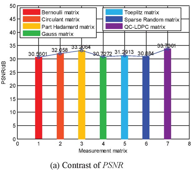
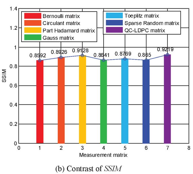
Figure 3 Comparison of parameters by different matrices.

Where $Q$ represents the grayscale level of the quantization, $g(i,j)$ is taken as the original image, and $g^{\prime }(i,j)$ is reconstructed image. $M$ and $N$ represents the length and width of the image respectively.

SSIM (structural similarity index) is an index for the similarity of two images, expressed by the following formula

$$\mathrm{𝑆𝑆𝐼𝑀}(x,y)=\frac{(2{\mu }_x{\mu }_y+c_1)(2{\sigma }_{xy}+c_2)}{({\mu }_x^2+{\mu }_y^2+c_1)({\sigma }_x^2+{\sigma }_y^2+c_2)}$$

(17)

where $x$ and $y$ are the two images with similar structures, ${\mu }_x$ is the mean of $x$, ${\sigma }_x^2$ is the variance of $x$, ${\sigma }_y^2$ is the variance of $y$, and ${\sigma }_{xy}$ is the covariance of $x$ and $y$. $c_1$ and $c_2$are constants used to maintain stability. $c_1={(k_{1}L)}^2$,$c_2={(k_{2}L)}^2$, $L$ represents the dynamic range of pixel values. $k_1=0.01$, $k_2=0.03$.

NMSE (normalized mean square error) is defined as

$$\mathrm{𝑁𝑀𝑆𝐸}=\frac{{\sum }_{i=1}^M{\sum }_{j=1}^N{[g^{\prime }(i,j)-g(i,j)]}^2}{{\sum }_{i=1}^M{\sum }_{j=1}^N{[g(i,j)]}^2}$$

(18)

where $g(i,j)$ is taken as the original image, and $g^{\prime }(i,j)$ is reconstructed image. $M$ and $N$ represents the length and width of the image respectively.

It is shown in Figure 3 the comparison parameters of PSNR, SSIM, NMSE and Runtime in image recovery of Bernoulli matrix, circulant Matrix, Gaussian matrix, part Hadamard matrix, random sparse matrix, Toeplitz matrix and QC-LDPC measurement matrix. According to the data in Figure 3, the image recovered by QC-LDPC measurement matrix has the best effect, with PSNR at 33.7301dB, structural similarity at 0.9219 and NMSE at 0.0024. In second, the part Hadamard matrix PSNR was 33.2064 dB, the structural similarity was 0.9128, and the NMSE was 0.0025. This is mainly because the two kinds of measurement matrices have good orthogonality in structure, and the finite geometry structure QC-LDPC matrix designed in this paper eliminates the short girth and reduces the complexity of coding and decoding by optimizing the design of the basis matrix.

On the other hand, through the comparison of Runtime, it is found that QC-LDPC matrix spends the least time in image recovery, Runtime is 7.9955s. The second is gauss matrix, and the Runtime is 8.2426s. This is mainly because the measurement matrix is a very sparse matrix with low density, and has the structural characteristics of cyclic or quasi-cyclic, which greatly improves the operation speed. However, the Gaussian matrix is irrelevant to the vector elements of most orthogonal sparse basis. The measurement matrix can satisfy the RIP criterion with high probability and recover the K sparse signal with length N from the high probability of M measured values. In addition, the shift register can be used in the hardware implementation of QC-LDPC matrix, which can save the storage space of check matrix and meet the demand of real-time transmission.

4 Conclusion

The compressed sensing theory solves the problem of bandwidth in traditional sampling. The measurement matrix with good performance projects the signal into the low dimensional space, and the measured value contains as much important information of the original signal as possible, so as to ensure the accurate recovery of the original signal. In view of the problems such as large data transmission and difficult hardware implementation in using traditional measurement matrix for data compression, it is constructed QC-LDPC codes by cyclic shift structure of the basis matrix, which can eliminate the short girth of 4 in Tanner graph and improve decoding threshold through the optimization design of basis matrix structure. Because of its characteristics of cycle or quasi cycle, it can not only save the check matrix of storage space but also reduce the decoding complexity, so as to be suitable for application in integrated circuits. It can be realized by simple shift register in coding, so it can save cost in practice. Through the comparison of simulation data of image recovery, it is found that the recovery results of QC-LDPC matrix are better than other traditional measurement matrices by using the same OMP algorithm, and there are good improvements in the aspects of PSNR, SSIM and NMSE. At the same time, through the comparison of running time, it is found that the image recovery with QC-LDPC matrix takes less time, which is conducive to the application of compressed sensing algorithm in real-time data transmission.

Acknowledgements

This work is given the support of Jiangsu laboratory of lake environment remote sensing technologies (No. JSLERS-2018-006).

References

[1] Dimakis A G, Smarandache R, Vontobel P O (2012). LDPC codes for compressed sensing. IEEE Transactions on Information Theory, 58(5), 3093–3114.

[2] Li S, Gao F, Ge G, et al (2012). Deterministic Construction of Compressed Sensing Matrices via Algebraic Curves. IEEE Transactions on Information Theory, 58(8), 5035–5041.

[3] Mo Q, Shen Y (2012). A Remark on the Restricted Isometry Property in Orthogonal Matching Pursuit. IEEE Transactions on Information Theory, 58(6), 3654–3656.

[4] Monajemi H, Jafarpour S, Gavish M, et al (2013). Deterministic Matrices Matching the Compressed Sensing Phase Transitions of Gaussian Random Matrices. Proceedings of the National Academy of Sciences of the United States of America (PNAS), 110(4), 1181–1186.

[5] Li S, Ge G (2014). Deterministic Sensing Matrices Arising From Near Orthogonal Systems. IEEE Transactions on Information Theory, 60(4), 2291–2302.

[6] Amini A, Marvasti F (2011). Deterministic Construction of Binary, Bipolar, and Ternary Compressed Sensing Matrices. IEEE Transactions on Information Theory, 57(4), 2360–2370.

[7] Xin-Ji Liu, Shu-Tao Xia, Fang-Wei Fu (2017). Reconstruction Guarantee Analysis of Basis Pursuit for Binary Measurement Matrices in Compressed Sensing. IEEE Transactions on Information Theory, 63(5), 2922–2932.

[8] Amini A, Montazerhodjat V, Marvasti F (2012). Matrices With Small Coherence Using p-Ary Block Codes. IEEE Transactions on Signal Processing, 60(1), 172–181.

[9] Yu N Y, Zhao N (2013). Deterministic Construction of Real-Valued Ternary Sensing Matrices Using Optical Orthogonal Codes. IEEE Signal Processing Letters, 20(11), 1106–1109.

[10] Mohades M M, Mohades A, Tadaion A (2014). A Reed-Solomon Code Based Measurement Matrix with Small Coherence. IEEE Signal Processing Letters, 21(7), 839–843.

[11] Haiyang Liu, Hao Zhang, Lianrong Ma (2017). On the Spark of Binary LDPC Measurement Matrices From Complete Protographs. IEEE Signal Processing Letters, 24(11), 1616–1620.

[12] Rosnes E, Ambroze M A, Tomlinson M (2014). On the Minimum Stopping Distance of Array Low-Density Parity-Check Codes. IEEE Transactions on Information Theory, 60(9), 5204–5214.

[13] Zhang Yi, Da Xinyu (2015). Construction of girth-eight QC-LDPC codes from arithmetic progression sequence with large column weight. Electronics Letters, 51(16), 1257–1259.

[14] Tasdighi A, Banihashemi A H, Sadeghi M R (2017). Symmetrical constructions for regular girth-8 QC-LDPC codes. IEEE Transactions on Communications, 65(1), 14–22.

[15] Needell D, Vershynin R (2010). Signal recovery from incomplete and inaccurate measurements via regularized orthogonal matching pursuit. IEEE Journal of Selected Topics in Signal Processing, 4(2), 310–316.

Biographies

Xiaoqi Yin is a professor of Huaiyin Institute of Technology. She graduated from Hohai University with a bachelor’s degree in industrial automation in 1997. In 2006, she graduated from Nanjing Normal University, majoring in physics and electronics, and got a master’s degree. Now she is working for the doctorate in China University of Mining and Technology. She is engaged in wireless communication and signal processing.

Jiansheng Qian is a professor, and he is a doctoral supervisor of China mining university. In 1985, he graduated from Northwest Telecommunication Engineering College with a bachelor’s degree in laser. In 1988, he graduated from Xi’an Institute of Optics and Precision Mechanics, Chinese Academy of Sciences with a master’s degree in optoelectronics. He was awarded the title of professor in 2001 and obtained the doctor’s degree in 2003. Now he is the academic leader of the doctoral program of communication and information system in China University of Mining and Technology. His research areas include broadband network technology and application, mine communication and monitoring, optoelectronic technology and application.

Xingge Guo is an associate professor, and he is a master supervisor of China mining university. He received his Bachelor’s degree in electronics and Information Technology in 2001,and received his Master’s degrees in communications and Information Technology in 2006. In 2013, he obtained his doctorate in communication and Information System from China University of Mining and Technology. He is mainly engaged in mine internet of things technology, mine communication and monitoring and mobile communication technology.

Guohua Lin is an associate professor. From 2009 to 2012, he was engaged in the research of electromagnetic wave propagation in the Department of Information Science and Electronic Engineering of Zhejiang University. He received his Ph.D. degree in electromagnetic field and microwave technology from Nanjing University of Posts and Telecommunications in 2015. Since 2018, he has been a teacher in the Faculty of Electronic Information Engineering of Huaiyin Institute of Technology. His research interests include radio wave propagation theory and its applications.

Journal of Web Engineering, Vol. 19_7-8, 999–1016.
doi: 10.13052/jwe1540-9589.19784
© 2020 River Publishers

Abstract

1 Introduction

2 Methodology and Related Works

2.1 Compressed Sensing of Signals

2.2 LDPC Codes

2.3 Construction of QC-LDPC Measurement Matrix

2.3.1 Characteristics of QC-LDPC codes based on finite field

2.3.2 QC-LDPC Matrix Construction Algorithm

3 Simulation Results

4 Conclusion

Acknowledgements

References

Biographies