Research on Indoor Wireless Positioning Precision Optimization Based on UWB

Hua Guo*, Mengqi Li, Xuejing Zhang, Qian Liu and Xiaotian Gao

College of Electronic and Information Engineering, Shandong University of Science and Technology, Qingdao 266590, Shandong, China

E-mail: stone_strong@163.com

*Corresponding Author

Received 25 August 2020; Accepted 10 September 2020; Publication 16 December 2020

Abstract

The ultra-wide band (UWB) indoor positioning precision often has large deviations due to environmental influences. To reduce noise error and improve the UWB indoor positioning precision, this paper divides the indoor positioning into static positioning and mobile positioning, and proposes different optimization algorithms for the two positioning modes. An improved self-organizing feature mapping neural network clustering algorithm is used for static positioning. After training, the layout of the neural network is established, and each weight vector is located at the center of the input vector cluster. Experiments indicate that the fully trained neural network can effectively filter noise, and reduce the mean square error significantly within $3.0\times {10}^{-3}$. The positioning precision is 32.39% and 17.24% higher than those of the K-mean filtering algorithm and the Kalman filtering algorithm. For mobile positioning, the optimized neural network clustering algorithm is integrated with the unscented Kalman filter (UKF) to smooth the positioning data and reduce non-line-of-sight (NLOS) error. Experiments prove that this method can effectively reduce the errors caused by the NLOS state change, and estimate the distance with a high precision for ultra-wide band positioning and tracking.

Keywords: UWB, positioning, neutral network, clustering, Kalman filtering.

1 Introduction

As an ideal choice for indoor low-power consumption and high-speed wireless communication, the ultra-wide band (UWB) wireless technology has been applied in wireless communication and attracted a significant amount of interest. In addition to communication, the UWB system can provide users with high-precision position estimation and tracking capabilities [1–3]. In the UWB communication system, generally non-line-of-sight (NLOS) path blocking between station location and mobile targets will severely reduce the positioning precision. Thus, a proper NLOS error identification and filtering algorithm needs to be designed for improving the positioning precision of the UWB wireless positioning system.

Researchers working on the indoor wireless positioning technology proposed a few effective positioning optimization technologies and algorithms. In Ref. [4], the authors identify and eliminate NLOS errors by using the improved offset Kalman filter. By combining the bias corrected Kalman filter and sliding window, the NLOS errors can be identified and reduced to some extent. This method is mainly used for one way range positioning. In Ref. [5], an integrated indoor positioning system (IPS) combining IMU and UWB through the extended Kalman filter (EKF) and unscented Kalman filter (UKF) was proposed to improve the robustness and accuracy,and the simulation results show that the prior information provided by IMU can significantly suppress the observation error of UWB. In Ref. [6], the authors propose an incremental smoothing method based on the graphic base kernel function to fuse the UWB and pedestrian dead reckoning (PDR) data, and validate the better robustness and higher positioning precision of the incremental smoothing algorithm compared to the robust extended Kalman filter (EKF) algorithm. In Ref. [7], the authors propose an optimization method for positioning precision based on Kalman filtering combined with the inertial navigation system (INS). The authors show that the fusion positioning algorithm is more precise than the single positioning system and can have better positioning performance in a complex indoor environment. In Ref. [8], the authors reduce non-direct firing errors in the indoor environment by using the non-direct firing suppression technology of Kalman filtering. The authors process the time difference data using the extended Kalman filter (EKF) to realize mobile positioning and tracking. Ref. [9] proposed a federated extended finite impulse response (EFIR) filter which includes sub-filters and main filter for INS/UWB human positioning, and proved that the proposed method is better than the traditional federated extended Kalman filter in position accuracy.

This paper proposes a distance estimation system for the UWB technology based indoor positioning system. The proposed system is established on the neutral network clustering algorithm and unscented Kalman filter (UKF) under actual conditions and divides the positioning into static positioning and mobile positioning for optimization. For the static positioning, this paper proposes an improved neutral network clustering algorithm to optimize the positioning algorithm based on time of arrival (TOA). The proposed algorithm filters the noise error within a larger range. For the mobile positioning, this paper proposes a positioning model to improve the positioning precision of mobile targets based on a self-defined UKF algorithm. Experiments show that this method can significantly optimize the UWB indoor positioning. The static positioning and dynamic positioning precisions are within 5 cm and 15 cm, respectively.

2 Optimized Design of Static Positioning Based on Neutral Network Clustering Algorithm

2.1 Principle of UWB Wireless Positioning

The UWB technology is a wireless carrier communication technology, which transmits data by replacing the sine carrier with a narrow non-sine pulse. Thus, it has a very wide spectrum and is applicable to high-speed and short-distance wireless personal communication. The UWB technology can identify a position based on the TOA positioning method. This method can fully detect the signal delay by using the high ultra-broadband signal time resolution at the receiver to estimate the distance from the target node to the reference base station. The positioning algorithm based on the TOA is divided into two stages. The first stage is the ranging stage, in which the distance between the nodes is calculated based on the TOA. The second stage is the positioning stage, in which the positions of the unknown nodes are calculated using specific positioning algorithms based on the distance information obtained from the first stage [10–12].

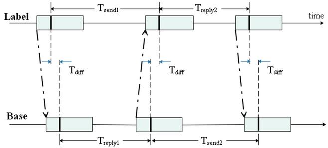
Figure 1 DS-TWR principle.

The ranging algorithm used by the UWB technology is the double-side two-way ranging (DS-TWR) algorithm, which is an extension of the basic single-side two-way ranging. In this type of ranging, two round trip time measurements are combined to get the fly time results. The advantage of this method is that the measurement error will be reduced even in a long response delay [13–16]. The concept of the DS-TWR is shown in Figure 1. First, the Label node sends a signal, and the Base node responds after receiving the signal. Then, the Base node transmits a signal, and the Label node responds after receiving the signal. All base stations and labels will accurately mark the transmission and receiving time of signals in this period, and the single-trip time for transferring pulse signals between nodes is obtained via (1) as follows:

$${\mathrm{T}}_{diff}=\frac{(T_{send1}\times T_{send2}-T_{reply1}\times T_{reply2})}{(T_{send1}+T_{send2}+T_{reply1}+T_{reply2})}$$

(1)

The obtained single-trip time for signal transfer is multiplied by the pulse signal transfer speed, which is almost equal to the speed of light, to obtain the distance between the nodes.

The positions of the mobile stations can be obtained by using the distance measured from the signal sources to base stations, with the base station node as the center and the distance as the radius. As shown in Figure 2, the TOA can be used to identify the position of the target points by using the trilateration algorithm. The base stations are represented by B${}_1$, B${}_2$ and B${}_3$, and M is the mobile station. Assuming that the coordinates of the base station positions are B${}_1$(x${}_1$,y${}_1$), B2(x${}_2$,y${}_2$) and B${}_3$(x${}_3$,y${}_3$), the coordinates of the mobile station are (x, y), and d${}_1$, d${}_2$ and d${}_3$ are distances between the base stations and mobile stations, respectively. The coordinates of the mobile station nodes can be obtained by solving the following equation set:

$$\{\begin{array}{c}\hfill {(x-x_1)}^2+{(y-y_1)}^2={(d_1)}^2\hfill \\ \hfill {(x-x_2)}^2+{(y-y_2)}^2={(d_2)}^2\hfill \\ \hfill {(x-x_3)}^2+{(y-y_3)}^2={(d_3)}^2\hfill \end{array}$$

(2)

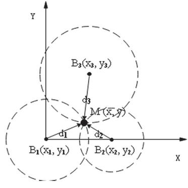
Figure 2 TOA positioning method.

Equation (2) can be arranged as follows:

$$\{\begin{array}{c}\hfill 2x\left(x_1-x_2\right)+2y\left(y_1-y_2\right)=r_1\hfill \\ \hfill 2x\left(x_1-x_3\right)+2y\left(y_1-y_3\right)=r_2\hfill \\ \hfill 2x\left(x_2-x_3\right)+2y\left(y_2-y_3\right)=r_3\hfill \end{array}$$

(3)

where

$$\{\begin{array}{c}\hfill r_1=x_2{}^2-x_3{}^2+y_2{}^2-y_3{}^2+d_3{}^2-d_2{}^2\hfill \\ \hfill r_2=x_1{}^2-x_2{}^2+y_1{}^2-y_2{}^2+d_2{}^2-d_1{}^2\hfill \\ \hfill r_3=x_1{}^2-x_3{}^2+y_1{}^2-y_3{}^2+d_3{}^2-d_1{}^2\hfill \end{array}$$

(4)

Equation (3) can be expressed in a linear form of AX = b, where

$$A=\left[\begin{array}{cc}\hfill 2\left(x_1-x_2\right)\mathit{\hspace{1em}}\hfill & \hfill 2\left(y_1-y_2\right)\hfill \\ \hfill 2\left(x_1-x_3\right)\mathit{\hspace{1em}}\hfill & \hfill 2\left(y_1-y_3\right)\hfill \\ \hfill 2\left(x_2-x_3\right)\mathit{\hspace{1em}}\hfill & \hfill 2\left(y_2-y_3\right)\hfill \end{array}\right]\mathit{\hspace{1em}}X=\left[\begin{array}{c}\hfill x\hfill \\ \hfill y\hfill \end{array}\right]\mathit{\hspace{1em}}b=\left[\begin{array}{c}\hfill r_1\hfill \\ \hfill r_2\hfill \\ \hfill r_3\hfill \end{array}\right]$$

Equation (3) includes three equations and two unknown parameters, and belongs to a statically indeterminate equation set, which should be solved using the non-linear least square method. The error function is established according to the parameters and geometric positions of the three base stations. The Taylor series expansion method is used to approximate the calculations for minimizing the error function and identifying the coordinate position of the mobile stations.

2.2 Design of Self-Organizing Map (SOM)

For the UWB positioning technology, the indoor positioning data will approximately have about 80 cm of positioning error in practice due to the influence of hardware and indoor environment. These data can be represented as the Gaussian distribution around the true values, as shown in Figure 3. In the past, the research work focused on optimization of the ranging algorithm. However this research work consisted of complicated processing and included a few algorithms that were not suitable for distance measurement such as the two-way ranging. The neutral network clustering algorithm is better suited for handling such cases. It is an unsupervised learning algorithm that has a simple structure and higher processing speed, can effectively reduce the error magnitude, and is highly suitable for research on positioning precision optimization [17–21]. For UWB positioning, the positioning values are clustered via the optimized SOM neutral network and the optimization capabilities of the neutral network clustering algorithm for wireless indoor positioning are tested and analyzed.

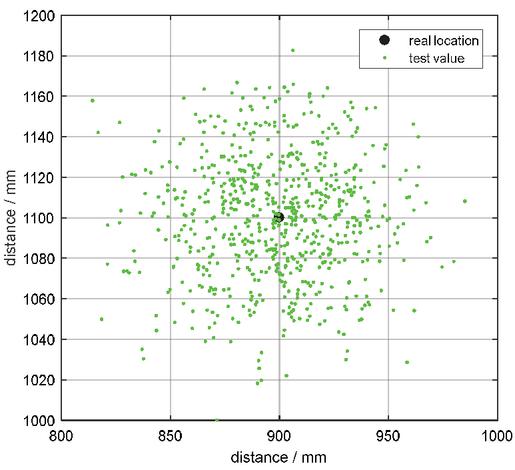
Figure 3 UWB positioning test value and true coordinate points.

2.2.1 Self-Organizing Neutral Network

The SOM neutral network is based on the traditional competitive network. It emulates the biologically active areas, suppresses surrounding feedback coupling, which has high generalization ability. The traditional competitive network only includes two layers and its structure is shown in Figure 4. The output layer is also called the core layer. Only one output neutral cell is selected during a single calculation, and the selected neutral cell is marked as 1 and the other neutral cells are marked as 0. The excitation of the selected neutral cell will be further strengthened by weight modulation and the excitation of the other neutral cells will be unchanged. The competitive neutral network obtains sample distribution information in a competitive leaning manner.

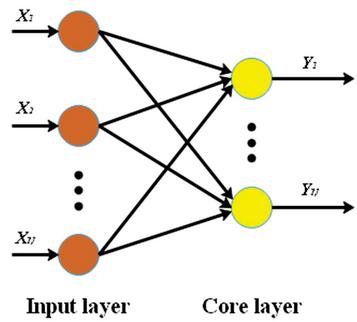
Figure 4 Structure of competitive neutral network.

The characteristic of SOM is that the nodes of the core layer are topologically related. The input and output neutral cells are connected with one another via weights. Meanwhile, the adjacent output neutral cells are connected via the weight vectors. We shall determine such topology relation. If we expect a one-dimensional model, the output nodes are connected into a continuous line. If we expect a two-dimensional topology, the output nodes form a plane. As shown in Figure 5, the SOM can discretize the input cells in any dimension into a one-dimensional or two-dimensional discrete space.

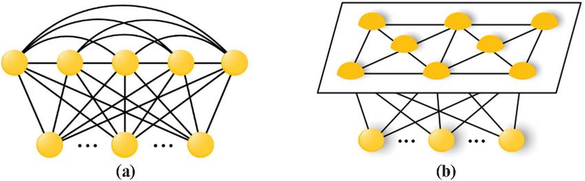
Figure 5 Self-organizing mapping network topology ((a) one-dimensional linear array; (b) two-dimensional linear array).

The relation between a neutral cell vector and an input vector is expressed as the inner product of the two vectors. The sample vectors and weights are normalized. Thus, the calculation of the largest inner product is equivalent to finding the smallest Euclidean distance. As multiple neutral cell vectors exist, multiple distance values can be obtained. All the obtained inner product values are compared, and the maximum value is retained. This process indicates competition between the neutral cells. As shown in Figure 6, the inner product between the neutral cell vector $W_2$ and input vector $P_1$ is larger and the inner product between the neutral cell vector $W_1$ and input vector $P_1$ is smaller. Thus, the largest inner product is equivalent to the smallest Euclidean distance.

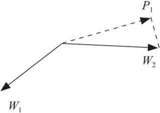
Figure 6 Distance between the neutral cell and input vector.

The selected neutral cells are moved to the input vector according to Kohonen rules shown in (5) and used to update the weights, as shown as Figure 7. The value of the ith input neutral cell is given by $x_i$, $W_{ij}$ is the weight of a neighboring neutral cell connected to $x_i$, and $\eta$ is the learning rate.

$$W_{ij}(q)=W_{ij}(q-1)+\eta (x_i(q-1)-W_{ij}(q-1))$$

(5)

Figure 7 Kohonen rules.

The training units will participate in competition with each other during training and the processing unit with the maximum output is selected as the winner. The winner node can suppress other competitors and active adjacent nodes. Only the winning node generates the output and only the weights between the winner and its adjacent nodes can be adjusted. Several input vectors will affect different neutral cell vectors. After multiple training iterations, all the neutral cell vectors in the network will reach stability. In this case, the competitive network training is completed. The corresponding weight of this neutral cell will simultaneously adjust to the input vectors’ directions and finally become stable at the mean value of the input vectors. In this case, the neutral cell vector points in the direction of the input vector cluster, as shown as Figure 8.

Figure 8 Final weight selection ($P_i$: input sample; $W_i$: neutral cell vector).

The learning rate and neighbor adjustment rules are implemented via the following codes:

if (ls.step$<$lp.order_steps)

percent=1$-$ls.step/lp.order_steps;nd=1.00001+(ls.nd_max-1)$\ast$percent;

lr=lp.tune_lr+(lp.order_lr$-$lp.tune_lr)$\ast$percent;

else

nd=lp.tune_nd+0.00001;

lr=lp.tune_lr$\ast$lp.order_steps/ls.step;

2.2.2 Optimized SOM Algorithm

The number of neutral cells in the output layer is related to the number of samples in the training set: excessive or insufficient neutral cell nodes will affect the algorithm’s performance. Excessive neutral cells may result in dead neutral cells. Thus, it is particularly important to determine the topology and training steps in the self-organizing network clustering algorithm, and it is necessary to determine the most suitable mapping topology by different combinations and the corresponding experiments. The ranking mode of the nodes at the output layer depends on the actual application requirement and should intuitively reflect the physical meaning of actual problems as much as possible.

By combining the high transmission rate of the UWB technology, a group of data is collected every 500 ms, and each group includes 200 nodes for analysis. Based on experiments, we discovered that the optimal topology in the positioning environment is a $3\times 2$ two-dimensional structure with six neutral cells at the output layer, as shown in Figure 9. When the number of the training steps is about 500, the classification results are the most detailed. In this case, the mean square error remains stable at about $2\times {10}^{-3}$, and the classification results satisfy the precision requirement. Partial test data are shown in Tables 1 and 2.

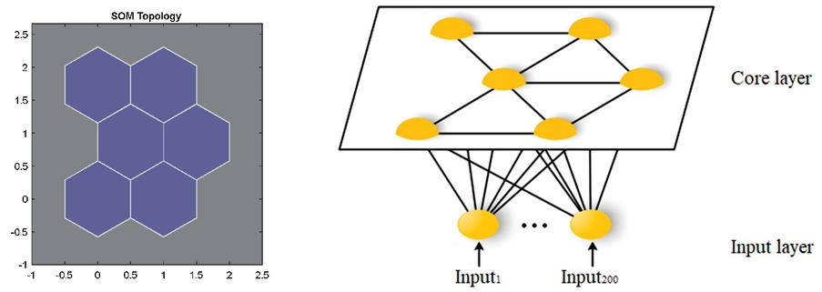
Figure 9 Schematic diagram of $3\times 2$ dimensional topology obtained based on experiments and SOM network structure.

Table 1 Positioning mean square error for partial topology

Anchor	Mean square error of each topology
point	[1, 1]	[1, 2]	[2, 1]	[2, 2]	[3, 1]	[3, 2]	[4, 1]	[4, 2]	[4, 3]	[5, 1]	[5, 2]	[5, 3]
(7, 11)	0.0435	0.0109	0.0049	0.0270	0.0144	0.0016	0.0085	0.0112	0.0080	0.0099	0.0036	0.0061
(8, 5)	0.0412	0.0114	0.0042	0.0185	0.0119	0.0019	0.0077	0.0123	0.0110	0.0105	0.0050	0.0052

Table 2 Clustering results of network with different training times

Epoch	Clustering results						MSE
10	3	121	132	145	2	97	0.1363
30	2	5	161	166	2	164	0.1099
50	5	7	172	152	0	164	0.0854
100	105	71	50	107	100	67	0.0549
200	80	78	132	77	65	68	0.0015
500	84	80	122	74	62	78	0.0018
1000	97	74	149	57	66	57	0.0062

Figure 10 shows the distribution of cumulative errors for different topologies. From this figure, the values of the clustering-optimized positioning points for the $3\times 2$ topology are better than the values of other topologies. Clustering optimization under this topology can significantly reduce the positioning errors.

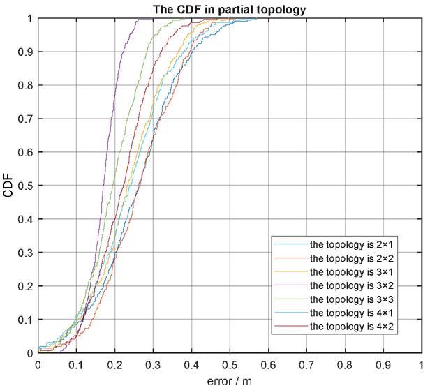
Figure 10 Distribution of cumulative errors for partial topology.

The center points of different classes under the $3\times 2$ dimensional topology are shown in the following figure. When the coordinates of the positioning point are (7.00, 11.00), the class containing the coordinate point with the center value of (6.9428,10.9639) has far more test points than other classes, and the center point value is more approximate to true value, as shown in Figure 11.

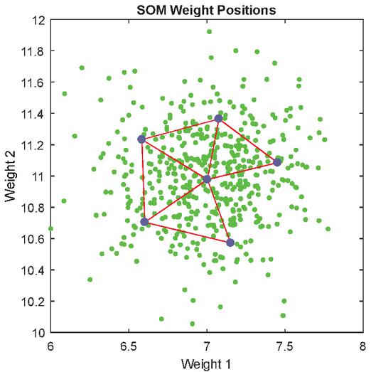
Figure 11 Positioning experiment result of the $3\times 2$ dimensional SOM network.

When the input vector clusters are close to one another at the network competition layer, it is highly possible that one neutral cell vector representing a cluster intrudes into the area represented by another neutral cell vector, which will destruct current classification. Alternatively, when the initial neutral cell vector is too far from the input vectors, this neutral cell vector cannot learn all the time and becomes a dead neutral cell. In this case, the Euclidean distance between the clustering models obtained from the positioning points is used as a parameter to measure the distance between the neutral cell vectors, and the calculated results are retrained. When the Euclidean distance of these clusters reaches the set threshold, the iterative training is terminated.

3 Optimized Design of Dynamic Positioning of Neutral Network Clustering Algorithm Combined with Unscented Kalman Filter

This section introduces the UKF algorithm in dynamic positioning to model the positioning environment and establish a kinematic model for the mobile stations. The Kalman filtering algorithm is integrated with the optimal neutral network algorithm structure obtained for static positioning in the previous section to filter the environmental errors as much as possible and further optimize the dynamic positioning precision. The UKF combines the unscented transform (UT) with standard Kalman filter system, which is a non-linear filtering method proposed by Julier et al. [22]. This algorithm is mainly based on the idea of Kalman filtering and uses sampling points to calculate the predicted and measured values of the targets at subsequent time-instants. Such a filter can effectively overcome the defects of Kalman filtering such as low estimation precision and stability, and has a higher precision in the processing of non-linear problems [23–26].

3.1 Principle of Unscented Transform

Assume a non-linear transform $y=f(x)$, in which the state vector x is an n-dimensional random variant, with a mean value of $\overline{x}$ and variance of P. The $(2n+1)$ Sigma points $X$ and the corresponding weights $\omega$ can be obtained via the following UT to calculate the statistical features of $y$.

• Calculate the $(2n+1)$ Sigma points (sampling points), where $n$ indicates the dimension of the state.

$$\{\begin{array}{cc}{X}^{(0)}=\overline{X},\hfill & i=0\hfill \\ X^{(i)}=\overline{X}+{(\sqrt{(n+\lambda )P})}_i,\hfill & i=1\sim n\hfill \\ X^{(i)}=\overline{X}-{(\sqrt{(n+\lambda )P})}_i,\hfill & i=n+1\sim 2n\hfill \end{array}$$

(6)

In this equation, ${(\sqrt{P})}^T(\sqrt{P})=P$ and ${(\sqrt{P})}_i$ indicate the ith row of the matrix root.

• Calculate the corresponding weights of the sampling points.

$$\{\begin{array}{c}{\omega }_m^{(0)}=\frac{\lambda }{n+\lambda }\hfill \\ {\omega }_m^{(0)}=\frac{\lambda }{n+\lambda }+(1-{\alpha }^2+\beta )\hfill \\ {\omega }_m^{(i)}={\omega }_c^{(i)}=\frac{\lambda }{n+\lambda },i=1\sim 2n\hfill \end{array}$$

(7)

In this equation, the subscripts m and c refer to the mean value and covariance, respectively. The superscript is the ith sampling point. The parameter $\lambda ={\alpha }^2(n+\kappa )-n$ is a scaling parameter used to reduce the total prediction error. The coefficient $\alpha$ is selected to control the distribution state of the sampling points and $\kappa$ is an optional parameter, which is used to ensure that the matrix $(n+\lambda )P$ is a positive semidefinite matrix. A non-negative weight coefficient $\beta$ can consolidate the high-order moment in the equation so that the influence of high-order items can be included.

3.2 Implementation of Unscented Kalman Filter Algorithm

For a time instant $k$, the non-linear system composed of the random variable $X$ with Gaussian white noise $W(k)$, and the observation variable Z with Gaussian white noise $V(k)$ is described by (8).

$$\{\begin{array}{c}X(k+1)=f(X(k),W(k))\hfill \\ Z(k)=h(X(k),V(k))\hfill \end{array}$$

(8)

Assume that the covariance matrices of $W(k)$ and $V(k)$ are represented by $Q$ and $R$, respectively. The basic steps of the unscented filtering algorithm of the random variable $X$ at a time instant $k$ are described as follows:

A group of sampling points (sigma point set) and their corresponding weights can be obtained using (5) and (6).

$$X^{(i)}(k|k)={\left[\begin{array}{c}\widehat{X}(k|k)\hfill \\ \widehat{X}(k|k)+\sqrt{(n+\lambda )P(k|k)}\hfill \\ \widehat{X}(k|k)-\sqrt{(n+\lambda )P(k|k)}\hfill \end{array}\right]}^T$$

(9)

Calculate one-step prediction of the Sigma point set, $i=1,2,\mathrm{\dots }2n+1$ as follows:

$$X^{(i)}(k+1|k)=f[k,X^{(i)}(k|k)]$$

(10)

Calculate one-step prediction and covariance matrix of the system state variant as follows:

$\widehat{X}(k+1|k)$	$={\displaystyle \sum _{i=0}^{2n}}{\omega }^{(i)}{X}^{(i)}(k+1|k)$	(11)
$P(k+1|k)$	$={\displaystyle \sum _{i=0}^{2n}}{\omega }^{(i)}[\widehat{X}(k+1|k)-X^{(i)}(k+1|k)]$
	$\mathrm{\hspace{1em}}\times {[\widehat{X}(k+1|k)-X^{(i)}(k+1|k)]}^T+Q$	(12)

Generate new Sigma point sets by using UT according to the one-step prediction values as follows:

$$X^{(i)}(k+1|k)={\left[\begin{array}{c}\hfill \widehat{X}(k+1|k)\hfill \\ \hfill \widehat{X}(k+1|k)+\sqrt{\left(n+\lambda \right)P(k+1|k)}\hfill \\ \hfill \widehat{X}(k+1|k)-\sqrt{(n+\lambda )P(k+1|k)}]\hfill \end{array}\right]}^T$$

(13)

After the updated Sigma point sets are substituted into the observation equation, the predicted observation can be obtained as

$$Z^{(i)}(k+1|k)=h[X^{(i)}(k+1|k)]$$

(14)

The mean and covariance of the system prediction are obtained by the following weighted sum:

$\overline{Z}(k+1|k)$	$={\displaystyle \sum _{i=0}^{2n}}{\omega }^{(i)}{Z}^{(i)}(k+1|k)$	(15)
$P_{Z_k{Z}_k}$	$={\displaystyle \sum _{i=0}^{2n}}{\omega }^{(i)}[Z^{(i)}(k+1|k)-\overline{Z}(k+1|k)]$
	$\mathrm{\hspace{1em}}\times {[Z^{(i)}(k+1|k)-\overline{Z}(k+1|k)]}^T+R$	(16)
$P_{X_k{Z}_k}$	$={\displaystyle \sum _{i=0}^{2n}}{\omega }^{(i)}[X^{(i)}(k+1|k)-\widehat{X}(k+1|k)]$
	$\mathrm{\hspace{1em}}\times {[Z^{(i)}(k+1|k)-\overline{Z}(k+1|k)]}^T$	(17)

Calculate the Kalman gain matrix as

$$\mathrm{K}(k+1)=P_{X_k{Z}_k}P^{-1}{}_{Z_k{Z}_k}$$

(18)

Update the system state and covariance as follows:

$\widehat{X}(k+1|k+1)=\widehat{X}(k+1|k)+K(k+1)[Z(k+1)-\widehat{Z}(k+1|k)]$	(19)
$P(k+1|k+1)=P(k+1|k)-K(k+1)P_{Z_k{Z}_k}{K}^T(k+1)$	(20)

3.3 Model Design of Unscented Kalman Filtering in Dynamic Positioning

Consider a mass point $M$ moving on a two-dimensional plane $x-y$. It undergoes approximately uniformly accelerated linear motion in the horizontal direction ($x$-axis direction) and similar uniformly accelerated motion in the vertical direction ($y$-axis direction). Assuming the sampling time as $T$, and $s(k)$ and $y(k)$ indicate the true position of the mobile station and the positioning observation value at kT, respectively. The following observation model can be obtained:

$$z(k)=s(k)+v(k)$$

(21)

In this equation, $v(k)$ indicates the positioning error, i.e., the observation noise. Assume that $v(k)\sim N(0,{\sigma }_v^2)$, where ${\sigma }_v^2$ is obtained from a large number of positioning observation test data using the statistical method. Set the rate of the mobile station at time kT as $\dot{s}(k)$ and the acceleration as $\ddot{s}(k)$. Using the uniform acceleration motion equation, we can get:

$s(k+1)$	$=s(k)+\dot{s}(k)T+0.5\ddot{s}(k)T^2$
$\dot{s}(k+1)$	$=\dot{s}(k)+\ddot{s}(k)T$	(22)

The system state $x(k)$ at the sampling time kT is given by the position, rate and acceleration, namely:

$$x(k)=\left[\begin{array}{c}\hfill s(k)\hfill \\ \hfill \dot{s}(k)\hfill \\ \hfill \ddot{s}(k)\hfill \end{array}\right]$$

(23)

We can get the state equation of the mobile station undergoing motion as follows:

$$\left[\begin{array}{c}\hfill s(k+1)\hfill \\ \hfill \dot{s}(k+1)\hfill \\ \hfill \ddot{s}(k+1)\hfill \end{array}\right]=\left[\begin{array}{ccc}\hfill 1\mathit{\hspace{1em}}\hfill & \hfill T\mathit{\hspace{1em}}\hfill & \hfill 0.5T^2\hfill \\ \hfill 0\mathit{\hspace{1em}}\hfill & \hfill 1\mathit{\hspace{1em}}\hfill & \hfill T\hfill \\ \hfill 0\mathit{\hspace{1em}}\hfill & \hfill 0\mathit{\hspace{1em}}\hfill & \hfill 1\hfill \end{array}\right]\left[\begin{array}{c}\hfill s(k)\hfill \\ \hfill \dot{s}\left(k\right)\hfill \\ \hfill \ddot{s}(k)\hfill \end{array}\right]+\omega (k)$$

(24)

The observation equation is given as follows:

$$z(k)=[1\mathit{\hspace{1em}}0\mathit{\hspace{1em}}0]\left[\begin{array}{c}\hfill s(k)\hfill \\ \hfill \dot{s}(k)\hfill \\ \hfill \ddot{s}(k)\hfill \end{array}\right]+v(k)$$

(25)

The state space model of the system is as follows:

$𝒙(k+1)$	$=𝚽𝒙(k)+\omega (k)$
$𝒛(k)$	$=𝑯𝒙(k)+v(k)$	(26)

Now the above model is extended to the two dimensional coordinate system and the position, rate and acceleration are expressed using the vector $𝑿(k)={[x_k,y_k,{\dot{x}}_k,{\dot{y}}_k,{\ddot{x}}_k,{\ddot{y}}_k]}^T$ at time $k$. Considering the additive system noise $W(k)$ included in the two-dimensional motion, the motion state equation of this mass point under the Descartes coordinate system can be described as follows:

$$𝑿(k+1)=𝚽𝑿(k)+𝑾(k)$$

(27)

where

$$\mathrm{\Phi }=\left[\begin{array}{cccccc}\hfill 1\mathit{\hspace{1em}}\hfill & \hfill 0\mathit{\hspace{1em}}\hfill & \hfill T\mathit{\hspace{1em}}\hfill & \hfill 0\mathit{\hspace{1em}}\hfill & \hfill \frac{T^2}{2}\mathit{\hspace{1em}}\hfill & \hfill 0\hfill \\ \hfill 0\mathit{\hspace{1em}}\hfill & \hfill 1\mathit{\hspace{1em}}\hfill & \hfill 0\mathit{\hspace{1em}}\hfill & \hfill T\mathit{\hspace{1em}}\hfill & \hfill 0\mathit{\hspace{1em}}\hfill & \hfill \frac{T^2}{2}\hfill \\ \hfill 0\mathit{\hspace{1em}}\hfill & \hfill 0\mathit{\hspace{1em}}\hfill & \hfill 1\mathit{\hspace{1em}}\hfill & \hfill 0\mathit{\hspace{1em}}\hfill & \hfill T\mathit{\hspace{1em}}\hfill & \hfill 0\hfill \\ \hfill 0\mathit{\hspace{1em}}\hfill & \hfill 0\mathit{\hspace{1em}}\hfill & \hfill 0\mathit{\hspace{1em}}\hfill & \hfill 1\mathit{\hspace{1em}}\hfill & \hfill 0\mathit{\hspace{1em}}\hfill & \hfill T\hfill \\ \hfill 0\mathit{\hspace{1em}}\hfill & \hfill 0\mathit{\hspace{1em}}\hfill & \hfill 0\mathit{\hspace{1em}}\hfill & \hfill 0\mathit{\hspace{1em}}\hfill & \hfill 1\mathit{\hspace{1em}}\hfill & \hfill 0\hfill \\ \hfill 0\mathit{\hspace{1em}}\hfill & \hfill 0\mathit{\hspace{1em}}\hfill & \hfill 0\mathit{\hspace{1em}}\hfill & \hfill 0\mathit{\hspace{1em}}\hfill & \hfill 0\mathit{\hspace{1em}}\hfill & \hfill 1\hfill \end{array}\right]$$

The positioning base station monitors the targets. The coordinates of the base station are $(x_i,y_i)$, and the position of the mobile station at time $k$ is $x(k),y(k)$). Now the distance between the positioning base station and the mobile station is defined as the observation $Z$. Subsequently, the observation equation can be represented using the following equation:

${𝒁}_{𝒊}(k)=𝒉(𝑿(k))+𝑽(k)=\sqrt{{(x(k)-x_i)}^2+{(y(k)-y_i)}^2}+𝑽(k)$(28)

where $Z_i(k)$ is the distance between the base station and the label obtained by DS-TWR algorithm.

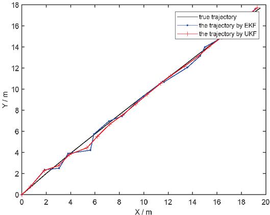
Figure 12 Trajectory of mobile station under different conditions.

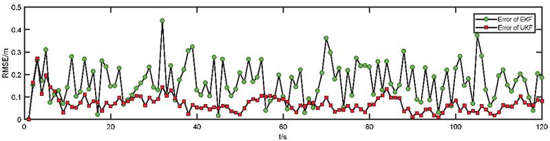
Figure 13 RMSE comparison for two algorithms.

It can be seen from Figure 12 that the positioning trajectory of the UKF algorithm is more precise than that of the extended Kalman filtering (EKF) algorithm in the NLOS environment. To test the positioning performance, the root mean square error (RMSE) is used for comparison [27, 28]. Figure 13 compares the RMSE of the indoor dynamic position based on the optimization of two algorithms. The positioning error of the UKF algorithm is not more than 0.3 m and the positioning error of the EKF algorithm is about 0.5 m in the same environment. This indicates that the UKF algorithm has a higher precision than the EKF algorithm. However, as the number of iterations increases, the positioning error will also increase. Thus, the number of iterations must be carefully selected.

4 Experimental Results and Analysis

Figure 14 shows the experimental site where the experimental plane is horizontal. The positioning node is always fixed at the mobile station in the experiment. To simplify the calculations, it is assumed that the z-axis coordinate of the positioning node is 0, i.e., the horizontal plane where the positioning node is located is used as the xoy plane to establish a three-dimensional rectangular coordinate system. Consequently, only the x and y coordinates of the positioning node are analyzed in the experiment. In the dynamic positioning test, we install the UWB positioning label and laser ranging modules on the mobile station. Two laser ranging modules are used to identify the real-time coordinates of the mobile station in real-time. The installation of the laser ranging module is shown in Figure 15. The two laser ranging modules should always be perpendicular to the wall.

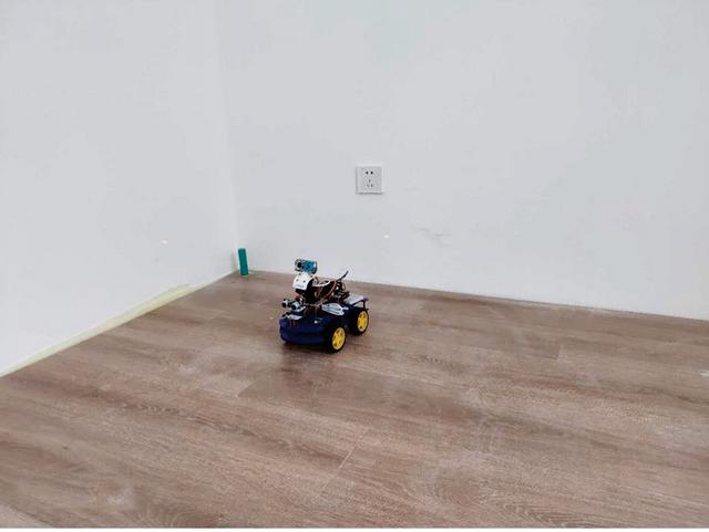
Figure 14 Experimental site.

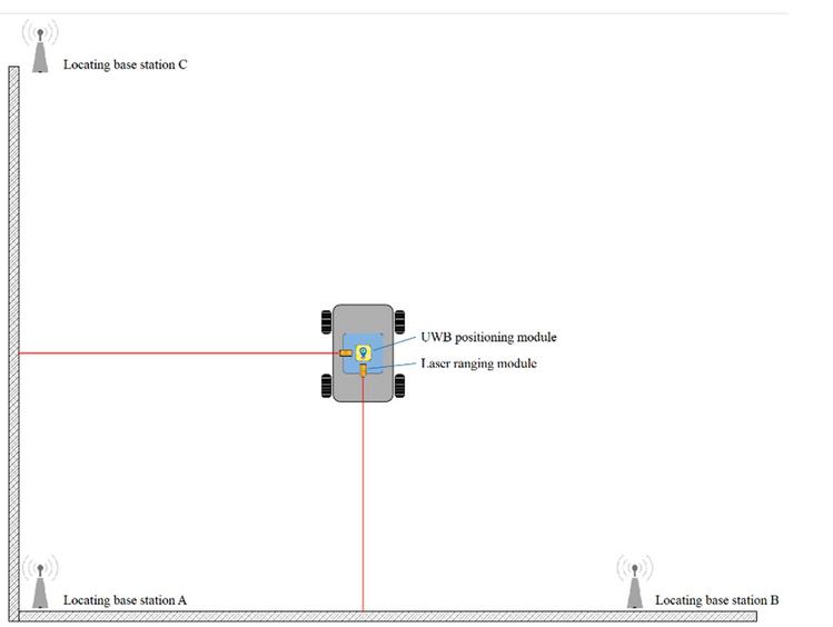
Figure 15 Experiment simulation diagram.

The DW1000 chip produced by DecaWave is selected as the positioning module in the experiment. The positioning module includes three base stations and one positioning label module, and has an effective transmission distance of 300 m. This module supports data rates of 110 Kbps, 850 Kbps and 6.8 Mbps, the positioning module is shown in Figure 16.

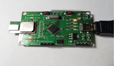
Figure 16 UWB module used in this paper.

To ensure precision of the positioning parameters, the high-precision laser ranging module produced by MyAntenna is used to measure the coordinates of the mobile station. A photo of the module is shown in Figure 17. This module has millimeter-level precision and resolution, and its repetition precision and effective range are $\pm 1$ mm and between 0.1–40 m, respectively. It is highly adaptive to temperature, light or weak signal reflection, and its small size enable it to be easily embedded into the mobile station.

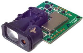
Figure 17 Laser ranging module.

The monitoring software running on PC is programmed with C#. The data are sent and received via the main base station A connected with the PC to complete the positioning of the label. The relative position coordinates of the label and the distance from each base station can be displayed in real time. Figure 18 shows the interface that displays the ranging circle of each base station under the trilateration algorithm in static positioning. The default baud rate of the device is 115,200 bps and the default MODBUS-ID is 1. When only one label is provided, the continuous automatic output mode is started. When multiple labels are provided, the scanning and positioning mode is started, and the positioning information is updated periodically.

Figure 18 Upper PC interface.

4.1 Experimental Data Analysis of Static Positioning

To measure the positioning precision of the UWB indoor wireless network positioning system in the static environment, and the algorithm optimization performance of the neural network, we select several fixed points in the experimental site to place the positioning labels. The positions of the points are shown in Figure 19. Each algorithm is tested separately, and the measured data are analyzed and compared with the actual data.

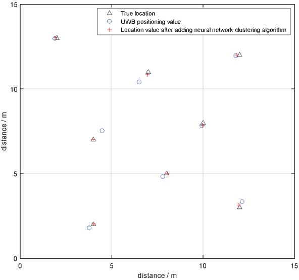
Figure 19 Static positioning.

First, the static points are sampled. A total of 500 sets of original positioning data are selected for each positioning point and optimized using K-mean filtering, Kalman filtering algorithm and neutral network clustering algorithm, respectively. The error in the results obtained using each method is calculated. The calculated error values are shown in Table 3.

Table 3 Positioning values and mean square error for three algorithms

	K-means Clustering Algorithm		Kalman Filtering Algorithm		Neural Network Clustering Algorithm
Anchor Coordinates	Locator Data	MSE	Locator Data	MSE	Locator Data	MSE
(7.00, 11.00)	(7.085, 11.093)	0.0079	(6.972, 11.049)	0.002	(6.972, 11.049)	0.0016
(8.00, 5.00)	(8.076, 5.089)	0.0068	(8.057, 5.041)	0.0025	(8.042, 5.023)	0.0011
(10.00, 8.00)	(10.071, 7.936)	0.0046	(10.051, 7.931)	0.0037	(10.034, 7.961)	0.0013
(12.00, 12.00)	(11.914, 11.912)	0.0076	(11.984, 11.926)	0.0029	(11.956, 11.937)	0.0030
(14.00, 10.00)	(14.081, 10.102)	0.0085	(14.062, 10.055)	0.0034	(14.042, 10.031)	0.0014
(15.00, 9.00)	(14.911, 9.107)	0.0097	(14.927, 9.063)	0.0046	(14.948, 9.044)	0.0023
(17.00, 15.00)	(16.923, 15.084)	0.0065	(17.064, 15.053)	0.0035	(17.043, 15.035)	0.0015
(20.00, 30.00)	(19.924, 30.087)	0.0067	(20.061, 29.966)	0.0024	(20.022, 29.937)	0.0022

It can be seen that using the K-mean filtering, the mean square error (MSE) of the positioning value can reach a maximum value of $9.7\times {10}^{-3}$, and it is below $4.6\times {10}^{-3}$ with the Kalman filtering algorithm. Compared with the positioning test values obtained using these two algorithms, the neutral network clustering algorithm can optimize the precision better, the precision of the test points is also higher, and the MSE remains stable below $3.0\times {10}^{-3}$. Its precision is 44.39% and 19.24% higher than those of the K-mean filtering and Kalman filtering algorithms, respectively. Thus, its optimization effect is significant. Taking the coordinate point (20.00, 30.00) as an example, Figure 20 displays the performance in terms of the test values and error ranges of the three optimization algorithms.

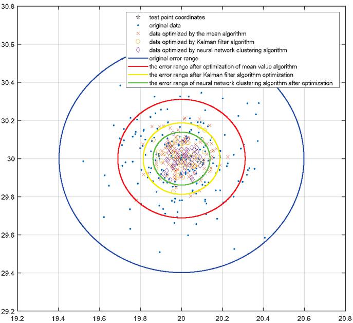
Figure 20 Performance optimization comparison of three algorithms in UWB positioning.

The experimental results show that the clustering algorithm in the static positioning not only significantly improves the positioning precision, but also effectively reduces the position jitter of real-time positioning. Thus, it has an excellent auxiliary effect on improving the positioning precision.

4.2 Experimental Data Analysis of Dynamic Point Positioning

The dynamic point positioning uses the Raspberry Pi smart car as the carrier for the positioning label. The car moves along the predetermined route in the experimental site, and measures and records the data. The moving track of the mobile station is shown in Figure 21. The positioning track results show that although the UWB has better positioning precision, factors such as multi-path effect still influence the positioning precision. The optimized neutral network clustering algorithm used in this paper integrates the UKF algorithm to correct and identify the moving track, which is more precise than single positioning, and can achieve better positioning performance in the complicated indoor environment.

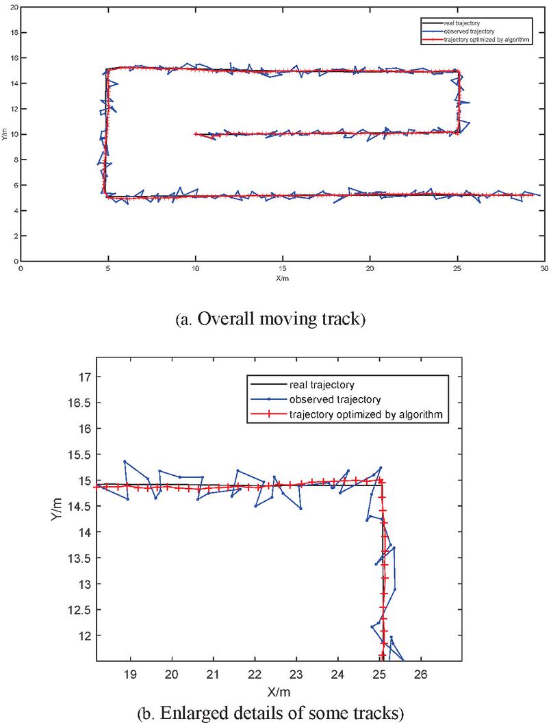
Figure 21 Moving track of mobile station.

We compare the errors before and after optimization in Figure 22. The positioning data become more precise after the fusion algorithm is used for dynamic positioning. The measurement and the subsequent error calculation show that the UWB indoor positioning precision can be reduced to within 15 cm, which clearly demonstrates the optimization performance.

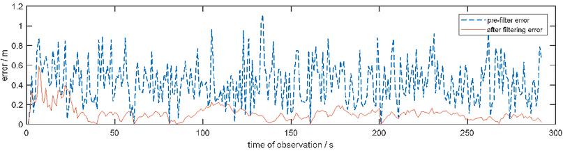
Figure 22 Error comparison before and after optimization.

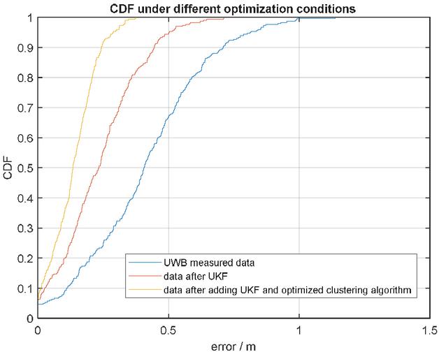
Figure 23 Cumulative distribution of positioning error.

Next, the errors are analyzed and compared. Figure 23 displays the cumulative distribution function (CDF) of the positioning error using different methods. The horizontal and vertical coordinates indicate the positioning error and the cumulative distribution function, respectively. It is clear from the figure that the positioning error is smaller, and the measurement precision is higher after the fusion and optimization using the two algorithms. Without any algorithm optimization, the UWB positioning error in the indoor environment is about 80 cm. When only the UKF algorithm is used for optimization, the error is about 30 cm due to filtering divergence caused by non-local sampling. The yellow line in the figure indicates the results obtained from the fusion system proposed in this paper. It shows that the optimization algorithm that combines the neutral network clustering algorithm and UKF algorithm can improve the precision compared to the individual algorithms. The error in dynamic measurement remains stable within 15 cm. As there are a few limitations to UWB positioning under the UKF optimization, the fusion algorithm that combines the neural network clustering algorithm can significantly improve the positioning precision.

5 Conclusions

To improve the wireless positioning precision in complicated indoor environments, this paper proposed the positioning optimization algorithm based on the fusion of self-organizing mapping (SOM) neural network and unscented Kalman filtering algorithm. This fusion was motivated by the superior performance of the neural networks for big data processing. Related experimental sites and platforms were established based on a high-precision UWB indoor range positioning system, and the algorithms were tested and validated. The research process was divided into static positioning and dynamic positioning. The related principles of the SOM neural network were introduced in static positioning. Based on experiments, we obtained the optimal network topology, namely, the $3\times 2$ dimensional structure. The positioning optimization performance of the K-mean filtering, Kalman filtering, and neural network clustering algorithms were compared in static positioning. The results indicated that under the optimization of the neural network clustering algorithm, a higher positioning precision was obtained and the positioning mean square error remained stable below $3\times {10}^{-3}$. Based on the experimental results of static positioning, an algorithm to fuse the neural network clustering algorithm and the unscented Kalman filtering algorithm was used to optimize the positioning precision in dynamic point positioning. The positioning environment was modeled, the system state space equation of the mobile station for the indoor movement was determined, the corresponding unscented Kalman filtering algorithm was presented, and the SOM algorithm was used for experimental analysis. Good experimental results were obtained. The positioning track showed that this fusion algorithm could effectively weaken the influence of factors such as the multi-path effect, and the optimized dynamic positioning precision could be controlled to within 15 cm. The experimental results indicated that the indoor positioning had better robustness and higher positioning precision after the optimization with the two algorithms. This paper has a few deficiencies. For example, the mobile station in dynamic positioning had a relatively low-speed uniform motion and the algorithm processing performance would be greatly reduced for high-speed motion. This problem shall be solved using new hardware and algorithms. In future research, further experiments will be performed in larger and more complicated environments, and the high-performance FPGA will be used for data collection and algorithm hardware acceleration to improve the positioning precision in a high-speed operating environment.

References

[1] Brena R F, García-Vázquez J P, Galván-Tejada C E, et al. ‘Evolution of indoor positioning technologies: A survey’. Journal of Sensors, 2017, 2017.

[2] Alarifi A, Al-Salman A M, Alsaleh M, et al. ‘Ultra wideband indoor positioning technologies: Analysis and recent advances’. Sensors, vol. 16, no. 5, pp. 707, 2016.

[3] Dabove P, Di Pietra V, Piras M, et al. ‘Indoor positioning using Ultra-wide band (UWB) technologies: Positioning accuracies and sensors’ performances’//2018 IEEE/ION Position, Location and Navigation Symposium (PLANS). IEEE, pp. 175–184, 2018.

[4] Wann C D, Hsueh C S. ‘NLOS mitigation with biased Kalman filters for range estimation in UWB systems’//TENCON 2007-2007 IEEE Region 10 Conference. IEEE, pp. 1–4, 2007.

[5] Feng D, Wang C, He C, et al. ‘Kalman Filter Based Integration of IMU and UWB for High-Accuracy Indoor Positioning and Navigation’. IEEE Internet of Things Journal, vol. 7, no. 4, pp. 3133–3146, 2020.

[6] Li X, Wang Y, Khoshelham K. ‘Comparative analysis of robust extended Kalman filter and incremental smoothing for UWB/PDR fusion positioning in NLOS environments’. Acta Geodaetica et Geophysica, vol. 54, no. 2, pp. 157–179, 2019.

[7] Xu G, Xu C, Yao C, et al. ‘The INS and UWB Fusion System Based on Kalman Filter’//International Conference on Intelligent and Interactive Systems and Applications. Springer, Cham, pp. 468–475, 2018.

[8] Zhang L, Zhang H, Cui X R, et al. ‘Ultra wideband indoor positioning using Kalman filters’//Advanced Materials Research. Trans Tech Publications Ltd, vol. 433, pp. 4207–4213, 2012.

[9] Xu Y, Tian G, Chen X. ‘Enhancing INS/UWB Integrated Position Estimation Using Federated EFIR Filtering’. IEEE Access, pp. 1–1, 2018.

[10] Ni D, Postolache O A, Mi C, et al. ‘UWB indoor positioning application based on Kalman filter and 3-D TOA localization algorithm’//2019 11th International Symposium on Advanced Topics in Electrical Engineering (ATEE). IEEE, pp. 1–6, 2019.

[11] Liu D, Wang Y, He P, et al. ‘TOA localization for multipath and NLOS environment with virtual stations’. EURASIP Journal on Wireless Communications and Networking, vol. 1, pp. 104, 2017.

[12] Nguyen N H, Doğançay K. ‘Optimal geometry analysis for multistatic TOA localization’. IEEE Transactions on Signal Processing, vol. 64, no. 16, pp. 4180–4193, 2016.

[13] Strohmeier M, Walter T, Rothe J, et al. ‘Ultra-wideband based pose estimation for small unmanned aerial vehicles’. IEEE Access, vol. 6, pp. 57526–57535, 2018.

[14] Gui X, Guo S, Chen Q, et al. ‘A New Calibration Method of UWB Antenna Delay Based on the ADS-TWR’//2018 37th Chinese Control Conference (CCC). IEEE, pp. 7364–7369, 2018.

[15] Li Z, Li X, Mou G, et al. ‘Design of Localization System Based on Ultra-Wideband and Long Range Wireless’//2019 IEEE 11th International Conference on Advanced Infocomm Technology (ICAIT). IEEE, pp. 142–146, 2019.

[16] Mayer P, Magno M, Schnetzler C, et al. ‘EmbedUWB: Low Power Embedded High-Precision and Low Latency UWB Localization’//2019 IEEE 5th World Forum on Internet of Things (WF-IoT). IEEE, pp. 519–523, 2019.

[17] Ghaseminezhad M H, Karami A. ‘A novel self-organizing map (SOM) neural network for discrete groups of data clustering’. Applied Soft Computing, vol. 11, no. 4, pp. 3771–3778, 2011.

[18] Nan F, Li Y, Jia X Y, et al. ‘Application of improved som network in gene data cluster analysis’. Measurement, vol. 145, pp. 370–378, 2019.

[19] Tan L, Li C, Xia J, et al. ‘Application of self-organizing feature map neural network based on K-means clustering in network intrusion detection’. Computers Materials & Continua, vol. 61, no. 1, pp. 275–288, 2019.

[20] Yin C, Zhang S, Kim K. ‘Mobile anomaly detection based on improved self-organizing maps’. Mobile Information Systems, 2017, 2017.

[21] Hameed A A, Karlik B, Salman M S, et al. ‘Robust adaptive learning approach to self-organizing maps’. Knowledge-Based Systems, vol. 171, pp. 25–36, 2019.

[22] Sudheesh P, Jayakumar M. ‘Non Linear Tracking Using Unscented Kalman Filter’//International Symposium on Signal Processing and Intelligent Recognition Systems. Springer, Cham, pp. 38–46, 2017.

[23] Khan M, Kai Y D, Gul H U. ‘Indoor Wi-Fi positioning algorithm based on combination of location fingerprint and unscented Kalman filter’//2017 14th International Bhurban Conference on Applied Sciences and Technology (IBCAST). IEEE, pp. 693–698, 2017.

[24] Tian F, Li H. ‘Study on the Improved Unscented Kalman Filter Ultra-Wideband Indoor Location Algorithm based on Two-Way Time-of-Flight’. Journal of Engineering Science & Technology Review, 11(5), 2018.

[25] Nazaruddin Y Y, Tamba T A, Faruqi I, et al. ‘On Using Unscented Kalman Filter Based Multi Sensors Fusion for Train Localization’//2019 12th Asian Control Conference (ASCC). IEEE, pp. 1137–1142, 2019.

[26] Vafamand N, Arefi M M, Khayatian A. ‘Nonlinear system identification based on Takagi-Sugeno fuzzy modeling and unscented Kalman filter’. ISA transactions, vol. 74, pp. 134–143, 2018.

[27] Allotta B, Chisci L, Costanzi R, et al. ‘A comparison between EKF-based and UKF-based navigation algorithms for AUVs localization’//OCEANS 2015-Genova. IEEE, pp. 1–5, 2015.

[28] Kurt-Yavuz Z, Yavuz S. ‘A comparison of EKF, UKF, FastSLAM2. 0, and UKF-based FastSLAM algorithms’//2012 IEEE 16th International Conference on Intelligent Engineering Systems (INES). IEEE, pp. 37–43, 2012.

Biographies

Hua Guo was born in Shandong Province, China in 1977. He received the B.E. degrees in mechanical engineering from the University of Yantai in 2000, the M.E. degree in Electronic information science and technology from Shandong University of Science and Technology in 2006, and the Ph.D. degree in Surveying instrument and system from Shandong University of Science and Technology in 2016. He is currently a senior lecturer in Department of electronic information science and technology at Shandong University of Science and Technology. His research interests are Internet of things system(IOT), embedded system and industrial robot control system.

Mengqi Li was born in Shandong Province, China in 1995. He received his B.E. degree in electronic information science and technology from Shandong University of Science and Technology in 2017, China, where he is currently pursuing the M.E. degree in Circuits and Systems. His research interests include embedded system design, neural networks, and multiple programming languages.

Xuejing Zhang was born in Shandong Province, China in 1996. He received the B.E. degree in Electronic Information Engineering from Lanzhou University of Finance and Economics in 2018, China. Now he is currently pursuing the M.E. degree in Electronic Information Engineering at Shandong University of Science and Technology. His research interests include embedded system design and Internet of Things, Linux operating system, Internet of Things.

Qian Liu was born in Shandong Province, China in 1995. She received the B.E. degree in Electronic information science and technology from Shandong First Medical University in 2017, China. She is currently pursuing the M.E. degree in Electronics and Communications Engineering at Shandong University of Science and Technology. Her research interests include embedded system design and Internet of Things, Linux operating system and Big Data Analysis.

Xiaotian Gao was born in Shanxi Province, China in 1998. He received the B.E. degree in Electronics and communications from Shandong University of Science and Technology in 2019, where he is currently pursuing the M.E. Degree. His research interests include IOT and Embedded System, including Single-chip microcomputer technology and Linux System.

Journal of Web Engineering, Vol. 19_7-8, 1017–1048.
doi: 10.13052/jwe1540-9589.19785
© 2020 River Publishers

Abstract

1 Introduction

2 Optimized Design of Static Positioning Based on Neutral Network Clustering Algorithm

2.1 Principle of UWB Wireless Positioning

2.2 Design of Self-Organizing Map (SOM)

2.2.1 Self-Organizing Neutral Network

2.2.2 Optimized SOM Algorithm

3 Optimized Design of Dynamic Positioning of Neutral Network Clustering Algorithm Combined with Unscented Kalman Filter

3.1 Principle of Unscented Transform

3.2 Implementation of Unscented Kalman Filter Algorithm

3.3 Model Design of Unscented Kalman Filtering in Dynamic Positioning

4 Experimental Results and Analysis

4.1 Experimental Data Analysis of Static Positioning

4.2 Experimental Data Analysis of Dynamic Point Positioning

5 Conclusions

References

Biographies