Robust Optimization of Best-worst Multi-criteria Decision-making Method

Deqiang Qu, Zhong Wu^*, Shaojian Qu, Fan Zhang and Ping Li

Business School, University of Shanghai for Science and Technology, Shanghai, P.R. China

E-mail: mbsnhsp27@163.com

*Corresponding Author

Received 26 August 2020; Accepted 25 September 2020; Publication 22 December 2020

Abstract

The Best-worst multi-criteria decision-making method can determine optimal weight value of each criteria. It uses two vectors for pairwise comparisons in multi-criteria decision-making problem. This paper improves the original method from the perspective of robust optimization. Four robust counterpart constraints instead of two linear constraints in original optimization model are proposed. The decision-making problem can divide into full consistent and non-full consistent problems by classifying parameter value. We can achieve a unique set of interval solution in full consistent decision-making problem. Non-full consistent problem can result in multiple sets of optimal interval solution. The result which we get from this method is more effective than the original method. Each criterion can achieve optimal weight interval value. Then we take quantile value of each interval as optimal weight. This is effectively illustrated in the numerical test at the end of the paper.

Keywords: Parameter uncertainty, robust counterpart, weight interval, quantile.

1 Introduction

Multi-criteria decision-making is a problem which we need to resolve in our daily life. For any choice, we need to judge and decide according to multi-criteria. For logistic enterprise, these criteria need to be considered when choosing a suitable warehouse location in a region include warehouse area, rent, transportation and surrounding environment, etc. For entrepreneur need to consider some criteria include rent, area, office environment, transportation and commercial facilities around the location when choosing an office location in the early stage. Nowadays, with the emergence of many funds and financial products, people often choose the right way to invest their money, and these select criteria generally include the principal amount, interest rate and investment cycle, etc. Kumar et al. [1] proposes a method to resolve the ongoing urban renewal in India, this method considers 7 criteria and 27 sub-criteria from the literature about social technical. Li et al. [2] proposes a method which uses hierarchy process and VIKOR optimization to resolve decision-making problem from the four categories electric, gas, methanol and ethanol vehicles. Guy De Tré [3] introduces a novel multi-dimensional approach for data quality assessment in multi-criteria decision-making and supporting the computation of associated confidence degrees. Gou et al. [4] focus on some distance and similarity measures of double hierarchy hesitant fuzzy linguistic elements (DHFLEs) and double hierarchy HFLTSs from different angles. It develops a method to deal with multi-criteria decision-making (MCDM) problem based on these distance and similarity measures. Thus, many scholars have studied the multi-criteria decision-making problem and put forward many decision-making methods. In these methods, the process of multi-criteria decision-making mainly is divided into two stages: rank and select. Scholars mainly focus on ranking stage in their research, and the select stage generally is choosing the best option according to the order from ranking stage. In ranking stage, we need to order all options under multi-criteria. Thus, how to assign the weight value of each criterion is an importance procedure before decision-making. In previous studies, many decision-making methods only focus on the rank stage, and the value of weight is determined by decision maker at random. Therefore, some scholars also have carried out research on how to assign weight values scientifically, and proposed the best-worst multi-criteria decision-making method.

Jafar et al. [5] proposes the best-worst multi-criteria decision-making method in 2015. It calculates the optimal weight of each criterion by comparing two vectors in pairwise. The most important criteria is compared with other criteria. The least important ones is compared with other criteria. The weight value of each criterion can be obtained by considering two constraints at the same time. So, the weight value which obtained from this method is more reasonable. Mou et al. [6] propose an intuitionistic fuzzy multiplicative best-worst method (IFMBWM) with intuitionistic fuzzy multiplicative preference relations (IFMPRs) for multi-criteria group decision making. Guo and Zhao [7] use the best-worst method (BWM) under the fuzzy environment, which considers the reference comparison for the best criterion and the worst criterion described by triangular fuzzy numbers. Thus, this method has been applied by many scholars in multi-criteria decision-making field. However, few scholars have studied this method more deeply. In this method, the relative preference value between criteria is a fixed value given by decision maker, but the relative preference value between two same criteria is usually different for many decision makers. For example, we need to judge between style and price when buy a coat. The relative preference value between these two criteria will be different for different people. So, when we can express the relative preference value in the form of interval, then we can calculate all weight values under different relative preference value. All the possible weights of each criterion can be considered in the later decision process. In this method, the optimal weight value is selected more convincing. The weight value is not reasonable when the relative preference value is fixed. Therefore, how to change the fixed relative preference into uncertain environment becomes an important problem. Robust optimization is a method which can resolve this problem very well.

Robust optimization, the study of uncertain problem, has been well studied. Many scholars have studied how to transform the target problem into a robust optimization problem, the expression of uncertain parameter and the solution method of uncertain model. Martin et al. [8] considers box-constrained robust optimization problems with implementation uncertainty. The solution which a decision maker wants to implement may become perturbed in this setting. Kaedi et al. [9] apply probabilistic robustness evaluation to the Bayesian optimization algorithm (BOA) with a view to improve its computational time. Marla et al. [10] study different classes of model to achieve robust airline scheduling solution, with focus on the aircraft routing problem. Thus, robust optimization has been well studied and there are many constraint forms to deal with uncertainty problem. The parameter in the best-worst multi-criteria decision-making method can be rewritten through different robust optimization constraint forms, the original model can be transformed into the corresponding robust equivalent form, then the corresponding value range can be obtained by resolving robust equivalent model. Robust optimization can transform uncertain problems into deterministic ones which has practical significance for many problems.

In this paper, we use box-constraint and ellipsoidal-constraint to express relative preference value. Through these two form constraints, relative preferences value become uncertain. Through taking different relative preference value into model, we can get different weight values by resolving model. Each criterion can get a weight interval which includes all possible cases. Compared with the case of fixed relative preference value, the range of weight value can be obtained in the optimized model. According to the experimental analysis, when the relative preference value is fixed in the original method, the optimal weight value obtained is only an arbitrary point in the feasible domain. It is not the optimal weight value. When we use the quantile value of interval as weight value, the order of weight is obtained different from original data. We can see the result from experimental analysis, the order of weight is better than original ones. Next, we introduce the main structure of this paper.

In Section 2, the original best-worst multi-criteria decision-making method has been introduced in detail. In Section 3, we improve the original method by robust optimization which use box-constraint and ellipsoidal-constraint. In Section 4, we put forward the concept of weight quantile which is taking different quantile values of weight interval. In Section 5, we use three groups data to carry out comparative experiments between original method and optimization method respectively.

2 Best-Worst Multi-criteria Decision-making Method

Next, we will describe the method in detail how to give weights during the decision-making process [11].

This method can achieve the optimal weight of each criteria. The Table 1 illustrates all steps of this method. The preference value should be determined in Step 3 and Step 4 before decision-making. The best-worst multi-criteria decision-making method can be translated to the next mode l.

Table 1 Best-worst multi-criteria decision-making method

Step 1. Determine multi-criteria during decision process.

Step 2. Choose the best and worst criteria from multi-criteria.

Step 3. Determine the preference of the best criterion over others criteria, using a number between 1 and 9 to represent the preference value. The result of best-to-others vector would be: $P_B=(P_{B1},P_{B2},\mathrm{\dots },P_{Bn})$,

Where $a_{Bj}$ indicates the preference of the best criteria $B$ over criteria $j$.

Step 4. Determine the preference of all the criteria over the worst criteria, using a number between 1 and 9 to represent the preference value. The result others-to-worst vector would be: $P_w=(P_{1w},P_{2w},\mathrm{\dots },P_{mw})$,

Where $a_{jW}$ indicates the preference of the criteria $j$ over the worst criteria $w$.

Step 5. Find the optimal weight $(w_1,w_2,\mathrm{\dots },w_n)$ and $\xi$.

min $\xi$

s.t.	$\left|{\displaystyle \frac{w_B}{w_j}}-p_{Bj}\right|\le \xi ,\text{for all }j$
	$\left|{\displaystyle \frac{w_j}{w_w}}-p_{jw}\right|\le \xi ,\text{for all }j$
	${\displaystyle \sum _j}{w}_j=1,w_j\ge 0,\text{for all }j$	(1)

Constraints in model (2) also can be transformed into the follow linear model: min $\xi$

$s.t.$	$\left|w_B-p_{Bj}{w}_j\right|\le \xi w_j,\text{for all }j$
	$|w_j-p_{jw}{w}_w|\le \xi w_w,\text{for all }j$
	${\displaystyle \sum _j}{w}_j=1,w_j\ge 0,\text{for all }j$	(2)

Due to all the constraints in model (2) are linear, thus when the value of $\xi$ is large enough, the solution space will be non-empty. The optimal weights $(w_1,w_2,\mathrm{\dots },w_n)$ and $\xi$ are achieved.

3 Robust Optimization

In the model (2) $p_{Bj}$ and $p_{jw}$ can be determined by decision maker, so it is known before calculation. However, the preference relationship between two criteria always cannot express in an exact value but within a range of variation. For example, we usually consider multi-criteria includes style, color, performance, size and price when buy a phone. For most people, the performance should be the most important decision criterion, and the color of phone is the least important reference criterion. When we compare other criteria with performance and color for giving relative preference values, size and style will be considered more of wealth. Price will become the second important criterion of buyer with limited capital. When the preference value is fixed, the weight value is not optimal by the model at some time. So, if we can use box-constraint and ellipsoidal-constraint to express the relative preference value, then the interval of relative preference value can be achieved. This preference interval can express the degree of preference among all the criteria very well, so that the weight value is more accurate.

3.1 Uncertainty in Relative Preference

For relative preference, we want to change it to uncertainty. We use box uncertainty and ellipsoidal uncertainty to describe relative preference value.

Definition 1. Consider the case of interval uncertainty, where $Z$ is a box. We can normalize the situation by describe that $Z=Bo{x}_1=\{\varsigma \in R^L$, $\parallel \varsigma \mathrm{\_}\mathrm{\infty }\le 1\}$.

Definition 2. Consider the case of ellipsoidal uncertainty where $Z$ is an ellipsoid. We can normalize the situation by describe that $Z=Bal{l}_{\mathrm{\Omega }}=\{\varsigma \in R^L,\parallel \varsigma {\parallel }_2\le \mathrm{\Omega }\}$.

Definitions 1 and 2 introduce the forms of box constraint and ellipsoidal constraint respectively. In this paper, we use box constraint and ellipsoidal constraint to express the relative preference value: $p_{Bj}\in [1,I+1]$

$$p_{Bj}=p_{Bj}^0+\sum _{i=1}^I{l}^i{p}_{Bj}^{i}z=\{l\in R^l,\parallel l{\parallel }_{\mathrm{\infty }}\le 1\}$$

(3)

$p_{jw}\in [1,I+1]$

$$P_{jw}=P_{jw}^0+\sum _{i=1}^I{c}^i{P}_{jw}^i,z=\{c\in R^I,\parallel c{\parallel }_{\mathrm{\infty }}\le 1\}$$

(4)

$P_{Bj}\in [1,I+1]$

$$P_{Bj}=P_{Bj}^0+\sum _{i=1}^I{l}^i{P}_{Bj}^i,z=\{l\in R^I,\parallel l{\parallel }_2\le 1\}$$

(5)

$P_{jw}\in [1,I+1]$

$$P_{jw}=P_{jw}^0+\sum _{i=1}^I{c}^i{P}_{jw}^i,z=\{c\in R^I,\parallel c{\parallel }_2\le 1\}$$

(6)

The value of the $p_{Bj}$ and $p_{jw}$ are from 1 to $I+1$. Both $(P_{Bj}^0,P_{Bj}^1,\mathrm{\dots },P_{Bj}^I)$ and $(P_{jw}^0,P_{jw}^1,\mathrm{\dots },P_{jw}^I)$ are $I+1$ bases, model (3)–(6) are linear combination of $p_{Bj}^i$ and $p_{jw}^i$, $i=0,\mathrm{\dots },I$ respectively. For the sake of calculate, each base can equal to 1 or 0. In models (3) and (4), we use box-constraint to express relative preference. $l^i$ and $c^i$ are coefficient of bases, $0\le l^i\le 10\le c^i\le 1$, $l\in R^{I}c\in R^I$ and ${\parallel l\parallel }_{\mathrm{\infty }}\le 1,{\parallel c\parallel }_{\mathrm{\infty }}\le 1$. In the models (5) and (6), we use ellipsoidal-constraint to express relative preference. $l^i$ and $c^i$ are coefficient of bases, $0\le l^i\le 1,0\le c^i\le 1,l\in R^I,c\in R^I$ and ${\parallel l\parallel }_2\le 1,{\parallel c\parallel }_2\le 1$. We can get different preferences value by changing the coefficient of $I$bases. If we take all coefficient of bases value as 1, models (3) and (4) can obtain maximun value of $p_{Bj}$ and $p_{jw}$. If all coefficient of bases values as 0, models (3) and (4) can obtain minimum value of $p_{Bj}$ and $p_{jw}$. However, all the $I$ bases can not equal to 1 at same time, decision maker can determine the number of bases equal to 1 by criterion. Through (3) and (4) we can obtain an interval of $p_{Bj}$ and $p_{jw}$, $(p_{Bj}^L,p_{Bj}^H)$ and $(p_{jW}^L,p_{jW}^H)$. In models (5) and (6), the coefficient conforms to 2-norm. So, we also can get different coefficients into model to obtain different $p_{Bj}$ and $p_{jw}$. $(p_{jW}^L,p_{jW}^H)$ and $(p_{Bj}^L,p_{Bj}^H)$ also can be obtained. $(p_{Bj}^L,p_{Bj}^H)$ can seem as the preference range of best criteria and the $j$ criteria. $(p_{jW}^L,p_{jW}^H)$ can seem as the preference range of the$j$criteria and worst criteria.

3.2 The Best-worst Multi-criteria Decision-making Method in Box-constraint

In this section, we take the box-constraint of relative preference parameter into model.

Definition 3. When we take the box constraint of relative preference into original model, we call the new model as best-worst multi-criteria decision-making box-constraint method.

min $\xi$

s.t.	$\left|{\displaystyle \frac{w_B}{w_j}}-P_{Bj}^0-{\displaystyle \sum _{i=1}^I}{l}_j^i{P}_{Bj}^i\right|\le \xi ,{\parallel l\parallel }_{\mathrm{\infty }}\le 1,\forall j;$
	$\left|{\displaystyle \frac{w_j}{w_w}}-P_{jw}^0-{\displaystyle \sum _{i=1}^I}{c}_j^i{P}_{jw}^i\right|\le \xi ,{\parallel c\parallel }_{\mathrm{\infty }}\le 1,\forall j;$
	${\displaystyle \sum w_j}=1,w_j\ge 0$	(7)

For the sake of calculation, we change the two uncertainty constraints in model (7) into four inequality constraints, when each extreme case of a constraint is true, and other case is also true. Therefore, the model (7) can be rewritten as the following model (8) by maximizing the four inequality constraints.

min $\xi$

s.t.	${\max }_{{\parallel l_i\parallel }_{\mathrm{\infty }}\le 1}\left|{\displaystyle \sum _{i=1}^I}{l}_j^i{P}_{Bj}^i\right|\le \xi +P_{Bj}^0-{\displaystyle \frac{w_B}{w_j}},\forall j;$
	${\max }_{{\parallel l_i\parallel }_{\mathrm{\infty }}\le 1}\left|{\displaystyle \sum _{i=1}^I}{l}_j^i{P}_{Bj}^i\right|\le \xi -P_{Bj}^0+{\displaystyle \frac{w_B}{w_j}},\forall j;$
	${\max }_{{\parallel c_i\parallel }_{\mathrm{\infty }}\le 1}\left|{\displaystyle \sum _{i=1}^I}{c}_j^i{P}_{jw}^i\right|\le \xi +P_{jw}^0-{\displaystyle \frac{w_j}{w_w}},\forall j;$
	${\max }_{{\parallel c_i\parallel }_{\mathrm{\infty }}\le 1}\left|{\displaystyle \sum _{i=1}^I}{c}_j^i{P}_{jw}^i\right|\le \xi -P_{jw}^0+{\displaystyle \frac{w_j}{w_w}},\forall j;$
	${\displaystyle \sum w_j}=1,w_j\ge 0$	(8)

The four constraints in model (8) can admit a representation by a system of linear inequalities as follow:

min $\xi$

$$\text{s.t.}-u_i\le l_j^i{P}_{Bj}^i\le u_i,i=1,\mathrm{\dots },I$$
$$\frac{w_B}{w_j}-P_{Bj}^0-\sum _{i=1}^I{u}_i\le \xi ;$$
$$-u_i\le l_j^i{P}_{Bj}^i\le u_i,i=1,\mathrm{\dots },I$$
$$-\frac{w_B}{w_j}+P_{Bj}^0+\sum _{i=1}^I{u}_i\le \xi ;$$
$$-u_i\le c_j^i{P}_{jw}^i\le u_i,i=1,\mathrm{\dots },I$$
$$\frac{w_j}{w_w}-P_{jw}^0-\sum _{i=1}^I{u}_i\le \xi ;$$
$$-u_i\le c_j^i{P}_{jw}^i\le u_i,i=1,\mathrm{\dots },I$$
$$-\frac{w_j}{w_w}+P_{jw}^0+\sum _{i=1}^I{u}_i\le \xi$$
$$\sum w_j=1,w_j\ge 0$$	(9)

The constraints in model (9) are the robust equivalent of the constraints in model (5). By solving the model (9), we can obtain an optimal interval $(w_j^L,w_j^H)$ of $w_j$ and $\xi$. Through $n$ rounds calculate, we can get $n$ intervals of $w_j$ and $\xi$, $j=1,\mathrm{\dots },n$. Through the model (5), we can get a set of weight optimal intervals $\{(w_1^L,w_1^H),(w_2^L,w_2^H),\mathrm{\dots },(w_I^L,w_I^H)\}$, $j\in [1,n]$ and $\xi$.

3.3 The Best-worst Multi-criteria Decision-making Method in Ellipsoidal-constraint

In this section, we take the ellipsoidal-constraint of relative preference parameter into model.

Definition 4. When we take the ellipsoidal-constraint of relative preference into original model, we call the new model as best-worst multi-criteria decision-making ellipsoidal -constraint method.

min $\xi$

$$\text{s.t. }\left|\frac{w_B}{w_j}-P_{Bj}^0-\sum _{i=1}^I{l}_j^i{P}_{Bj}^i\right|\le \xi ,{\parallel l\parallel }_2\le 1,\forall j;$$
$$\left|\frac{w_j}{w_w}-P_{jw}^0-\sum _{i=1}^I{c}_j^i{P}_{jw}^i\right|\le \xi ,{\parallel c\parallel }_2\le 1,\forall j;$$
$$\sum w_j=1,w_j\ge 0$$	(10)

The constraints in model (10) is 2-norm less than 1, it is different from model (7). It has more demands for coefficient value. In order to construct the robust equivalence of the model, we transform the model into the following models (11) and (12).

min $\xi$

$$\text{s.t. }{\max }_{{\parallel l_i\parallel }_2\le 1}\left|\sum _{i=1}^I{l}_j^i{P}_{Bj}^i\right|\le \xi +P_{Bj}^0-\frac{w_B}{w_j},\forall j;$$
$${\max }_{{\parallel l_i\parallel }_2\le 1}\left|\sum _{i=1}^I{l}_j^i{P}_{Bj}^i\right|\le \xi -P_{Bj}^0+\frac{w_B}{w_j},\forall j;$$
$${\max }_{{\parallel c_i\parallel }_2\le 1}\left|\sum _{i=1}^I{c}_j^i{P}_{jw}^i\right|\le \xi +P_{jw}^0-\frac{w_j}{w_w},\forall j;$$
$${\max }_{{\parallel c_i\parallel }_2\le 1}\left|\sum _{i=1}^I{c}_j^i{P}_{jw}^i\right|\le \xi -P_{jw}^0+\frac{w_j}{w_w},\forall j;$$
$$\sum w_j=1,w_j\ge 0$$	(11)

min $\xi$

$$\text{s.t. }\frac{w_B}{w_j}-P_{Bj}^0+\sqrt{{\left(\sum _{i=1}^I{l}_j^i{P}_{Bj}^i\right)}^2}\le \xi ;$$
$$-\frac{w_B}{w_j}+P_{Bj}^0+\sqrt{{\left(\sum _{i=1}^I{l}_j^i{P}_{Bj}^i\right)}^2}\le \xi ;$$
$$\frac{w_j}{w_w}-P_{jw}^0+\sqrt{{\left(\sum _{i=1}^I{c}_j^i{P}_{jw}^i\right)}^2}\le \xi ;$$
$$-\frac{w_j}{w_w}+P_{jw}^0+\sqrt{{\left(\sum _{i=1}^I{c}_j^i{P}_{jw}^i\right)}^2}\le \xi ;$$
$$\sum w_j=1,w_j\ge 0$$	(12)

Models (11) and (12) are equivalent. Constraints in model (12) are convex and conic quadratic inequality. Through this model we also can get weight interval of all criteria.

4 Analysis of Non-full and Full Consistent Problems

Firstly, we illustrate the definition of consistency ratio, full consistent and non-full consistent problems [11].

Definition 5. A comparison is full consistent when $p_{Bj}\times p_{jw}=p_{BW}$, for all $j$, where $p_{Bj},p_{jw}$ and $p_{BW}$ are the preference of the best criterion over the criterion $j$, the preference of criterion $j$ over the worst criterion and the preference of the best criterion over the worst criterion respectively.

Table 2 Consistency Index ($CI$)

$p_{BW}$	1	2	3	4	5	6	7	8	9
$CI(\max \xi )$	0.0	0.4	1.0	1.6	2.3	3.0	3.7	4.5	5.2

Through the Table 2, we know the different value of $p_{BW}$ under different$CI$. The trend of this table is direct proportion.

Definition 6. The ratio of maximum values $\xi$ ($CI$) and the optimal value $\xi$ is consistency ratio ($CR$). The formula as follow:

$$CR=\frac{\xi }{CI}$$

(13)

$CR=[0,1]$, the value of CR closer to 0 show high consistent level. On the contrary, closer to 1 mean less consistent. When we get $\xi =0$, $CR=0$ the decision problem is full consistent problem. Since full consistent problem $\xi =0$, each constraints can transfer to equality constraints. Thus we known that full consistent problems have $4n+1$ equality constraints from model (5), a set of linear constraints with $n$ weight variables and $4n+1$ constraints ($4n$ equality constraints $+1$ weights constraints), since the number of variables is smaller than constraints, so we can obtain a set of unique interval weight by solve the constraints in pairs. If $\xi >0$, the problem is non-full consistent. For non-full consistent problem ($\xi >0$), the number of constraints is the same as model (5). However, non-full consistent problems have $5n$ variables, so if $n=1$, the number of constraints are equal to the number of variables: $4n+1=5n$, we also can get a unique interval result. When$n>1$,the number of constraints are less than the number of variables: $4n+1<5n$. Thus, we can obtain multiple optimal interval solutions.

4.1 Analysis of Weight Interval

Next, we firstly introduce some definitions and operation rules of interval number [11].

Definition 7. A closed interval is an order pair in a bracket as:

$$A=[a_i,a_s]=\{x:a_i\le x\le a_s,x\in R\}$$

(14)

Where $a_i$ and $a_s$ are the infimum and supremum of $A$, respectively.

$$w_j=[w_j^L,w_j^H]=\{x:w_j^L\le x\le w_j^H,x\in R\}$$

(15)

Where $w_j^L$ and $w_j^H$ are the lowest and highest limits of $w_j$ respectively.

Definition 8. Quantile weight ($QW$) is the $\alpha$ quantile value of weight interval

$$Q{W}_{\alpha }={(w_i,w_j)}_{\alpha }$$

(16)

where $0<\alpha <1$, ${(w_i,w_j)}_{\alpha }$ is $\alpha$ quantile of weight interval.

The optimal value of $w_j$ can use $\alpha$ quantile ($\alpha$ can be $\frac{1}{4},\frac{1}{2}\frac{3}{4}$) of interval. If we take all of the value $w_j\frac{1}{4}{w}_j\frac{1}{2}{w}_j\frac{3}{4}(w_{ji}$ is the ${\alpha }_i$ value of $w_j$ interval) as weight. When we use $w_{ji}$ as center of interval, $[w_j^L,w_j^H]$ can transform to $w_j=⟨w_{ji},w_l⟩=\{x:w_{ji}-w_l\le x\le w_{ji}+k{w}_l,x\in R\}$. Where $w_l$ is the width of $w_{ji}$ and $w_j^L$, $k$ is a parameter as follow:

$$k=\{\begin{array}{c}\hfill 3(i=\frac{1}{4})\hfill \\ \hfill 1(i=\frac{1}{2})\hfill \\ \hfill \frac{1}{3}(i=\frac{3}{4})\hfill \end{array}$$

(17)

Then we can obtain the weights of all criteria. For full consistent problem and a non-full consistent problem with one criterion, we can direct obtain weight of all criteria. When non-full consistent problem with more criteria, we will achieve a set of weight intervals

$$\{(w_j^{L1},w_j^{H1}),(w_j^{L2},w_j^{H2}),\mathrm{\dots },(w_j^{Ln},w_j^{Hn})\},j=1,\mathrm{\dots },n.$$

For this set of weight intervals, we can use $\alpha$ quantile for all intervals within set, then the set can transfer to one interval $(w_j^{1{\alpha }_j},w_j^{2{\alpha }_j},\mathrm{\dots },w_j^{n{\alpha }_j})j=\frac{1}{2},\frac{1}{4},\frac{3}{4}$. We use $\alpha$ quantile for this interval again, the weight of $w_j$ can be achieved.

5 Numerical Examples

Example 1. Firstly, we use the same data from [11]. Consider quality, price, comfort, safety and style as five main criteria when we want to have a car. Price is the best criterion and style is the worst criterion. According to these criteria, we can determine the interval of the preference of best criterion to other criteria and the preference of other criteria to the worst criterion by using models (3)–(6), the first line is the result of using box-constraint, the second line is the result of using ellipsoidal-constraint.

Then we can take the interval of preference into model (9). Through solving the model (9) we can get the optimal interval of all criteria$w_1=[0.1687,0.2204]$, $w_2=[0.4201,0.4423]$, $w_3=[0.0977,0.1985]$, $w_4=[0.2001,0.2781]$, $w_5=[0.0502,0.0733]$ and $\xi =0$. Thus, it is a full consistent problem, we can get only one set of weight interval.

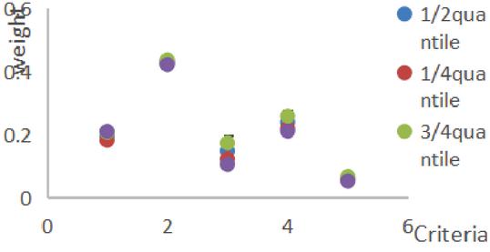
Figure 1 Optimal interval weights when using box-constraint.

In the Figure 1, The horizontal axis 1 to 5 are represented quality, price, comfort, safety and style respectively. When we find each standard weight interval, the raw data is only one of the values of the interval. The original data is not the optimal weight value in the interval. As shown in the Figure 1, it is more convincing when we take the quantile of the interval. We can have an optimal weight of all criteria as follow Figure 2.

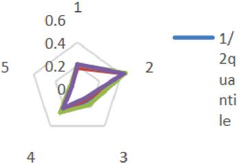
Figure 2 The rank of criteria weight under different quantile.

According to the Figure 2, the relative weight position of all criteria can be seem. Price and style are the most important and the least criteria respectively. The other criteria have a rank as quality $=$ safety $>$ comfort when we take the original method. If we use the new method, we can get a rank as: safety $>$ quality $>$ comfort.

When we take the interval of relative preference in Table 3 into model (12), we can get the optimal interval of weight through resolving the model (12), all interval are the range of weight. All criteria can get the only interval since the example is a full consistent problem.

$w_1=[0.1233,0.2194],w_2=[0.3316,0.4322],w_3=[0.0732,0.1354],$

$w_4=[0.1833,0.2594],w_5=[0.0321,0.1344]\mathit{\hspace{1em}}\text{and}\mathit{\hspace{1em}}\xi =0.$

Then we can take $QW$ value as weight for each criterion, and get the rank of all criteria in Figure 3.

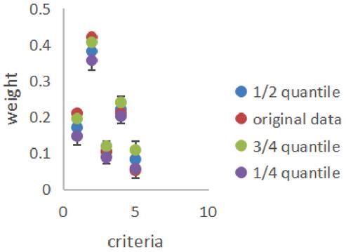
Figure 3 Optimal interval weights when using ellipsoidal-constraint.

As we can see from Figure 3, weight interval of each criteria can be achieved. The weight which we can get by using origin method are arbitrarily value in weight interval. So, it is not reasonable to take arbitrary value as optimal weight value. The rank of all criteria is price $>$ safety $=$ quality $>$ comfort $>$ style by original method. Safety and quality cannot be distinguished which is more important. But this problem can be resolve by using improved method, five criteria can be rank as price $>$ safety $>$ quality $>$ comfort $>$ style. It is rational for us take QW value as optimal weight. The rank of all criteria is more effective that we can see from Figure 4.

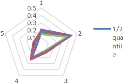
Figure 4 The rank of criteria weight under different quantile.

Example 2. Firstly, we take the interval of box-constraint preference into model (9), through solving the model (9) we can get $\xi =0.1324$. This result implies the problem is a non-full consistent, so we can get multiple optimal weight interval. All the optimal weight intervals are interval set as follow:

$w_1$	$=[(0.0879,0.1049),(0.2214,0.2301)];$
$w_2$	$=[(0.3831,0.4201),(0.4136,0.4689)];$
$w_3$	$=[(0.1042,0.1302),(0.2234,0.2321)];$
$w_4$	$=[(0.1421,0.1702),(0.1597,0.2053)];$
$w_5$	$=[(0.0311,0.1002),(0.0589,0.0932)];$

Through all weight interval sets above, we can take different quantile of interval. In this experience we take the middle of lower interval and upper interval as light and right limit of new weight interval. Then we also take different quantile as weight of all criteria. The result can be achieved from Figure 6. In the Figure 6, we know all the original data within interval. But all the weight values under different criteria have different positions in the interval. Therefore, it is unreason to take the original data as the optimal weighted value. The weight value obtained in the original method is not the optimal weight. For this problem of non-full consistency, we can obtain a set of interval weights, and it is more convincing to take the weight value of all the criteria through interval quantiles.

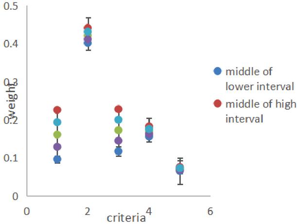
Figure 5 Optimal interval weights when using box-constraint.

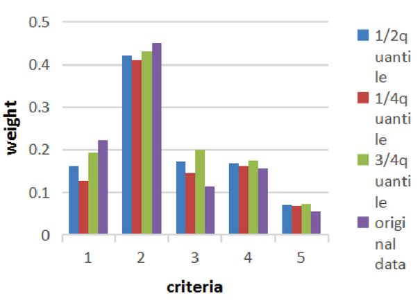
Figure 6 The rank of criteria weight under different quantile.

We can know according to Figure 6, we can see that all the original data are within the interval, but the position of data are scattered randomly within the interval and no rule, so the weight value found by the original method is only a set of feasible values and not the optimal value. In this paper, it is more convincing to take the value of the quantile position of all the intervals as the weight value. The original method finally ranked the 5 criteria as price $>$ quality $>$ safety $=$ comfort $>$ style. But we can get a new rank as price $>$ comfort $>$ quality $>$ safety $>$ style when we take ${\alpha }_{\frac{1}{2}}$, ${\alpha }_{\frac{3}{4}}$ and ${\alpha }_{\frac{1}{4}}$ of interval as we can see from Figure 6. In the original method, the weight cannot be compared between safety and comfort. The optimized approach has already shown its advantages. But to avoid the chance, a third set of data was compared.

Then we take the interval preference of ellipsoidal-constrained into model (12). We can get five sets of weight interval and $\xi$ as follow:

$w_1$	$=[(0.0321,0.0873),(0.1314,0.1677)];$
$w_2$	$=[(0.3841,0.4044),(0.4231,0.5821)];$
$w_3$	$=[(0.1321,0.1566),(0.1891,0.2054)];$
$w_4$	$=[(0.1631,0.1988),(0.2133,0.2431)];$
$w_5$	$=[(0.0145,0.1421),(0.1531,0.2003)];$
$\xi$	$=0.1247$

Since this case is non-full consistent problem, so we can get a set of weight interval for each criterion. Next, we take different QW as weight value in Figure 7.

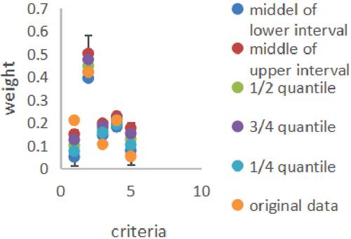
Figure 7 Optimal interval weights when using ellipsoidal-constraint.

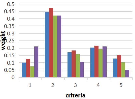
Figure 8 The rank of criteria weight under different quantile.

As we known from Figure 8, the green point is weight which can get from original method. The weight of first and third criteria are out of weight interval, so weight value are higher. It is not reasonable from this angle. We can get a rank of all criteria as price $>$ quality $>$ safety $>$ comfort $>$ style.

Example 3. Firstly, we can take the preference interval of second line into model (9), through solving the model (9) we can get $\xi =0.2435$ and multiple sets of weight interval as follow:

$w_1$	$=[(0.0768,0.0989),(0.1937,0.2264)];$
$w_2$	$=[(0.3728,0.3969),(0.4028,0.4345)];$
$w_3$	$=[(0.0978,0.1285),(0.1934,0.2169)];$
$w_4$	$=[(0.1397,0.1678),(0.1897,0.2064)];$
$w_5$	$=[(0.0437,0.0784),(0.0978,0.1253)];$

When we use ${\alpha }_{\frac{1}{2}}$ of interval sets as the right and left limit of new weight interval as follow:

$w_1$	$=[0.08785,0.22575],w_2=[0.38485,0.44125],$
$w_3$	$=[0.11315,0.22775],w_4=[0.15375,0.1825],$
$w_5$	$=[0.06105,0.07605]$

Then we use ${\alpha }_{\frac{1}{4}}$, ${\alpha }_{\frac{3}{4}}$, ${\alpha }_{\frac{1}{2}}$ of new weight interval, the result as in Figure 9.

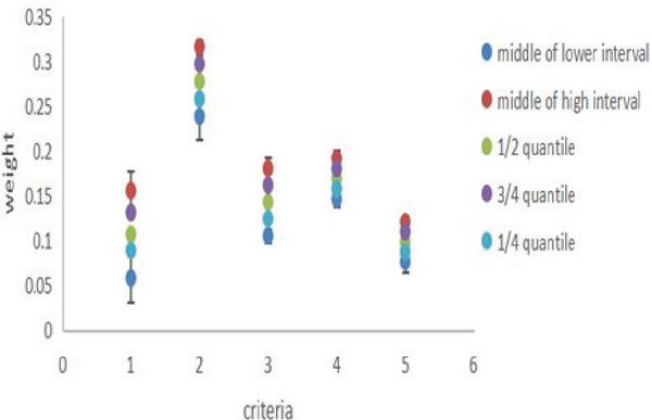
Figure 9 Optimal interval weights when using ellipsoidal-constraint.

Through Figure 9 we can know the rank of all criteria. The branches from 1 to 5 represent quality, price, comfort, safety, and style. When we take quantile of interval as weight, a consistent rank as price $>$ safety $>$ comfort$>$ quality $>$ style. However, the rank can be obtained as price $>$ quality $>$ safety $>$ comfort $>$ style by original method. Since the weight value of each criteria is irregular. So, the rank of all criteria is not reasonable.

6 Conclusion

In this paper, the fix relative preference value in the original method is changed into the weight interval, and the left and right limits of weight interval are substituted into the model respectively, so that the weight interval of each standard can be calculated. After improvement, the value obtained through the model is no longer a unique value but the feasible region of weight value. The position of selected optimal value in the interval can be clearly seen through the feasible region of the weight, and it is more reasonable to take the value on the fixed quantile as the weight value. This paper have three advantages as follow: 1. this paper can calculate the weight feasible region of each criterion. 2. The position of optimal value in the feasible interval can be seem clearly, which is more intuitive. 3. Each criterion can be sorted according to the overall position of weight value through the feasible region of weight, which is more reasonable.

In this paper, we use box-constraint and ellipsoidal-constraint of robust optimization to improve the best-worst multi-criteria decision-making method, we can also use other constraint forms to improve the relative preference value.

References

[1] M.V. Kumar, M. Ramkumar, S. Digjoy. A Multi-Criteria Decision-Making Approach for the Urban Renewal in Southern India. Sustainable Cities and Society, 42(2018), 471–481.

[2] C.J. Li, M. Negnevitsky, X. Wang, W. Yue, X. Zou. Multi-criteria analysis of policies for implementing clean energy vehicles in China. Energy Policy, 34(2019), 826–840.

[3] G. Tré, R. De Mol, A. Bronselaer. Handling veracity in multi-criteria decision-making: A multi-dimensional approach. Information Sciences, 65(2018), 541–554.

[4] X. Gou, Z. Xu, H. Liao et al. Multiple Criteria Decision Making based on Distance and Similarity Measures under Double Hierarchy Hesitant Fuzzy Linguistic environment. Computers & Industrial Engineering, 35(2018), 516–530.

[5] R. Jafer Best-Worst Multi-Criteria Decision-Making Method. Omega, 53(2015), 49–57.

[6] Q. Mou, Z. Xu, H. Liao, et al. An intuitionistic fuzzy multiplicative best-worst method for multi-criteria group decision making. Information Sciences, 374(2016), 224–239.

[7] S. Guo, H. Zhao. Fuzzy best-worst multi-criteria decision-making method and its applications. Knowledge-Based Systems, 32(2017), 23–31.

[8] H. Martin, G. Marc, W. Michael. A largest empty hypersphere metaheuristic for robust optimization with implementation uncertainty. Computers & Operations Research, 65(2019), 64–80.

[9] M. Kaedi, C. Ahn. Robust Optimization Using Bayesian Optimization Algorithm: Early Detection of Non-robust Solutions. Applied Soft Computing, 121(2017), 1125–1138.

[10] L. Marla, V. Vaze, C. Barnhart. Robust Optimization: Lessons Learned from Aircraft Routing. Social Science Electronic Publishing, 55(2017), 165–184.

[11] R. Jafar. Best-worst multi-criteria decision-making method: Some properties and a linear model. Omega, 44(2016), 126–130.

Biographies

Deqiang Qu is a Ph.D. Student of the Business School at University of Shanghai for Science and Technology. His current research interests include: Decision making under uncertain.

Zhong Wu received the Ph.D. degree from Tongji University, China. He is now the Vice President of University of Shanghai for Science and Technology. His current research interests include: Decision making under uncertain, game theory, and public management.

Shaojian Qu received the Ph.D. degree from Xi’an Jiaotong University, China, and was a Research Fellow at National University of Shanghai for 4.5 years. He is now a Professor of the Business School at University of Shanghai for Science and Technology. His current research interests include: Decision making, game theory, supply chain management, and portfolio.

Fan Zhang is a master student at the University of Shanghai for Science and Technology since autumn 2017. His main research directions in school are crowdfunding, multi-cirteira decision and robust optimization. He has published two papers during the academic year.

Ping Li is a master’s degree candidate in management science and engineering at the University of Shanghai for Science and Technology. His current research interests include: multi-attribute decision making, intuitionistic fuzzy theory and emergency management. During master’s studies, he has published two academic papers.

Journal of Web Engineering, Vol. 19_7-8, 1067–1088.
doi: 10.13052/jwe1540-9589.19787
© 2020 River Publishers

Abstract

1 Introduction

2 Best-Worst Multi-criteria Decision-making Method

3 Robust Optimization

3.1 Uncertainty in Relative Preference

3.2 The Best-worst Multi-criteria Decision-making Method in Box-constraint

3.3 The Best-worst Multi-criteria Decision-making Method in Ellipsoidal-constraint

4 Analysis of Non-full and Full Consistent Problems

4.1 Analysis of Weight Interval

5 Numerical Examples

6 Conclusion

References

Biographies