An Application of CHNN for FANETs Routing Optimization

Xing Wei^1,2 and Hua Yang^2,*

¹School of Computer Science and Information Technology, Guangxi Normal University, 541004, Guilin, China

²Guilin University of Aerospace Technology, 541004, Guilin, China

E-mail: gl-yh@guat.edu.cn

*Corresponding Author

Received 15 September 2020; Accepted 21 October 2020; Publication 11 December 2020

Abstract

Routing algorithm has a decisive influence on routing quality, and routing quality has a direct impact on network performance. For FANETs, the highly dynamically changing topology poses a challenge to the design of routing algorithms. The paper studies the characteristics of FANETs, and uses a CHNN to search for FANETs routing to form CHNNR. Using NS3 as a simulation tool, a highly dynamic simulation scheme in the background of the network topology of the air flight platform was designed, making the simulation scene closer to the dynamic performance of the FANETs highly dynamic mobile node. By comparing parameters such as network delay, normalized network throughput, routing load and data transmission success rate, the performance of CHNNR and passive routing algorithms is analyzed and compared. The simulation results show that the comprehensive performance of CHNNR is better than other passive routing algorithms, and it is more suitable for FANETs networks where nodes move at a high speed and the network topology changes frequently, and lay the foundation for the next research.

Keywords: Flying ad hoc network, routing algorithm, neural network,. Hopfiled neural network.

1 Introduction

As a special MANETs, FANETs is widely used in military, agriculture, disaster search and rescue and other fields with the characteristics of no center, self-organization, and self-healing [1–5]. Due to the characteristics of FANETs, such as limited bandwidth, limited node energy, and strong node mobility, designing an effective and reliable routing algorithm is a very challenging problem [6, 7]. On the one hand, the feasible path between network communication nodes is an unknown variable. In this case, the solution space includes all loop-free network paths. In larger FANETs, there may be too many such paths. So that it is impossible to search for a feasible solution space in an exhaustive manner. On the other hand, there is currently no specific routing algorithm specifically for FANETs. Most MANETs routing algorithms only use the number of hops as a measurement. It may be difficult for FANETs to achieve effective resource utilization or execute critical real-time applications. Therefore, consider using an artificial intelligence algorithm to search for FANETs routing, and at the same time add restrictions on routing stability, routing maximum power, and maximum available bandwidth to the searched routing. The Hopfiled neural network is just such a suitable artificial intelligence method, because it can ensure that the solution converges to the minimum of the energy function, although it cannot ensure that the global minimum is reached.

2 Related Works

2.1 Routing Algorithm

The routing algorithm is a technology that determines how form a routing table and plans routes for data packet forwarding based on the routing table. The routing table maintains information about connected nodes, new access nodes, and neighbor nodes so that the source node can send data to the destination node. Generally, routing algorithms are divided into three different categories according to the nature and attributes of routing: active routing algorithms, reactive routing algorithms and hybrid routing algorithms [8].

The active routing algorithm regularly checks and maintains the complete routing information of the routing. Therefore, every time a node sends a data packet before routing information has been planned, all nodes in all networks must constantly maintain one or more routing tables to adapt to the constantly changing network topology, thereby ensuring that the data is between task nodes in the network transfer. The main representative routing algorithms is: OLSR [9, 10], TBRPF [11, 12], DSDV [13, 14] etc. The reactive routing algorithm only performs the route discovery process when the node needs it, and follows the route discovery and route maintenance operations. After the route is established, the data are transmitted through the marked path. The main representative routing algorithms is: DSR [15, 16], AODV [16, 17], etc. Hybrid routing algorithm is a combination of active routing algorithm and passive routing algorithm. This type of algorithm subdivides nodes into different groups and uses active routing to maintain the routing table within each different group. Passive routing is used between groups. Through hybrid routing algorithms, the network can be in active routing algorithms. Switch between and passive routing algorithms. The foremost representative algorithms are: ZRP [18, 19], and so on.

Reactive routing algorithm needs to send out control packets for information exchange when searching for routes,. Its delay will be higher than that of active routing. However, in networks with frequent topological changes such as FANETs, it is too expensive to periodically check and maintain complete routing information. Therefore, in FANETs routing design, this paper basically consider reactive routing algorithms.

2.2 Hopfiled Neural Network

Hopfield neural network [20–23] is a single-layer symmetrical full-feedback neural network, which is very suitable for solving combinatorial optimization problems, and has received extensive attention for its simplicity and representativeness. FANETs routing lookup problem can be regarded as an optimization problem with constraints. And Hopfield neural network is very suitable for solving such problems. At the same time, the calculation of the Hopfield neural network adopts a parallel processing method. Its calculation amount will do not increase exponentially with the increase of the dimensionality of neurons. This is especially important for FANETs network, because the energy of nodes in the network is always limited, which means that the energy of network nodes will not consume more. The Hopfield neural network can be divided into continuous type and discrete type according to the type of input and output variables. The corresponding neuron and the mathematical model of the system can be described by differential equations and nonlinear differential equations. For FANETs routing search problems, this article uses CHNN to search.

The Hopfield neural network first proposed the concept of energy function. Its main idea to solve the combinatorial optimization problem is: express each state value of the neural network with the corresponding variable in the optimization problem, and then construct the objective function of the optimization problem, and the objective function And all the constraints of the problem are constructed as the energy function of the neural network after the integration of the penalty function, and then according to the principle of the neural network, the partial derivative of the energy function about the neuron output is obtained, and the obtained expression is the neural network Kinetic equations. According to the energy function and dynamic equation of the network, a complete neural network model can be assigned. When the energy function tends to a stable minimum with iteration, the network state obtained is the optimal solution to the optimization problem. The general steps are as following:

1. For the combinatorial optimization problem to be processed, select an appropriate method to represent the value of each variable, so that the solution of the problem corresponds to the output of the neural network one by one;

2. Construct the energy function E of the neural network, and use the minimum value of the energy function to represent the optimal solution of the problem, that is, when the value of the energy function tends to the minimum and the network is stable, the result obtained is the solution of the optimization problem;

3. Determine the number of neurons and the structure of the neural network according to the energy function E;

4. Establish a neural network according to the network structure. Begin the network and make it reach a stable state after a certain number of iterations. At this time, the output of the network is the optimal solution to the problem under certain conditions.

3 Optimization Method

3.1 Some Functions

Set FANET as an undirected graph $G = (V, E)$ , where $V = (1, 2, \dots, n)$ is the node in the FANET network, and $E$ is the road section of adjacent nodes. The corresponding weights of each road segment in the network are $C_{i j}^{m}$ , where $m = 1, 2, \dots, M, i = 1, 2, \dots, n, j = 1, 2, \dots, n$ . The function is as follows function (1). Among them, $L S_{i j}$ is expressed as the stability prediction of the link between nodes $i$ and $j$ . $P_{i}$ and $P_{j}$ represents the energy of node i and node j, $B_{i j}$ represents the bandwidth of the link between node $i$ and node $j$ . $ω$ represents the importance of the link weight between nodes and $ω_{1} + ω_{2} + ω_{3} = 1$ . In the mobile prediction model, the free-space ropagation model is adopted, the received signal

C_{i j} = ω_{1} L S_{i j} + ω_{2} (P_{i} + P_{j}) + ω_{3} B_{i j}

(1)

strength only depends on the distance between the receiver and the transmitter, and the clocks of all network nodes are synchronized, such as the network time protocol (NTP) or Global Positioning System (GPS) clock. If the movement parameters of two adjacent nodes are known, such as flight speed, horizontal flight direction, wireless signal transmission distance, etc., the length of time that the links of the two adjacent nodes are maintained can be determined. If nodes i and j are in each other’s transmission coverage r, the position, speed, and direction of node i are expressed as $(x_{i}, y_{i}, z_{i})$ , $v_{i}$ , $θ_{i}$ , and the position, speed, and direction of node j $(x_{j}, y_{j}, z_{j})$ , $v_{j}$ , $θ_{j}$ , in order to simplify the calculation, the default flight altitude is at the same level, then the time that the link between node i and node j remains stable is predicted as:

L S_{i j} = \frac{- (a b + c d) + \sqrt{(a^{2} + c^{2}) \cdot r^{2} - {(a d - b c)}^{2}}}{a^{2} + c^{2}}

(2)

Among them, $a = v_{i} c o s θ_{i} - v_{j} c o s θ_{j}$ , $b = x_{i} - x_{j}$ , $c = v_{i} s i n θ_{i} - v_{j} s i n θ_{j}$ , $d = y_{i} - y_{j}$ . When $v_{i} = v_{j}$ and $θ_{i} = θ_{j}$ , that is, when the flight speed and flight direction of adjacent nodes are the same, the two adjacent nodes can be regarded as static nodes with the highest stability, that is, $L S_{i j} = \infty$ .

3.2 Objective Function

The FANETs route selection problem can be formulated as an optimization problem, that is, as a solution to system equations and inequalities, the constraints that form the problem maximize or minimize an objective function on a set of unknown variables. If the FANETs path selection problem is linked with the energy function of CHNN, it is necessary to transform the constrained problem into an unconstrained problem, and then into an energy function. For the treatment of constraint conditions, the commonly used method is penalty function, including external electrical method, interior point method, multiplier method, etc., using the idea of penalty function to add constraint conditions to the objective function.

3.3 Energy Function

The FANETs routing optimization model is linked with the Hopfield neural network, and the energy function of the network is constructed according to the optimization objectives and constraints of the optimization model. Therefore, the energy function of FANETs routing optimization can be defined as follows:

Among them, if there is a route between node i and node j, then $γ_{i j} = 1$ , if there is no route, then $γ_{i j} = 0$ . The first term of the energy function is the objective function of the routing optimization problem, that is, the value of the weighted sum of each objective; $α_{1}$ is used to constrain non-existent paths so that they cannot exist in the optimal path; $α_{2}$ , $α_{3}$ make node s and node d in the result, that is, to ensure that the source node and destination node are included in the optimal path; $α_{4}$ transforms the 0–1 constraint into a value that can be applied by CHNN; $α_{5}$ ensures that node d reaches 1 when there is a route between nodes s.

$E$	$= \sum_{m = 1}^{m} \frac{P}{2} {(\sum_{i, j} C_{i j}^{m} x_{i j} - m)}^{2} + α_{1} \sum_{i = 1}^{n} \sum_{j = 1}^{n} γ_{i j} x_{i j} + α_{2} {(\sum_{j = 1}^{n} x_{j d} - 1)}^{2}$
	$+ α_{3} {(\sum_{j = 1}^{n} x_{s j} - 1)}^{2} + α_{4} \sum_{i = 1}^{n} \sum_{j = 1}^{n} x_{i j} (1 - x_{i j}) + α_{5} (1 - x_{d s})$	(3)

3.4 Matrix Dimension Conversion

FANETs, the energy of nodes is limited, so it is necessary to convert high-dimensional matrices into low-dimensional matrices to improve computing efficiency and reduce node energy consumption. Because the road network and weight matrix in the energy function are both two-dimensional at this time, they need to be converted to vectors to represent them, that is, the matrixes need to be expanded in order and converted to vectors to represent them. Therefore, here this paper use the vector element $x_{k}$ to replace the element $x_{i j}$ in the two-dimensional matrix, where $k = 1, 2, \dots, n^{2}$ , and the relationship between $x_{k}$ and $x_{i j}$ is as follows:

k = n (i - 1) + j

(4)

Therefore, the energy function is rewritten into the following form:

$E$	$= \sum_{m = 1}^{M} \frac{P}{2} {(\sum_{k} C_{k}^{m} x_{k} - m)}^{2} + α_{1} \sum_{k = 1}^{n^{2}} γ_{k} \cdot x_{k} + α_{2} {(\sum_{i = d}^{n (n - 1) + d} x_{k} - 1)}^{2}$
	$+ α_{3} {(\sum_{I = n (s - 1) + 1}^{n s} x_{k} - 1)}^{2} + α_{4} \sum_{k = 1}^{n^{2}} x_{k} (1 - x_{k})$
	$+ α_{5} (1 - x_{n (d - 1) + s})$	(5)

3.5 Iterative Equation

According to the form of the energy function and the nature of CHNN, can get:

$\frac{\partial E}{\partial x_{l}}$	$= \sum_{m = 1}^{M} P C_{i}^{m} (\sum_{k = 1}^{n^{2}} C_{k}^{m} x_{k} - m) + α_{1} γ_{l}$
	$+ 2 α_{2} S_{l - d} S_{n (n - 1) + d - l} (\sum_{k = d}^{n (n - 1) + d} x_{k} - 1)$
	$+ 2 α_{3} S_{1 - n (s - 1) - 1} S_{n s - l} (\sum_{k = n (s - 1) + 1}^{n s} x_{k} - 1)$
	$+ α_{4} (1 - 2 x_{l}) - α_{5} S_{l - n (d - 1) - s} S_{n (d - 1) + s - l}$	(6)
$\frac{\partial^{2} E}{\partial x_{k} \partial x_{l}}$	$= \sum_{m = 1}^{m} P C_{l}^{m} C_{k}^{m} + 2 α_{2} S_{l - d} S_{n (n - 1) + d - l} S_{k - d} S_{n (n - 1) + d - k}$
	$+ 2 α_{3} S_{l - n (s - 1) - 1} S_{n s - 1} S_{k - n (s - 1)}$
	$S_{n s - k} - 2 α_{4} S_{k - 1} S_{l - k}$	(7)

The definition of the S function is:

S_{i n d e x} = {\begin{matrix} 0 & i n d e x < 0 \\ 1 & i n d e x \geq 0 \end{matrix}

(8)

The connection weight of the neuron can be obtained as:

w_{u} = - \frac{\partial^{2} E}{\partial x_{k} \partial x_{l}}

(9)

The bias of each neuron is:

$I_{l} = - \frac{\partial E}{\partial x_{l}} (0)$	$= \sum_{m = 1}^{M} P C_{l}^{m} m - α_{1} γ_{l} + 2 α_{2} S_{l - d} S_{n (n - 1) + d - l}$
	$+ 2 α_{3} S_{l - n (s - 1)} S_{n s - l} - α_{4} + α_{5} S_{l - n (d - 1) + s} S_{n (d - 1) + s - l}$	(10)

So far, the main parameters of CHNN for finding FANETs optimized routing have been obtained. The main connection weights $W$ and offset $I$ are only related to the weights $C$ , $P$ , $α$ , $S_{i n d e x}$ , etc. of the road section.

4 CHNN Routing Algorithm

Use CHNN to optimize FANETs routing, and named it CHNNR, adopts reactive routing algorithm, starts the route discovery process on demand according to communication requirements, and establishes route table and neighbor table on demand to reduce overhead and save network bandwidth resources. In this article, the routing table is established using the CHNN algorithm. The format is shown in Table 1, which mainly includes Destination Node, Source Node, In node, Out node, Build Date, and Stability Time.

Table 1 Route table

Destination Node	Source Node	In node	Out node	Build Date	Stability Time
N $_{d}$	N $_{s}$	N $_{i}$	N $_{o}$	aa:bb:cc:dd	x
…

In this article, use an improved HELLO packet to perform topological exchange on neighboring nodes to inform neighboring nodes of their own node’s existence and attributes. The improved HELLO packet contains information such as node bandwidth, node flight speed, node location, and node flight direction. Each neighbor node that receives HELLO pakcet checks and updates its Neighbor table so that it can be used to calculate the routing weight between neighboring nodes when needed, and use CHNN to search for optimized routes. The format of Neighbor table is shown in Table 2.

Table 2 Neighbor table

Neighbor Node	Bandwidth	Flying speed	Flying direction	Position
Na	$B_{a}$	$v_{a}$	$θ_{a}$	$(x_{a}, y_{a}, z_{a})$
Nb	$B_{b}$	$v_{b}$	$θ_{b}$	$(x_{b}, y_{b}, z_{b})$
…

4.1 Route Discovery

The route search process first need to calculate the route weight between adjacent nodes, which are realized by the interaction of adjacent nodes on the route. When the information exchange between neighboring nodes is completed, the CHNN algorithm is started to search for optimized routes to build a routing table. When a node decides that it needs a route to reach a destination node, if the node did not know the destination node before, or a valid route to the destination node has become an invalid route or the stability has expired, then the node needs to be started Route lookup process. When a route is needed for communication, the source node first checks its own routing table, and if there is a route to the node, it checks the establishment date and stable time of the route entry. If the interval between the creation date of the route entry and the current date exceeds the stable time, the routing table considers this route as an invalid route and deletes the route and starts the route search process. If the source node does not know the destination node before, it will first send a HELLO packet to the neighbor node, update the Neighbor table according to the HELLO packet returned by the neighbor node, calculate the routing weight between neighboring nodes based on the updated neighbor table, and use CHNN to optimize routing Find and update the route table, and then send data according to the route table.

4.2 Route Maintain

In CHNNR, there is no need to reserve a backup route, because the maintenance of the backup route will generate new network overhead. For a specific route application, only one route is selected and only one route is valid. Not using alternate routes means that periodic route updates are not required, which can effectively save network energy. If the source node has a route break, the route discovery process is directly started for route search. When the route breaks in the intermediate node, the node broadcasts the HELLO packet to the neighbor node. The neighbor node that receives the HELLO packet performs local routing update and routing maintenance.

5 Simulation and Discuss

5.1 Performance

In multi-hop ad hoc networks such as FANETs, the main parameters that affect network performance are [23, 24]:

• Packet delivery ratio (PDR): PDR is the ratio of the data packet $P_{s}$ sent by the application layer of the source node to the data packet $P_{r}$ received by the target node, that is, the statistical measure of the correct transmission of the data packet. It reflects the two main characteristics of FANETs network reliability and network congestion. The function is shown in function (11).

P D R = \frac{P_{r}}{P_{s}}

(11)

• Throughput (TH): TH is the amount of data transmitted from source to destination per unit time, which can be divided into node throughput and network throughput. Node throughput is the data packet received by the target node per unit time, and network throughput is the network throughput per unit time. The average value of the sum of data packets received by all nodes.

• Delay (DE): DE is the time required for a data packet to be sent from the source to the destination for correct transmission, including the sum of all delays such as queuing delay, processing delay, and sending delay. Usually, take the average value, which is the average delay.

• Normalized routing load: Under different network loads, the transmission volume of routing control packets per unit time. Reflects the rate at which the network topology changes.

5.2 Parameter Settings for NS3

In order to verify the effectiveness of the CHNNR algorithm and improve the performance of FANETs, this paper developed a CHNN algorithm based on C++. First, the effectiveness of CHNN on routing optimization was verified on the PC, and then it was transplanted to NS3 [25, 26] for simulation verification. NS3 is a major new and improved version of NS2. The realization of NS3 simulation model relies on C++, and its core design is extensible to support future development. NS3 also supports integration with actual equipment.

In the NS3 simulation environment, the main parameter settings are shown in Table 3. In the simulation scenario, 50 nodes are distributed in the area of 500 m $\times$ 500 m, the simulation time is set to 900s. FANETs node Channel uses wireless channel, bandwidth is 11mbps, physical layer uses 802.11 DCF, network layer uses CHNNR, AODV and DSR, node mobility model uses Random waypoint mobility [27–29], CBR Connections is set to 20.

Table 3 Parameters of simulation environments

Parameters	Value
Simulator	NS3
Number of nodes	50
Simulation range	500 m $\times$ 500 m
Channel type	Wireless channel
Channel bandwidth	11 Mbps
MAC layer	802.11 DCF
Network layer	CHNNR, AODV, DSR
Transfer Models	WaveLan
Mobility model	Random waypoint mobility
Data transmission rate	1 Mbps
CBR Connections	20
Simulation times	900 $s$

5.3 Results and Discuss

Because the energy of a single aircraft is limited, in order to save energy as much as possible, routing optimization algorithms are required to converge quickly. Specifically in the CHNN search for optimized routing, it needs to converge to the stable state of the neural network in a limited number of cycles. In order to verify the convergence speed of CHNN in routing optimization, we deliberately first simulated and ran the routing optimization CHNN algorithm on PC. The scale of nodes in the network is 50, and the weights between nodes are set randomly. limiting the number of cycles of the CHNN algorithm to no more than 10,000. The results of running on an ordinary PC show that the average time to find the optimized route is about 800ms, and the average number of cycles is 2000. Therefore, it can be directly transplanted to the flying ad hoc network.

After confirming the feasibility and effectiveness of the CHNN algorithm, we transplanted the CHNN algorithm based on NS3. According to the setting in the paper [21–24], in the CHNN algorithm, $P = 500$ , $α_{1} = α_{2} = α_{3} = α_{4} = α_{5} = 200$ . In the NS3 simulation, we focused on comparing the Packet Delivery ratio, delay, and delay of the three routing protocols of CHNNR, DSR, and AODV. Key performance indicators such as the packet delivery ratio, the throughput and the delay. The detailed comparison is shown in Figures 1–3.

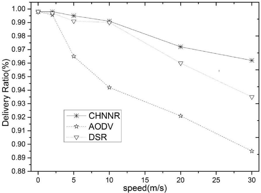
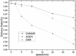
Figure 1 The packet delivery ratio when node mobility speed increase.

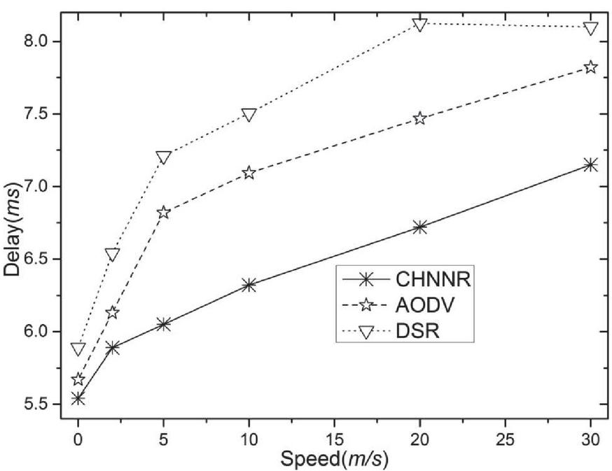
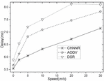
Figure 2 The average delay when node mobility speed increase.

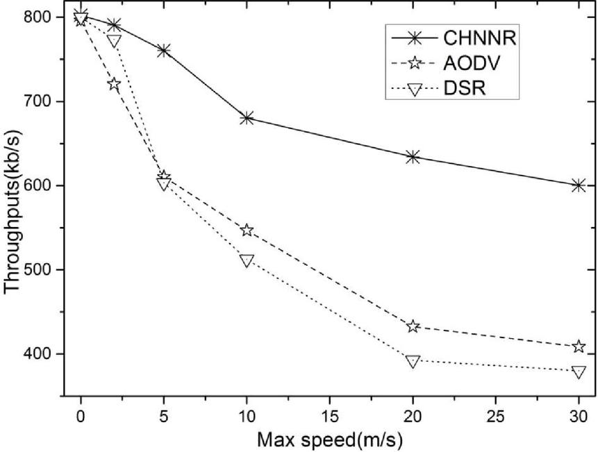
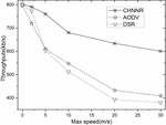
Figure 3 The throughputs when node mobility speed increase.

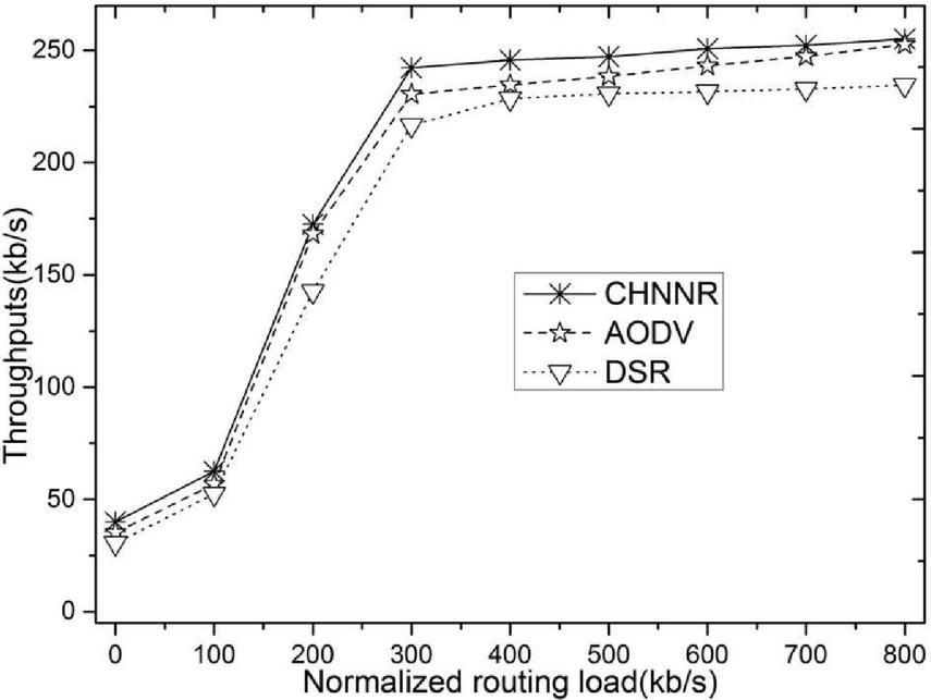
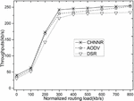
Figure 4 The normalized routing load.

When the node moving speed is low, the probability of routing breakage in the network is small, so the network load is also low. At this time, the network throughput under several routing metrics is not much different. As the moving speed of nodes increases, the possibility of routing breaks in the network increases, and the Route discovery process of nodes with communication requirements is also frequently started. At this time, the control packets in the network will inevitably increase. With the continuous increase of network load, local network congestion has gradually increased. CHNNR can avoid areas with intense competition and conflict through reasonable routing, and can alleviate the increase in network congestion. The route selected by CHNNR takes into account various factors of the node, which can reduce the number of packet transmissions, thereby reducing the average end-to-end delay (show in Figure 2), increasing the packet arrival rate (show in Figure 1), and reducing the number of nodes Power consumption extends the life of the node, thereby increasing the throughput of the network (show in Figure 3).

Select high-speed mobile scenes and compare CHNNR, DSR and AODV under fair conditions. Using a network model of 50 nodes, the number of communication source nodes is fixed at 20. The packet transmission rate slowly increases, knowing where the throughput is saturated. The throughput here represents the sum of the receiving throughput of the destination node of each data source node, and the “network load” the sum of the sending rates of all data source nodes, in kb/s. If there is no retransmission, then the ratio of throughput to network load is equal to the packet delivery rate.

Since the HELLO packet uses an extended control format for cross-network layer information exchange, the length of the control packet becomes larger. Show in Figure 4, we can see that the routing load of CHNNR is higher than that of AODV and DSR. However, considering the impact of CHNNR on network throughput, the improvement of network key performance indicators such as average delay and packet arrival rate is within an acceptable range.

6 Conclusions

Based on careful study of the traditional active routing AODV and DSR in MANETs, this paper proposes an optimized routing algorithm CHNNR based on CHNN and applies it to FANETs. CHNNR comprehensively considers the energy and bandwidth of the node, and establishes an optimized route between the source node and the destination node. The simulation results show that CHNNR can alleviate network congestion, reduce node power consumption, extend node life, and improve the life cycle of FANETs. However, the simulation environment setting in this article is more ideal, without considering more scenarios and influencing factors of FANETs, the next step can be an engineering test on CHNNR to verify its reliability.

Acknowledgements

This work is partially supported by the project for Natural Science Foundation of GuangXi (2020GXNSFAA159094); High level Innovation team of Guangxi Colleges and Universities-Intelligent Information Technology and UAV Application; The Science and Technology Research Project of Department of Education of Guangxi (2019KY0815).

References

[1] S. B. Amarat, P. Zong, 3D path planning, routing algorithms and routing protocols for unmanned air vehicles: a review, Aircraft Engineering and Aerospace Technology, (2019) 1–11.

[2] E. Cruz, A Comprehensive Survey in Towards to Future FANETs, IEEE Latin America Transactions, 16(3) (2018) 876–884.

[3] I. Bekmezci, O. K. Sahingoz, Ş. Temel, Flying ad-hoc networks (FANETs): A survey, Ad Hoc Networks, 11(3) (2013) 1254–1270.

[4] O. K. Sahingoz, Networking models in flying ad-hoc networks (FANETs): Concepts and challenges, Journal of Intelligent & Robotic Systems, 74(1–2) (2014) 513–527.

[5] H. Yang, Z. Liu,. An optimization routing protocol for FANETs, EURASIP Journal on Wireless Communications and Networking, 1 (2019) 1–8.

[6] Z. Zheng, A. K. Sangaiah, T. Wang, Adaptive communication protocols in flying ad hoc network, IEEE Communications Magazine 56.1 (2018): 136–142.

[7] A. Nadeem, T. Alghamdi, A. Yawar, A review and classification of flying Ad-Hoc network (FANET) routing strategies. Journal of Basic and Applied Scientific Research 8.3 (2018): 1–8.

[8] R. Sharma, T. Sharma, A. Kalia, A comparative review on routing protocols in MANET, International Journal of Computer Applications 133.1 (2016): 33–38.

[9] T. Clausen, P. Jacquet, C. Adjih, A. Laouiti, P. Minet, , P. Muhlethaler, L. Viennot,. Optimized link state routing protocol (OLSR), (2003).

[10] B. S. Kim, B. S. Roh, J. H. Ham,Extended OLSR and AODV based on multi-criteria decision making method., Telecommunication Systems 73.2 (2020): 241–257.

[11] R. Ogier, F. Templin, M. Lewis, Topology dissemination based on reverse-path forwarding (TBRPF) (2004), IETF RFC 3684.

[12] M. Sana, and L. Noureddine, Multi-hop energy-efficient routing protocol based on Minimum Spanning Tree for anisotropic Wireless Sensor Networks, International Conference on Advanced Systems and Emergent Technologies (2019), pp. 209–214.

[13] C. E. Perkins, P. Bhagwat, Highly dynamic destination-sequenced distance-vector routing (DSDV) for mobile computers, ACM SIGCOMM computer communication review, 24(4) (1994) 234–244.

[14] N. Wang, R. Datla, and H. Jhajj. NCMDSDV: A Neighbor Coverage Multipsth DSDV Routing Protocol for MANETs, 11th International Conference on Communication Software and Networks (2019), pp. 46–50.

[15] D. B. Johnson, D. A. Maltz, J. Broch, DSR: The dynamic source routing protocol for multi-hop wireless ad hoc networks, Ad hoc networking, 5 (2001) 139–172.

[16] H. Yang, Z. Li, Z. Liu, A method of routing optimization using CHNN in MANET, Journal of Ambient Intelligence and Humanized Computing, 10(5) (2019) 1759–1768.

[17] C. Perkins, E. Belding-Royer, S. Das, Ad hoc on-demand distance vector (AODV) routing (2003) , IETF RFC 3561.

[18] H. Yang, Z. Li, Z. Liu, Neural networks for MANET AODV: an optimization approach, Cluster Computing, 20(4) (2017) 3369–3377.

[19] N. Beijar, Zone routing protocol (ZRP), Networking Laboratory, Helsinki University of Technology, Finland 9 (2002): 1–12.

[20] R. Gasmi, M. Aliouat, H. Seba, A Stable Link Based Zone Routing Protocol (SL-ZRP) for Internet of Vehicles Environment, Wireless Personal Communications (2020): 1–16.

[21] J. J. Hopfield, Neural networks and physical systems with emergent collective computational abilities, Proceedings of the national academy of sciences 79.8 (1982): 2554–2558.

[22] S. Zhang, Y. Yu, Q. Wang, Stability analysis of fractional-order Hopfield neural networks with discontinuous activation functions. Neurocomputing 171 (2016): 1075–1084.

[23] B. Bao, C. Chen, H. Bao, X. Zhang, Q. Xu, M. Chen, Dynamical effects of neuron activation gradient on Hopfield neural network: Numerical analyses and hardware experiments, International Journal of Bifurcation and Chaos, 29 (04) (2019): 1930010.

[24] K. Rajagopal, M. Tuna, A. Karthikeyan, İ. Koyuncu, P. Duraisamy, A. Akgul, Dynamical analysis, sliding mode synchronization of a fractional-order memristor Hopfield neural network with parameter uncertainties and its non-fractional-order FPGA implementation, The European Physical Journal Special Topics, 228.10 (2019): 2065–2080.

[25] P. Rajankumar, P. Nimisha, P. Kamboj, A comparative study and simulation of AODV MANET routing protocol in NS2 & NS3, International Conference on Computing for Sustainable Global Development (2014), pp. 889–894.

[26] http://www.nsnam.org

[27] F. Maan, N. Mazhar, MANET routing protocols vs mobility models: A performance evaluation, Third International Conference on Ubiquitous and Future Networks (2011), pp. 179–184.

[28] A. Bujari, C. E. Palazzi, D. Ronzani, FANET application scenarios and mobility models, The 3rd Workshop on Micro Aerial Vehicle Networks, Systems, and Applications (2017), pp. 43–46.

[29] K. Kumari, B. Sah, S. Maakar, S., A survey: different mobility model for FANET, International Journal of Advanced Research in Computer Science and Software Engineering, 5(6) (2015).

Biographies

Xing Wei, He received M. S. degree in Computer Science from Guilin university of electronic technology, Guilin, China, in 2011.He is currently professor of Guilin university of Aerospace Technology, Guilin, China. His main research interest is the application of artificial intelligence.

Hua Yang, He received M. S. degree in Computer Science from Guangxi normal university, Guilin, China, in 2011.He is currently professor of Guilin university of Aerospace Technology, Guilin, China. His main research interests are MANET and protocol simulation