Research on Network Security Situation Assessment and Forecasting Technology
Hongbin Wang1, Dongmei Zhao1, 2, * and Xixi Li2
1College of Computer and Cyber Security, Hebei Normal University, Shijiazhuang, China
2Hebei Key Laboratory of Network and Information Security, Shijiazhuang, China
E-mail: dmzhao@hebtu.edu.cn
*Corresponding Author
Received 17 September 2020; Accepted 27 October 2020; Publication 26 December 2020
Abstract
In recent years, the network security issues have become more prominent, and traditional network security protection technologies have been unable to meet the needs. To solve this problem, this paper improves and optimizes the existing methods, and proposed a set of network security situation assessment and prediction methods. First, the cross-layer particle swarm optimization with adaptive mutation (AMCPSO) algorithm proposed in this paper is combined with the traditional D-S evidence theory to evaluate the current network security situation; Then, the parameters and structure of traditional RBF neural network are optimized by introducing FCM (fuzzy c-means), HHGA (hybrid hierarchy genetic algorithm) and least square method. According to the optimized RBF neural network and situation assessment results, the next stage of network security situation is predicted. Finally, the effectiveness of the network security situation assessment and prediction method proposed in this paper is verified by simulation experiments. The algorithm in this paper improves the accuracy of situation assessment and prediction, and has certain reference significance for the research of network security.
Keywords: Network security situation, particle swarm optimization, D-S evidence theory, RBF neural network.
1 Introduction
As the complexity and unpredictability of the network are becoming increasingly apparent, and network security issues are increasing. In order to effectively prevent and control complex and changeable network security, many scholars and researchers have begun to study various security defense methods and technologies, so that they can grasp the current network operating status as a whole, sense the threats facing the current network environment in real time, and prediction of the future security trends, providing a reliable basis for network administrators to make timely and accurate security decisions [1].
In 1999, Tim bass first proposed the concept of network security situational awareness. In subsequent research, he also proposed a network security situational awareness framework based on multi-sensor data fusion [2]. In 2004, the Lawrence Berkeley National Laboratory in the United States developed the “potential threat of rotating cubes” system [3]. This system is very innovative in the field of network security, in which network traffic is expressed using points. In 2015, Yassine Maleh et al. Proposed a lightweight intrusion detection system for sensor networks, which makes full use of the advantages of support vector machine (SVM) and feature model to detect malicious behaviors in the cluster based topology [4]. In 2016, Zhu Lina and others proposed a multi-dimensional network situation assessment method, which overlays the situation indicators layer by layer to get the final network situation, and intuitively describes the overall security evolution process of the network system [5]. In 2017, Hussein Moosavi et al. Established a robust optimal criterion of intrusion detection game theory framework, and adopt a reliable optimization method to solve the data uncertainty, reduce the sensitivity to the data, and improve the stability of the detection framework [6]. Network security situation prediction mainly includes methods based on time series [7], support vector machine [8], and neural network [9]. These methods adopt different optimization strategies, which can improve the accuracy, real-time and stability of prediction. In recent years of research, Leau Yu Beng and others in 2016 proposed an adaptive gray Verhust network security prediction model with adjustable generated sequences. The model uses a combination of gradient rules and Simpson’s 1/3rd rule to obtain the background value of the gray differential equation to improve the accuracy of the prediction results [10]. In 2016, Shi Yuanquan et al. Proposed an improved predictive model CS-SCGM (1,1) c model based on clonal selection and system cloud SCGM (1,1) c model, which is used to predict the time series of network security situation and improve the prediction accuracy [11]. In 2019, Wang Huaizhi et al. Proposed a new network security state evaluation and prediction scheme. Firstly, the attack steps are extracted according to the quantitative alert quality to reduce the amount of data. Secondly, attack events with medium granularity are extracted from attack steps according to semi Markov conditional random fields. Thirdly, the extracted attack events are used as the input of hidden Markov model to evaluate the security state. This method also proposes a HMM matching method based on the longest common subsequence of attack events. Finally, the probability value of semi Markov conditional random field and HMM is combined to predict the attack [20]. In 2020, Pu Zaiyi proposed a network situation assessment method based on Dynamic Bayesian network and phase space reconstruction. This method establishes an index system according to the profit, loss, cost and risk of network attack, and then uses dynamic Bayesian network to evaluate the attack of nodes. This method considers more node information and observation data, but the time complexity is relatively high [21]. In 2020, Liu Tingjian et al. Proposed an evaluation method based on state transition matrix. Through the research of host state and the analysis of event impact state transition, a security situation assessment model based on state transition was established by using HMM. This method effectively trains the parameters of the model and can quantitatively and qualitatively analyze the network security situation [22].
Generally speaking, there are still some problems in the research of network security situation awareness: (1) due to the complexity of the network, it is impossible to conduct unified research on the complex network; (2) the data fusion is relatively simple; (3) the network is in a complex and changeable environment, and the comprehensive evaluation is not easy to achieve. In order to conduct network security situation awareness more effectively, this paper proposes a set of network security situation assessment and prediction methods.
2 Evaluation and Prediction Related Theories
2.1 Evaluation of Related Theories
(1) Traditional network security situation assessment model:
Tim Bass et al. proposed a network security situation framework, which is mainly based on multi-sensor data fusion. In subsequent research, a hierarchical conceptual model of network security situation awareness is proposed, as shown in Figure 1, and then used this model as the basis to establish a security situational awareness framework as shown in Figure 2. Using this mathematical model, we can better describe the network security situation and its development trend.
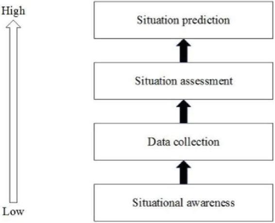
Figure 1 Conceptual model of network security situational awareness.
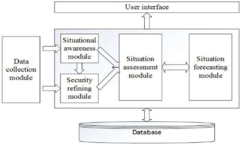
Figure 2 Network security situation awareness system framework.
(2) D-S evidence theory:
DS evidence theory is a fusion method that can solve the uncertainty of unknown problems. The Dempster synthesis formula is used to continuously fuse the trust functions of different evidences, and then gradually reduce the uncertainty of the problems as the evidence continues to accumulate. Thus, accurate inference results are obtained, and the decision logic can make corresponding judgments on the fusion trust function, and finally realize the evaluation [12]. D-S evidence theory often requires decision makers to generate a confidence distribution function based on the evidence they already have on the hypothesis space (or identification frame). This function can be used as the basic probability distribution function, or it can be called m function or mass function. By analyzing the evidence, the basic credible number m (A) of the proposition can be obtained, that is, the degree to which the proposition A is true.
For a decision problem, the set refers to all possible results that people can understand, so any proposition can be represented by a subset of the set . is therefore also called a frame of discernment (FOD). In other words, the frame of discernment represents the set of all possible results, and a proposition can be expressed as a set of possible results, which is equivalent to the knowledge base of propositions.
The observation of D-S evidence theory for the current system cannot uniquely determine some system states. A basic probability function (BPA) represents a function in which some evidence supports a system state. In other words, through the state probability function, we can calculate the probability of the system in a certain state according to some evidence.
Let be FDO, for the set function , if the formula (1) is satisfied:
| (1) |
Then is the BPA on the frame , where , is the basic credible number of . does not consider any of its true subsets and antecedents and consequences, but only responds to the trust of itself. Therefore, merely indicates the extent to which the evidence supports and not the true subset of . Mutual exclusion may occur in all possible sets of answers in the recognition frame .
Belief function, , that is, for arbitrary , as shown in formula (2):
| (2) |
The reliability function includes consideration of the cause and effect of each proposition, that is, if some evidence supports a proposition, it also supports the inference of the proposition. So the reliability of a proposition represents the sum of the evidence’s support for all its premises. The reliability function Bel can be understood as the total trust level of the subject for proposition , that is, the total support level.
If A represents a subset of and , then represents the focal element of the evidence, and the sum of all focal elements is expressed as the core.
Plausibility function: , for , as shown in formula (3):
| (3) |
refers to the likelihood of , which means that the degree of suspicion of is not doubted, or the maximum degree that can be trusted under the given evidence, and contains all the proposition sets compatible with A basic credibility. is more lenient than , and the relationship is as shown in formula (4):
| (4) |
Reliability functions and plausible functions support propositions in terms of pros and cons, respectively. usually indicates the uncertainty interval of a function, and refers to the degree of uncertainty of evidence.
The distribution of the above primitive focal elements indicates the degree of evidence’s support for the certainty of the true attributes of the proposition. The distribution of other non-primitive focal elements and represents the extent to which the evidence cannot fully determine the true attributes of the propositions or is completely unaware. The BPA of evidence refers to the degree of evidence support for focal elements.
The D-S synthesis rule says: Assuming , and are independent BPA on , as shown in Equation (5):
| (5) |
The size of reflects the degree of conflict of evidence. The larger the value of , the greater the conflict. represents the normalization factor, and its main function is to prevent the non-zero probability from being assigned to the empty set during the synthesis process.
If there are pieces of evidence to be synthesized, the synthesis rule is shown in formula (6):
| (6) |
If the evidences and are mutually supportive, and is the manifestation of the evidence-enhancing effect; if the evidences and are in conflict, then is canceled and suppressed. Shafer explained Dempster’s composition rule that both cases are more in line with people’s intuitive understanding of comprehensive evidence.
(3) Particle Swarm Optimization Algorithm:
Each particle in the particle swarm optimization algorithm is considered to be a potential solution to the problem to be solved. The calculation of the objective function adaptive value of all particles in the search space by the particles can make the particles continuously adjust the speed and position according to their own and other empirical knowledge until they reach the optimal. Particles can continuously adjust their position through their own flying experience and knowledge to achieve their best position (particle best, pbest); other particles’ flying experience and knowledge can make the current optimal position (global best, gbest) searched by the entire population Particles. Particle can update their speed and position according to formula (7) and formula (8):
| (7) | |
| (8) |
In the above formula, and represent the speed and position of particle through the -th iteration in the d-dimensional space; the coefficients and refer to the acceleration constant or learning factor. When the value is relatively small, it means Particles can be optimized within the target search area. When the value is large, the particles will rush towards or cross the target search area; and are random values between (0,1); w refers to the inertia weight, and has a very important influence on the algorithm [13], so that the particle swarm algorithm formula is more standard. When is small, it is conducive to local optimization and can improve the convergence speed of the algorithm; however, when is large, the algorithm can search for optimization in the global scope, which will help to jump out of local optimization; when , it means basic PSO algorithm. Particle swarm algorithm has fast convergence speed, easy to implement and relatively small parameters to be adjusted.
2.2 Prediction Related Theories
(1) Fuzzy C-means clustering
For the determined data set , the FCM algorithm can be used to divide it into c categories, where , and the cluster center of the -th category uses , to represent. In FCM, in order to indicate the degree to which a sample point is divided into a certain class by probability, a membership matrix is usually used. The membership matrix and optimization objective function are shown in Equation (9):
| (9) |
In the formula, refers to the distance between the sample and the cluster center , is the fuzzy index, , and is used to control the fuzzy degree of the membership matrix . When the size of is close to 1, the FCM degenerates into a hard C-means clustering. At this time, the degree of membership approaches 0 or 1. The value of is generally 2. But when increases, the corresponding ambiguity increases. When increases to infinity, the membership approaches 1/c.
Solve by Lagrange multiplication, as shown in Equations (10) and (11):
| (10) | ||
| (11) |
In the FCM calculation process, the relative calculation results cannot give a reasonable explanation if is relatively large, but if is relatively small, the classification will not be accurate enough. So the choice of is crucial to the result. The validity function can reasonably calculate the number of clusters [14]. Therefore, the final clustering number is determined according to the corresponding validity function.
(2) Genetic algorithm
The main characteristics of genetic algorithm are: the derivative and the function continuity are not continually limited during the operation of the algorithm, and the structure object can be directly operated; its global optimization ability is better and it has inherent implicit parallelism; a probabilistic approach is used in the optimization process, and in the process of searching for space, some definite rules can be automatically obtained and guided for optimization.
In the search process of genetic algorithm, it is not easy to fall into a local optimum, because genetic algorithm does not rely on gradient information; genetic algorithm is suitable for large-scale parallel distributed processing, and parallel search efficiency is quite high, because genetic algorithm is a global parallel random search method. It is easy to combine genetic algorithm with neural network, fuzzy theory and so on, which makes the performance of the algorithm better.
(3) Radial Basis Function Neural Network
Radial Basis Function Network (RBFNN) is a three-layer forward network based on the theory of function approximation. It simulates the neural network structure of the local adjustment and mutual coverage receiving domain in human brain, and has been approached by theorists according to the function approximation theory of radial basis function [15], which proves that if there are enough hidden node radial basis functions in the network, the RBF network can approach any continuous function.
RBF network consists of three layers: input layer, hidden layer and output layer. In this network, some input information can be transmitted through the input layer and then be transmitted to the hidden layer; the information in the input layer is processed mathematically and then transmitted to the output layer, which is mainly operated in the hidden layer, and there is a radial basis function in this layer; The output layer is mainly used as the output result after the weighted calculation of the hidden layer processing result is completed.
There are various forms of radial basis functions [16], but Gaussian functions are currently widely used. The input vector of the network can be represented by , and the network output vector can be represented by , usually represents the weight matrix from hidden layer to output layer, the corresponding hidden layer output is expressed as , refers to the output terms, each of which can be represented by a radial symmetric basis function The Gaussian function formula is shown in Equation (12):
| (12) |
The center and width of the Gaussian function are expressed by and , respectively. The number of nodes in the hidden layer can be expressed by .
The output is shown in Equation (13):
| (13) |
In this formula, refers to the connection weight of the -th output in the hidden layer and the -th neuron in the output layer, and represents the normalized output of the -th node in the hidden layer.
The radial basis function needs to learn three relatively main parameters: the basis function center, variance, and weight. There are relatively many choices for its center, and different centers correspond to different learning methods. At present, the most commonly used are: randomly selected center, self-organized selection center, supervised selection center method and orthogonal least squares method [17]. This article introduces the related self-organized selection method. The method mainly has two stages of organizational learning and supervised learning. For supervised learning, this method mainly performs corresponding operations on the weights of the corresponding output layers, while for organizational learning, this method can perform related operations on the radial basis functions. The learning center is temporarily represented by . In learning related operations, K-means (K-means clustering) algorithm can be used. We can temporarily assume that the number of cluster centers is I (the value is usually determined based on corresponding experience in the previous calculation process). Let refer to the center when the basis function iterates to the nth generation. The corresponding operation process is as follows:
1. First, determine the center of the cluster, select I different samples as the initial center by experience, and set the number of iteration steps n to 0;
2. Randomly input the sample ;
3. Find the closest clustering center of the sample , find , satisfy the following formula (14), represents the center of the -th basis function when adjusted to the -th generation:
| (14) |
4. Adjust the center by Equation (15):
| (15) |
5. For all samples, determine whether the corresponding operation has been completed and whether the layout remains the same. If the layout changes, then and go to step 2 to restart perform the corresponding input operation, otherwise end.
6. The thus obtained is the center of the basis function.
Because the center will not change after it is determined, the variance is determined next. If RBF selects Grauss, the function formula is shown in (16):
| (16) |
Among them, I represents the number of hidden layer neurons, and represents the maximum distance between the selected cluster centers.
represents the learning weight, which is mainly calculated using the least mean square (LMS) algorithm. The input signal in this algorithm represents the output of the RBF hidden layer. During the correlation output process, only the hidden layer neurons are weighted and summed. The formula is (17):
| (17) |
If the learning weights are calculated using a pseudo-inverse method, then:
| (18) |
In Formula 22, represents the expected response, ; are weight matrices, is the pseudo-inverse of matrix , , and , is calculated as Equation (19) shows:
| (19) |
3 Optimized Assessment and Prediction Methods
3.1 Improved Network Security Situation Assessment Model
This paper evaluates the network security from three levels: network layer, host layer and service layer. At the service level, the threat of each service is measured. In the host layer, the security threats faced by all services are superposed to form the host layer situation. In the system layer, according to the importance of each host, each host gives different weights, and synthesizes the host situation to get the situation value of the whole network security.
This paper proposes an improved network security situational awareness model, as shown in Figure 3.
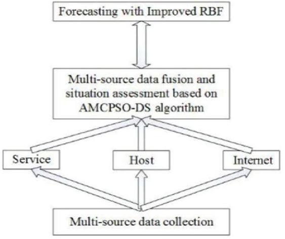
Figure 3 Improved network security situational awareness model.
In this model, information fusion is first performed on multi-source heterogeneous security data detected by multiple sensors, and the detected data is used for situation assessment. Subsequently, the situation assessment was conducted through three aspects of service, host and network, and the AMCPSO-DS algorithm was used to comprehensively assess the network security situation. In the process of network prediction, this paper uses an improved RBF neural network to predict the network security situation based on the safety data output from the situation assessment. The improved RBF neural network mainly uses the fuzzy C-clustering method to the number of neurons Determine it, then use the relay genetic algorithm to get the RBF neural network neuron center and width, and finally use the least squares method to calculate the hidden layer to the output layer weights, and finally use the improved RBF neural network to obtain a relatively accurate Situation predictions.
(1) Service security posture:
Within a period of time, the service has been subjected to different attacks . Because different attacks pose different threats to the service , so different attacks represent different levels, and can be used to represent the level. Some different attacks may also belong to the same level. The calculation of the threat factor of level is shown in formula (20):
| (20) |
By this formula, we can calculate the threat weight of different attacks to the service, which indicates the threat degree.
The quantified weights of different attack threat factors in are represented by , and the total number of different types of attacks suffered by service is represented by . The number of attacks of type is , and the security posture of the service is related to the degree of attack, as shown in Equation (21):
| (21) |
In the above formula, represents the security situation of service , represents the number of services, where is mainly used to determine the relevant threat the important role of factors.
(2) Host security posture
For a period of time, the service running by the host is represented by , and the importance of the service is expressed by according to the degree of adverse consequences for the host after the service fails. The security posture of the host is:
| (22) |
For the service in the host , the degree of threat is expressed by its importance, and then normalize it:
| (23) |
(2) Network security posture
The network security situation is composed of the host security situation and the number of hosts within a period of time. The network system NS has v hosts. The important weight of the host is , then the network system security posture is expressed as (24):
| (24) |
The importance of the host is mainly determined based on the number of relatively critical services on the host, the asset value, and whether there are more important data. You can use to represent, and then normalize it to get the host weight as:
| (25) |
3.2 Cross-layer Adaptive Mutation Particle Swarm Optimization
Introducing the mutation probability factor into the particle swarm position vector can enable the algorithm to effectively perform a global search and expand the search range of the solution space. However, if the mutation rate is too large, accurate local search cannot be performed on the population, and the efficiency will be reduced; if the mutation rate is too small, the population cannot escape the local extremum quickly and accurately. Therefore, the size of the variation factor must be adjusted according to the current environment, so as to enhance the adaptability of the variation [18]. By setting the threshold of the number of times the optimal position of the particle swarm is unchanged, the change of the optimal position of the particle swarm is judged. If the number of times that the best position of the particle group does not change is greater than the threshold, it means that the particles appear precocious.
If the particles appear premature phenomenon, the position vector of particle swarm is randomly mutated by mutation factor. At each iteration, the judgment starts after the particles update the velocity and position vectors. The variation formula of particle position vectors is shown in 26, where is the mutation operator, is the random number between (0,1), and C is the variation factor [19]:
| (26) |
In this paper, a cross-layer particle swarm optimization with adaptive mutation (AMCPSO) was studied to improve this problem, as shown in Figure 4.
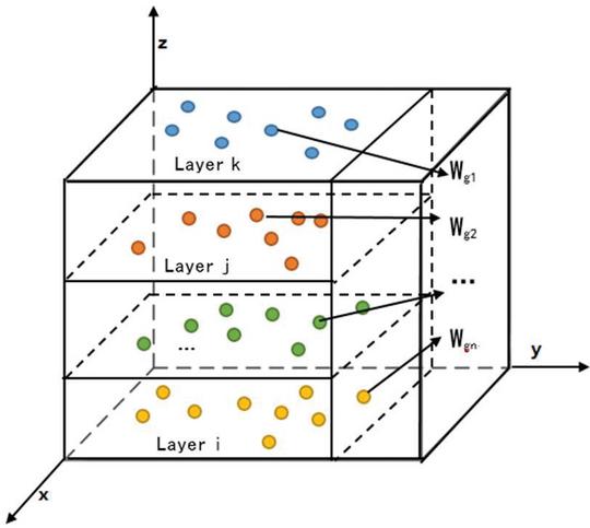
Figure 4 Cross-layer adaptive mutation particle swarm optimization.
The speed and position are continuously updated according to AMCPSO, and the weights of the D-S evidence fusion process are optimized. The updates are shown in formulas (27) and (28):
| (27) | |
| (28) |
Where , refers to the number of particles that need to be correlated, , are constants, will take any value from [0,1]; w is the decreasing inertia Weight. Related parameters often need to be restricted by related functions when performing a series of fusions and finding the best value, as shown in Equation (29):
| (29) |
This formula is a fitness function, and refers to the fitness function of . In this formula, represents the number of propositions, refers to BPA, and represents the BPA value of that needs to be decided. The category of the decision target is mainly based on the difference between the decision target BPA and other non-decision target BPAs after weighted fusion. Therefore, under the constraints of the fitness function, AMCPSO can determine different exponential fusion weights for sensors containing different data sources: . So the information fusion is shown in formula (30):
| (30) |
3.3 Improved RBF Neural Network
This paper uses the FCM method and the validity function to calculate the number of neurons in the first stage. In the second stage, the genetic algorithm is used to determine the center and extension width. Then, the output weights are calculated by the least square method.
Hierarchy Genetic Algorithm (HGA) is a method that uses a combination of binary and real number coding, and belongs to a hybrid method. During the operation of the algorithm, the parameters and structure of the neural network can be optimized, so the algorithm has better efficiency.
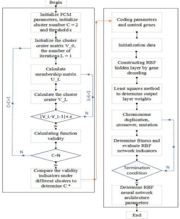
Figure 5 Improved HHGA-RBFNN flowchart.
The improved RBF neural network learning algorithm based on hybrid hierarchical genetic algorithm (HHGA) is shown in Figure 5:
1. Determining the number of neurons: First, determine the number of neurons, that is, use FCM clustering method and effectiveness function to comprehensively evaluate, and finally determine the optimal result is the number of neurons.
2. Initialize the network: Determine the population size as , and choosing the exact population number is of great significance to the convergence of the algorithm. According to experience, is generally set to 20–160. During training, the maximum value of the control gene is set to , so the number of hidden layer nodes is . The size of the parameter gene initialization is a random value between [0, 1].
3. Fitness function: it is hoped that the value of the comprehensive index can be trained to the lowest value, that is, it has a simple network structure under a certain accuracy requirement. The precision objective function is shown in Equation (31):
| (31) |
In this formula, refers to the real output value of the network, and refers to the desired output value. The calculation result of the entire formula represents the error between the actual and the desired output.
In order to control the structure and accuracy of the network, the fitness function takes the following form:
| (32) |
In this formula, is the number of samples, is the number of hidden layer nodes, is the expected output value, is the actual output value of RBFNN, and is an arbitrarily large value that can be reached. This formula represents the fitness function of the minimum information criterion (AIC), and this article will use this function as the objective function.
4. Genetic operation: This operation process is mainly for some chromosomes with the highest fitness value. If the fitness of an individual is greater, the probability of this individual being selected will be relatively greater. These chromosomes are selected for subsequent selection and replication operations.
The expected value of the individual is calculated using the expected value method:
| (33) |
In this formula, represents the fitness of individual i, refers to the average fitness, represents the overall fitness of the population, and represents the population size.
The expected value of the individual determines whether the corresponding individual in the population can enter the next generation. The population changes from P1 to P2 through selection and replication operations, followed by crossover and mutation operations. The role of crossover is to generate new gene combinations to form population P3. Because parameter genes and control genes are encoded differently, crossover operations need to be performed separately. The control gene cross follows the rules of binary coding, that is, a one-point cross operation.
Because the parametric genes are encoded in real numbers, they need to mimic the corresponding operations. Perform the corresponding operation according to formula (34):
| (34) |
In this formula, a is a random number of , and and are from the parent and are arbitrarily selected.
Through the mutation operation, the number of individuals in the population will increase, thereby ensuring that the search is performed in a relatively large space. The mutation operation randomly selects an individual from the population P3 based on the mutation probability, and forms a population P4 by randomly changing one or some genetic loci in the individual.
The crossover rate and mutation rate are usually adaptively selected. The crossover probability and mutation probability are calculated according to (35) and (36):
| (35) | ||
| (36) |
In the above formula, represents the maximum fitness of the current population, refers to the average fitness of the population, ‘indicates that the individual fitness among the parents to be crossed is relatively large, and f is the fitness of the mutated individual. are all in the range of (0,1), given , .
It can be concluded that and will increase when the fitness of each individual in the population is consistent or locally optimal, but and will decrease when the fitness of the population is relatively scattered.
4 Simulation Experiments
This article uses the network topology shown in Figure 6, and uses Netflow, Snort, and Snmap to detect data at each layer. The opened services include WWW, FTP, DNS, HTTP, RPC, and TELNET.

Figure 6 Experimental environment.
The data set in this paper is selected from the DARPA 99 data set published by Wenke Lee and others in the 1998 Department of Defense Advanced Research Project. The data set contains about 5,000,000 pieces of data, including seven weeks of training data, and about 2,000,000 pieces The test data mainly includes four types of attacks, Probe, U2R, DOS, and R2L. This article selects a part of the data from it.
4.1 Evaluation Simulation
This paper aims at the DARPA data set and fuses multi-source data according to related topologies and algorithms, and evaluates the network security situation accordingly. The experimental process is carried out using MATLAB7.0 toolkit.
In order to make the experimental data have the same proportion of attacks as the original data set, this article samples the experimental data and extracts each type of data according to the proportion of the original data. Table 1 shows the distribution of selected training data, and Table 2 shows the distribution of selected test data.
Table 1 Training data set
| Attack Category | Dos | probe | U2R | R2L | Normal |
| Number of attack instances | 97084 | 1027 | 32 | 232 | 24319 |
Table 2 Testing data set
| Attack Category | Dos | Probe | U2R | R2L | Normal |
| Number of attack instances | 41607 | 440 | 13 | 99 | 10422 |
Netpoke is used to replay the data set to ensure that the network conditions of the system can simulate the real network conditions to the maximum extent. XML technology is used to transfer and format cross-layer heterogeneous sensor data. The detection results of the three types of sensors, Netflow, Snort, and Snmap, are used for the multiple fusion training using the AMCPSO-DS algorithm. The population size is set to 50, and the weights are optimized in the range . Because noise often has a certain impact on the weight in the actual operation process, this paper combines offline optimization and online adjustment to reduce the impact on the optimization weight. For the heterogeneous sensor BPA, the expected deviation, the rate of change of the Netflow port, and the flow in / out ratio can be used for corresponding acquisition. Table 3 shows the calculation results of the corresponding BPA and weights.
Table 3 Weights and BPA
| Attack Category | Dos | probe | U2R | R2L | Normal |
| Netflow(BPA) | 0.279 | 0.364 | 0.142 | 0.098 | 0.109 |
| snort(BPA) | 0.183 | 0.286 | 0.200 | 0.190 | 0.129 |
| Snmp(BPA) | 0.162 | 0.189 | 0.260 | 0.346 | 0.031 |
| Netflow(w) | 0.92 | 0.88 | 0.21 | 0.25 | 0.52 |
| snort(w) | 0.35 | 0.61 | 0.89 | 0.69 | 0.63 |
| Snmp(w) | 0.24 | 0.39 | 0.70 | 0.66 | 0.31 |
| Threat level | 2 | 3 | 1 | 1 | 0 |
By replaying the test data set, this article compares AMCPSO-DS with traditional D-S, PSO-DS, and CPSO-DS in terms of detection rate (TDR) and false positive rate (FOR). The results are shown in Table 4.
Table 4 Performance comparison
| Parameter | TDR | FDR |
| Traditional D-S(%) | 73.82 | 9.91 |
| PSO-DS(%) | 86.61 | 5.52 |
| CPSO-DS(%) | 88.10 | 5.07 |
| AMCPSO-DS(%) | 89.32 | 4.99 |
The experimental results show that the method proposed in this paper improves the attack detection rate and false positive rate.
The perception of network security situation usually requires the determination of the importance weight of the host, host weight and host asset value , service criticality , access frequency level , and confidentiality And other factors. The compound importance of the host , , , ?
For the situation calculation, this experiment takes days as the time unit, and according to the previous calculation method in each time unit, the experiment is tested and evaluated for 10 weeks. The daily data is processed and quantitatively calculated to obtain the corresponding evaluation value. However, since the calculated original situation value is large, the situation value is normalized. The experimental results are shown in Figure 7.
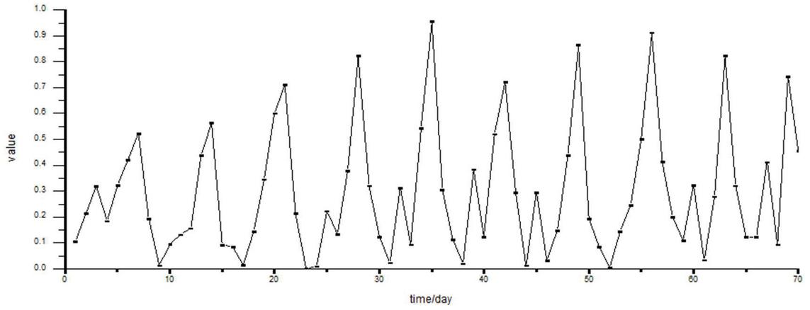
Figure 7 Network security situation.
From the experimental results, it can be seen that the network security situation assessment method proposed in this paper is close to the actual situation value, and has achieved good results.
4.2 Predictive Simulation
According to the network security data provided and the trained RBF neural network, the obtained historical value and current situation values are used to predict the network security situation. Because the situation assessment experiment has always obtained seven weeks of data, the situation of the next week is predicted from the data of the first six weeks, as shown in Table 5 and Figure 8.
Table 5 Forecast results
| The First Week | The Second Week | The Third Week | The Fourth Week | Fifth Week | Sixth Week | Seventh Week | |
| Actual | 0.3212 | 0.1232 | 0.1234 | 0.4122 | 0.0932 | 0.7432 | 0.4561 |
| Forecast | 0.2871 | 0.1089 | 0.1993 | 0.3598 | 0.1232 | 0.7519 | 0.1989 |
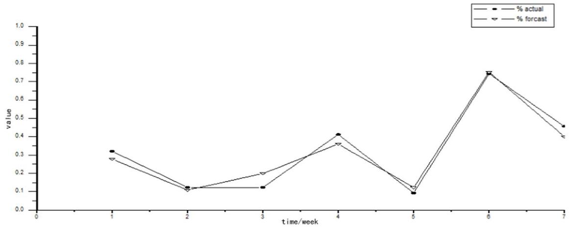
Figure 8 Situation prediction.
In Figure 8, the rectangular curve represents the actual situation value, and the triangular curve represents the prediction value of network security situation according to the improved RBFNN algorithm, so it can be seen that the prediction result is close to the actual result, so the method has a better prediction effect.
5 Conclusion
The AMCPSO-DS algorithm proposed in this paper has better advantages than traditional algorithms in multi-source data fusion, and can effectively integrate more comprehensive network security information to evaluate the security status of the network; the prediction effect of the improved RBF neural network on network security situation is compared with the actual value Close, thus proving the feasibility of the method. The algorithm proposed in this paper has certain reference significance for the research work related to network security situational awareness.
In the next step, we will study the following work:
1. This paper lacks the research on situation visualization. The visualization is mainly based on the situation assessment and prediction results to dynamically present to the network administrator to better manage the network environment. Therefore, we will focus on this aspect in the future.
2. The research on network security situation in this paper is only a simulation experiment based on DARPA data set, and lacks the research on the actual network environment. Therefore, the next step is to study the network security situation in the real network environment.
Acknowledgements
The authors acknowledge the National Natural Science Foundation of China (Grant: 61672206), The Key Research and Development Program of Hebei (No. 20310701D).
References
[1] Kodagoda, Neesha (2014). Concern level assessment: Building domain knowledge into a visual system to support network-security situation awareness. Information Visualization, 13(4), 346–360.
[2] Tim Bass (2000). Intrusion Detection Systems and Multisensor Data Fusion: Creating Cyberspace Situational Awareness. Communications of the Association for Computing Machinery. 43(4), 99–99.
[3] Lau S (2004). The spinning cube of potential doom. Communication of the ACM, 47(6), 25–26.
[4] Maleh Y, Ezzati A (2015). Lightweight Intrusion Detection Scheme for Wireless Sensor Networks. IAENG International Journal of Computer Science, 42(4), 347–354.
[5] Zhu L N, Xia G N, et al. (2016). Multi-dimensional Network Security Situation Assessment. International Journal of Security & Its Applications, 10(11), 153–164.
[6] Moosavi H, Bui F M (2017). A Game-Theoretic Framework for Robust Optimal Intrusion Detection in Wireless Sensor Networks. IEEE Transactions on Information Forensics and Security, 9(9), 1367–1379.
[7] Shi Y Q, Li R F, Zhang Y, et al. (2015). An immunity-based time series prediction approach and its application for network security situation. Intelligent Service Robotics, 8(1), 1–22.
[8] Chen S X, Yang Zh, Zhu J, et al. (2015). Network security situation prediction method based on PSO-SVM. Application Research of Computers, 32(6), 1778–1781.
[9] Li F W, Zhang X Y, Zhu J, et al. (2016). Network security situation prediction based on APDE-RBF neural network. Systems Engineering and Electronics, 38(12), 2869–2875.
[10] Beng L Y, Manickam S (2016). A Novel Adaptive Grey Verhulst Model for Network Security Situation Prediction. International Journal of Advanced Computer Science & Applications, 7(1), 90–95.
[11] Shi Y Q, Li R F, Peng X N, et al. (2016). Network Security Situation Prediction Approach Based on Clonal Selection and SCGM(1,1)c Model. Journal of Internet Technology, 17(3), 421–429.
[12] Zhao G Z, Chen A G, Lu G X, et al. (2020). Data Fusion Algorithm Based on Fuzzy Sets and D-S Theory of Evidence. Tsinghua Science and Technology, (1), 12–19.
[13] Wang L, Dong C H, Hu J P, et al. (2015). Network Intrusion Detection Using Support Vector Machine Based on Particle Swarm Optimization. Plant Biotechnology Reports, 4(3), 237–242.
[14] Yan X H (2015). Mining Network Security Logs via Fuzzy Clustering Algorithm. Journal of Computational & Theoretical Nanoscience, 12(12), 6220–6226.
[15] Li X, et al. (1998). On Simultaneous Approximation by Radial Basis Function Neural Networks. Applied Mathematics and Computation, 95(1), 75–89.
[16] Han H G, Lu W, Hou Y, et al. (2016). An Adaptive-PSO-Based Self-Organizing RBF Neural Network. IEEE Transactions on Neural Networks and Learning Systems, (99), 1–14.
[17] Zhu W X (2016). Network Intrusion Prediction Model based on RBF Features Classification. International Journal of Security & Its Applications, 10(4), 241–248.
[18] Ji W D, Sun L P, Wang K Q, et al. (2016). An Improved Particle Swarm Optimization Algorithm of Radial Basis Neural Network. International Journal of Control & Automation, 9(10), 413–420.
[19] P Asokan, J Jerald, S Arunachalam, et al. (2008). Application of Adaptive Genetic Algorithm and Particle Swarm Optimisation in scheduling of jobs and AS/RS in FMS. International Journal of Manufacturing Research, 3(4), 393–405.
[20] Wang H Z, Ruan J Q, Ma Z W, Zhou B, Fu X Q, et al. (2019). Deep learning aided interval state prediction for improving cyber security in energy internet. Energy, 174(174).
[21] Pu Z Y (2020). Network security situation analysis based on a dynamic Bayesian network and phase space reconstruction. Journal of supercomputing, 76(2), 1342–1357.
[22] Shen H J, Wan W, Long C, et al. (2019). Security Situation Assessment Method Based on States Transition*. 2018 IEEE International Conference on Information and Automation (ICIA). IEEE.
Biographies

Dongmei Zhao, Doctor of Engineering (Master of Network Security), Professor. Graduated from the Xidian University in 2007. Worked in Hebei normal university. Her research interests include network security situation estimation and prediction.

Hongbin Wang, studying in Computer Science and Technology, College of Computer and Cyber Security, Hebei Normal University. His research interests is network security.

Xixi Li, master of applied software technology, graduated from Hebei Normal University in 2018. Her research interests include network security situation estimation and prediction.
Journal of Web Engineering, Vol. 19_7-8, 1239–1266.
doi: 10.13052/jwe1540-9589.197814
© 2020 River Publishers