Improved IDR Response System for Sensor Network
A. Kathirvel*, M. Subramaniam, S. Navaneethan and C. Sabarinath
Department of CSE, Faculty of Engineering and Technology, SRM Institute of Science and Technology, Vadapalani, Chennai, Tamilnadu, India
E-mail: kathirva@srmist.edu.in; subramam2@srmist.edu.in; ns2066@srmist.edu.in; sabarinc@srmist.edu.in
*Corresponding Author
Received 09 September 2020; Accepted 31 October 2020; Publication 15 February 2021
Abstract
Wireless sensor network (WSN) is highly sophisticated than ad hoc wireless network. Ad hoc wireless network is mostly affected by different resources such as high processing energy, storage capabilities and battery backup and etc. Due to the open nature, poor infrastructure, quick deployment practices, and the conflict environments, make them susceptible to a wide range of attacks. Recently, the network attack affects the performance of networks such as network lifetime, throughput, delay, energy consumption, and packet loss. The conventional security mechanisms like intrusion detection system (IDS) of network security are not enough for these networks. In this thesis, we introduce an enhanced intrusion detection and response (EIDR) system using two tire processes. The first contribution of proposed EIDR system is optimal cluster formation and performed by the chaotic ant optimization (CAO) algorithm. The second contribution is to calculate the trust value of each sensor node using the multi objective differential evolution (MODE) algorithm. The computed trust value is used to design the intrusion response action (IRA) system, which offers additional functions and exhibit multiple characteristics of response to mitigate intrusion impacts. The simulation results display that the proposed EIDR system has a better detection rate and false positive rate without affecting network performance.
Keywords: WSN, EIDR, CAO, MODE, IRA, and IDS.
1 Introduction
WSNs are distributed volatile sensors to monitor the physical or environmental conditions like temperature, pressure, sound and synchronize their data with the network. Due to the continued development of wireless sensor networks, the need for more effective security mechanisms is also increasing. The security issues of the sensor network should be addressed by the beginning of the design of the system because the sensor networks interact with sensitive data and generally work in hostile unpredictable environments. Wireless Sensor Network requires a detailed understanding of the capabilities and limitations of each basic technology for secure work. At each end of the WSN, the design should be designed to provide the main sources of synchronization of the combined topology package, which is strict energy consumption. The protection of the connection to the group that requires the delivery of packages from one or more of the senders is a major objective Bleda et al. (2017), Wu et al. (2016), and Jokhio et al. (2013).
An intrusion detection system (IDS) attempts to detect Valeur et al. (2004) insecure conditions of networks due to the malicious attacks. Intrusion is a set of events that can lead to unofficial access or change of wireless networking system. IDS methods can detect cruel intruders from those anomalies and to monitor the system’s behavior, to identify the existing intrusions in the network, and to alert the users after the intrusion has been identified, to re-enter the network if this is possible Mishra et al. (2004). Generally, the neighbors of a malicious node are the first to learn those abnormal behaviors. Therefore, it is easy to let every node control its neighbors in such a way that the IDS mechanism can be activated as soon as possible Ye et al. (2004). IDS observe and analyze the maximum security problems in the network system, track unusual events and it is used to monitor the network. The principal approaches for IDS are classified into two: misuse detection and anomaly detection. Misuse detection technique compares the behavior observed with known attack signatures. Action patterns that cause security threats should be defined and stored in the system. The advantage of this technique is that it can detect instances of known attacks accurately and efficiently, But it does not have the ability to detect unknown type of attack Ye et al. (2004). Anomaly detection Erbacher et al. (2002) is based on the general behavior of a system and it compares normal activities against the events observed for identifying important deviations.
In recent years, many IDS are proposed for WSN. IDS employed as a second line of defense are mandatory to provide a high security information system and it can effectively identify intruders and thus provides intensive security Hoyle et al. (2015). The intrusion detection models are single-sensing detection and multi-sensing identification used to detect intrusion in both homogeneous and heterogeneous WSN by showing the probability of intrusion detection with distance and network parameters Sun et al. (2007).
An enhanced intrusion detection and response (EIDR) system is proposed using two tier processes are optimal clustering and trust computation. The IDS module classifies the type of malicious present in the network and the IRS module is responsible to make the response action of particular malicious problem in data transmission path. The main objective is to maximize the detection rate and minimize false positive rate without affecting the network performance such as network lifetime, throughput, end-to-end delay, energy consumption, and packet loss.
The remainder of the paper is organized as follows. Above Section briefly reviews the recent papers related to our contributions. In Section 2, problem methodology of IDS system and system model of proposed solution is presented. The brief discussion of proposed EIDR system is given in Section 3 with proper mathematical models. The simulation results are analyzed in Section 4. Finally, the paper concludes in Section 5.
2 Problem Methodology and Network Model
2.1 Problem Methodology
Security is a key issue for each and every one of the structures of affiliation and foundations at the present time and each and every one of the checks are attempting in ways that actuating access to the data design of these affiliations. IDS is an inside and out new advancement of the structures for dangerous unmistakable assertion procedures that have made starting late. The run some bit of IDS is to help PC structures with planning and deal with the framework ambushes. Interference ask for limits wires checking and executing both customer and structure works out, withdrawing system setups and vulnerabilities, looking over structure and record unfaltering quality, ability to see plans ordinary of ambushes, examination of atypical change cases and following customer procedure encroachment. The goal of impedance zone is to screen manage focal obsessions for see sporadic lead and abuse in regulate. Jin et al. (2017) have proposed IDS using a multi-agent system and a node trust value (MTID). The multi-official display structure is made in both the bundle heads and standard sensor centers to perform impediment unmistakable proof. Customary obsession point trust properties are delineated and pull back hypothesis is used to judge whether these characteristics are standard.
Starting late, by far most of the IDS are secured to arranging layer essentially, regardless it can be moved to see aggregated sorts of strikes at different structures association layers as well Bleda et al. (2017), Wu et al. (2016), Jokhio et al. (2013), Valeur et al. (2004), Mishra et al. (2004), Ye et al. (2004), Erbacher et al. (2002), Hoyle et al. (2015), Sun et al. (2007), Yun Wang et al. (2008), Shin et al. (2010), Bu et al. (2011), Bao et al. (2012), Wei and Kim (2013), Chen et al. (2013), Abduvaliyev et al. (2013), Sun et al. (2013), Matyas and Kur (2013),Moosavi and Bui (2014) and Han et al. (2013). Two or three sees just interference and some achieve more like getting more information e.g. sort of ambushes, regions of the gatecrasher et cetera. Regardless of the way that a partner with number of IDS instruments are used yet not an enormous measure of them can be fitting for WSN with their slant slants Deif and Gadallah (2017). From existing works Han et al. (2014), Lin et al. (2016), Pintea et al. (2015), Huang et al. (2017), Zhang et al., 2017, Mrugala et al. (2017), Sedjelmaci et al. (2017), Guo et al. (2017), Santoro et al. (2017), Alsaedi et al. (2017), Jin et al. (2017), IDS are not speaking to shield WSN from Inside and Outside aggressors. None of them are done case most by a wide edge of the strategies offer social affair frameworks without picking how they will be kept and by what procedure will they continue with rest of the structure. In context of their open nature and nonattendance of structure, security for WSNs has changed into a confounding issue than the security in various frameworks. The standard security frameworks of guaranteeing wired structure are not appealing for these structures. Thus, proposed EIDR system overcome those problems by two tire process such as clustering and trust evolution. The main contribution of proposed EIDR system is summarized as follows:
1. In EIDR system, the chaotic ant optimization (CAO) algorithm is used to form the cluster using the sensor node constraints such as position and velocity, which provides stable and energy efficient clusters.
2. The multi objective differential evolution (MODE) algorithm is used to compute the trust of each sensor node, which used to make routing between source-destination with the help of basic low-energy adaptive clustering hierarchy (LEACH) protocol. Then, perform IRA using the computed trust value with the actions are no punishment (NP), punishment (P) and isolation (I).
3. The proposed EIDR system is tested with high density nodes in network simulator (NS-2) with three different network attacks are selective forwarding, denial of service (DoS) and flooding attacks.
2.2 Network Model
In EIDR system, we assume network consists of randomly distributed high density nodes and malicious nodes without movement. The sensors present in the network have same transmission range and unique ID for user identification. The routing pattern is followed by the basic LEACH protocol with the help of our computed trust values. That is to say, the sensed information’s from each sensor are forward to next node that is selected by trust value.

Figure 1 EIDR systems with example trust values and attacks.
The routing implies that nodes only directly communicate with their highest trust neighbor nodes. Also, the information’s forwarded between neighbor nodes are depends on the trust value, which cannot only transfer the packets from source nodes to destination nodes, but also process the packets based on specific requirements. The assumed network model of proposed EIDR system is shown in Figure 1 with example trust values and attacks.
3 Enhanced Intrusion Detection and Response System
The IDS used to detect the attacks. Even if the system cannot prevent the attacks from getting into the network, noticing the intrusion will provide the security officer with valuable information. The detailed description of proposed Enhanced Intrusion Detection and Response (EIDR) system is present in the following section. EIDR consists of two algorithms namely clustering using CAO (Chaotic Ant Optimization) algorithm and Trust computation using MODE (Multi Objective Differential Evolution) algorithm.
3.1 Clustering Using Chaotic ant Optimization (CAO) Algorithm
Deif and Gadallah (2017) proposed Ant colony optimization (ACO) is a metaheuristic figuring for combinatorial change issues. The key idea of ACO figuring is the mix of from the earlier data about the structure of a promising plan with a posteriori data about the structure of formally got staggering systems. Metaheuristic estimation are checks which, with a specific common made obsession to escape from neighborhood optima, drive some enormous heuristic: either a central heuristic begin from an invalid method and adding bits to store up an OK entire one, or a near to ask for heuristic begin from a total approach and iteratively changing some of its parts to accomplish a typical one. The metaheuristic part interfaces with the low-level heuristic to secure plans superior to anything those it could have accomplished alone, paying little regard to whether iterated. The controlling piece is pro either by influencing or by randomizing the philosophy of close neighbor answers for considers in neighborhood look or by joining parts taken by various structures. The standard key thought, everything considered began by the lead of veritable ants, is that of a parallel range for after in excess of a not a lot of computational strings in setting of neighborhood issue information and on a dynamic memory structure containing data on the probability of early got result. The aggregate direct moving out of the relationship of the specific demand strings has shown standard in controlling combinatorial streamlining issues.
Here, the central ACO computation is invigorated by chaotic manner i.e. chaotic ant optimization (CAO) count to make best faultless squeezing. Exactly when ants see assistance, they attempt to keep up a proportionate edge with the light to fly in straight line. Here, the game-plan of ants is tended to in a structure. For each and every one of the ants, there is a get-together to secure the looking regards. The second parts in the estimation are foods tended to in a structure F, and a social gathering for securing the looking regards. The CAO algorithm starts with the initialization process, which approximates the global optimal of the optimization problems and defined as follows:
| (1) |
Where represents the function of random population , represents the moth’s movement around search space , represents the termination criteria . After the instatement, function is iteratively keeping running until the point that the minute that the cutoff returns outstanding kept. For the refinement in reflecting the direct of ants, the condition of every underground offensive irrelevant creature restored concerning sustenance as takes after:
| (2) |
Where represents the spiral function, and represents the i-th moth, j-th food respectively. Spiral’s initial point should begin from the underground bug and end at the last point ought to be the condition of the sustenance. Change of the level of winding pound the intrigue space. A logarithmic spiral is defined for the CAO algorithm as follows:
| (3) |
Where indicates the distance of the -th ant for the -th food, represents the shape of the logarithmic spiral, and random number respectively. From this condition, the running with position of an underground bug is portrayed concerning a help. The parameter in the winding condition depicts how much the running with position of the moth ought to be near the sustenance. With a specific extraordinary obsession to collect the sensible approach of individuals against troublesome joining and enable the mixing speed, we enhance the CAO check by the Levy-flight. It has the unmistakable properties to cover away the not dazzling get-together of masses, innovatively, which can make this appropriately ricochet out of the zone wrap up. The new position of ants is updated as follows:
| (4) |
Where is a random parameter which conforms to a uniform distribution, is take as 1, 0, and . Levy-flights are a kind of random walk in which the steps are determined by the step lengths, and the jumps conform to a Levy distribution as follows.
| (5) |
Where represents the standard normal distributions, , represents the standard Gamma function. To show up, global search cutoff of this figuring upheld utilizing remarkable stroll around Levy-flight, it is being gotten in neighborhood smallest is adjusted, and it to the degree anyone knows gives more triumphs especially to strike and multimodal benchmark limits. The planning improvement of proposed CAO estimation is given in Algorithm-1.
Algorithm 1 Cluster formation using CAO algorithm
1: Input: X population size, F number of design variables, termination criterion
2: Output: cluster formation
3: Initialize the position and distance of populations.
4: Compute initial solution using Equation (3), and identify best and worst solution in the population.
5: Modify the population solution using Equation (4).
6: Update the new solution if is better than old, otherwise maintain old one.
7: Stop the process if termination reached.
8: Return: Cluster formation
3.2 Trust Computation Using Multi Objective Differential Evolution (MODE) Algorithm
Differential evolution (DE) algorithm [33] is branch of transformative program for reestablish issues over pleasing spaces. The upsides of DE are its sensible structure, solace, speed and power. DE is striking harm from other fundamental effect suggests coordinating issues with the colossal encircled to respected domains. DE is a procedure contraption of gigantic utility that is in an inconsequential minute open for satisfying applications. DE has been utilized as a touch of two or three science and building applications to find influencing reactions for sensibly unmanageable issues without join as one with star information or complex strategy estimations. In the event that a structure is obliging to being continually analyzed, DE can give the best way to deal with oversee manage sort out expelling the best execution from it. DE utilizes change as a demand structure and choice to amass the power toward oversaw regions in the possible locale. Here, to vivify the consistent DE figuring by multi-objective DE (MODE) estimation utilizing the moving focuses, for example, criticalness utilize, got hail quality, administer lifetime and stop up rate. The detailed description of each constraint as follows.
3.2.1 Energy model
The way that most energy models considered are made in light of estimations made on utilitarian liberal fixations, and these models change just to the parts used as a touch of the executed contraption setup and working rely on that kind of focuses, these models are not traditionalist, and can be used only for reenactment and evaluation of sensor pack for which they were made. For WSN applications are to an inconceivable degree collected, and possible applications are unending, so it is crucial to execute a general enormity appear, nonexclusive and all the more little. The monstrosity use amidst conditions of rest and dynamic states can be intervened after some time. For a node to operate autonomously sense the average energy scavenged must be greater than or equal to the energy consumed by the node. The average energy consumption defined as follows:
| (6) |
Where is the power consumed by the node in its active state during and is the rate of occurrence, and that is the power consumed by the node in its inactive state and has the occurrence rate and lasts for a period equal to . Given the diversity of energy collection methods, and the wide range of application profiles it is not possible to create a generic model, however, the essential criterion is that the energy stored in the node must be at least equal with the energy used for its operation in the time interval .
| (7) |
Where the power is consumed by the sensory node in the time interval and is the power collected and stored power in the same timeline. General working of sensor bases expected a particular power supply, which for the periods in which handset and sensor are not utilized, when they are either wrapped up by electronic switches, or set into rest state, it is in a perfect world to be set to affect a lower to yield voltage through part vapor sorption system in light of the way that the criticalness sound judgment of the microcontroller will increment amidst these seasons of rest states. The total energy consumed by sensor node will be represented as follows:
| (8) |
Where , , , and is the energy consumption due to control unit, communication unit, sensor unit, and DC-DC converter respectively.
3.2.2 Received signal strength
The received signal strength represents the most major and the basic metric to assess the bit between the sensor living spaces for the restriction objectives. In the got flag quality based block structures, the signal strength received at the sensor focus point is mapped into divisions by systems for certain channel show up. The received power at the sensor nodes employing the log normal shadowing model is represented as follows:
| (9) |
The mathematical equation for the path loss function evaluated and expressed in decibel is represented as follows:
| (10) |
Where is the distance between sending and receiving nodes, denotes the near earth reference distance corresponds to the path loss index signifies the zero-mean Gaussian random noise. The path loss function represented in terms of the transmitter and receiver is furnished by as follows:
| (11) |
Where and denotes the transmitted and receiver signal power respectively. The value of path loss index is invariably dependent on the environment or the transmission scenario. The distance is considered as one meter for the sake of easy evaluation. The basic edition of Equation (10) may be expressed with respect to the received power as follows:
| (12) |
3.2.3 Network lifetime
The network lifetime (NL) is the weighted whole of whatever is left of the lifetime of individual sensors of the baffling number of sensors in the sensor plot. The straggling stays of the lifetime of individual sensor is depicted as the made holding up criticalness out of the sensor at minute. In the preparing of the sensor manage, the centrality is depleted when the sensor gets or passes on something specific. By uprightness of the wobbly remote correspondence in WSN, the bundle might be retransmitted to ensure the right transport. The criticalness of each inside and their condition in like way used to pick remaining lifetime of the entire sensor make. We consider the straggling bits of the lifetime of the entire sensor regulate as the aggregate of the weighted extra lifetime of all sensors in the sensor network. Thus, the remaining lifetime of the whole sensor network (NL) as follows:
| (13) |
Where represents the weight factor of each sensor node counts. Weight factor is the nearer the sensor to the CH, the more important it is. The weight of each sensor represented by,
| (14) |
Where represents the constant. The weighted sum of remaining lifetime of individual sensors computed as follows:
| (15) |
3.2.4 Congestion rate
The congestion rate (CR) is utilized to study the store of sensor focus. Every wide enchanting fixation can adaptively watch the event of cripple and a short cross later impact the parent focuses to reduce the bundle transport rate as appeared by the blockage level. The bare rate of each node is calculated as follows:
| (16) |
Where the bare rate of the node is and ; is the node importance index, which computes a quantitative indicator. It can be defined as,
| (17) |
Where represents the connectivity degree describes how close the node is to neighbors. A coverage probability to represent the connectivity degree and obtained as,
| (18) |
Where represents the edge number from to on node .
MODE depends on individuals and goes for overhauling general multi-specific motivations driving limitation. It utilizes the change manager as to give the trading of data among a few blueprints. It utilizes three developmental parameters and significant errands, for example, increment, subtraction, examination, and its execution is proportionate or even beats other transformative or heuristic estimations. The immediate purpose of joining of MODE is to registers the general immaculate of a most pivotal over eager space. In particular, and without loss of generality, this problem can be reduced to finding the minimum of a function:
| (19) |
Where is dimensional vector and is a real function of real-valued arguments.
Differential evolution algorithm requires just three parameters, for example, mutt and change sharpens that are everything seen as continued, scaling some piece of the refinement of two people and masses size to make the developmental technique for D-dimensional issue. The check begins with introduction process considering parameter respects that are particularly scattered between the pre-shown disengage down beginning parameter bound and the upper initial parameter bound as follows:
| (20) |
In order to generate a trial vector, first changes the objective vector , from the present individuals by including the scaled multifaceted nature of two vectors from the present masses with the mutant vector . Records and are subjectively picked with the condition that they are surprising and have no relationship with the iota report by any structures (i.e. ). The change scale factor is a positive superior to normal encompassed number, however a mind blowing bit of the time as could sensibly be common short of what one. The process of mutant vector generation is given as follows:
| (21) |
In order to increase the diversity of the parameter vector, the crossover operation is applied to the mutant vector and the original individuals . The result is a trial vector , which is computed as follows:
| (22) |
The crossover parameter controls the bit of parameters that the mutant vector is adding to the last trial vector. In like way, the trial vector dependably gets the mutant vector parameter as appeared by the subjectively picked record. This MODE check is utilized to figure the trust in estimation of each inside point. Here, our devotion is to pick require level of each inside; the standard DE [33] performs just with two-dimensional factors yet MODE tally handle D-dimensional vectors and it can particularly sensible to figure confide in an enlivening power as important and perfect way.
4 Simulation Experiments
We use a simulation model based on NS2 in our evaluation (Kathirvel and Srinivasan, 2011a; 2011b). Our performance evaluations are based on the simulations of 200 wireless sensor nodes that form a wireless sensor network over a rectangular ( m) flat space. The MAC layer protocol used in the simulations was the Distributed Coordination Function (DCF) of IEEE 802.11 (Bajaj et al., 1999; IEEE 802.11, 1999). The performance setting parameters are given in Table 1.
Table 1 Parameter settings
| Property | Values |
| Simulation Time | 600 seconds |
| Propagation Model | Two rays Ground Reflection |
| Antenna | Omni Antenna |
| Initial Energy | 14.3 |
| Transmission Energy | 0.395 |
| Receiving Energy | 0.660 |
| Traffic Type | CBR (UDP) |
| Payload Size | 512 Bytes |
| Number of Flows | 10/20 flows |
| Node Placement | Random |
| Transmission Range | 200 meters |
| Radio Bandwidth | 2 Mbps |
Before the simulation we randomly selected a 40% of the network population as generic malicious behavior nodes. Each flow did not change its source and destination for the lifetime of a simulation run. We had kept the simulation time as 600s, so as to enable us to compare our results with that of ETUS.
Simulation studies have been done using NS2. We have carried out our focus attention on four parameters – packet delivery ratio, false negatives probability, false positives probability and control overhead when node density and percentage of malicious nodes vary. We have undergone two investigations namely investigations – I and investigations – II.
The performance evaluations for investigations – I are based on the simulations of 200 sensor nodes that form a WSN over a rectangular ( m) flat space discussed in this section. Next Section 4.2 discuss about investigations – II. Parameters setting are given in Table 6.
4.1 Investigations – I
Before the simulation we randomly selected a certain fraction, ranging from 0% to 40% of the network population as malicious nodes. We considered only two attacks – modifying the hop count and dropping packets. Each flow did not change its source and destination for the lifetime of a simulation run.
4.1.1 Throughput
In the world of MANET, packet delivery ratio has been accepted as a standard measure of throughput. Packet delivery ratio is nothing but a ratio between the numbers of packets received by the destinations to the number of packets sent by the sources. We present in Table 2 the packet delivery ratios of EIDR with node density varying between 50 to 200.
Table 2 EIDR throughput in varying node density
| Percentage of Malicious Nodes | |||||
| Node Density | 0% | 10% | 20% | 30% | 40% |
| 50 | 99.48 | 99.59 | 99.58 | 99.48 | 90.54 |
| 75 | 99.16 | 99.48 | 97.41 | 96.45 | 83.44 |
| 100 | 98.38 | 98.60 | 95.91 | 96.15 | 78.42 |
| 150 | 97.19 | 97.77 | 93.95 | 93.24 | 72.64 |
| 200 | 97.40 | 95.96 | 93.44 | 91.33 | 65.57 |
From Tables 2 and 3 the following conclusions can be drawn:
i. In general packet delivery ratio decreases as node density and percentage of malicious nodes increase.
ii. We find that EIDR yields a much higher packet delivery ratio compared to generic ETUS, IDSEM and ETUS in the presence of 40% malicious nodes. It is found that with EIDR, there is a higher packet delivery ratio ranging from 10.21% (ETUS, 50 node density) to 15.3% (ETUS, 200 node density).
4.1.2 Failure to deduct (false negatives) probability
False Negatives Probability can be defined as:
| False Negatives Probability | |
Table 3 Presents failure to deduct probability as a function of node density and percentage malicious nodes.
Table 3 EIDR false negatives in varying node density
| Percentage of Malicious Nodes | |||||
| Node Density | 0% | 10% | 20% | 30% | 40% |
| 50 | 0 | 0.0934 | 0.1415 | 0.1425 | 0.1598 |
| 75 | 0 | 0.0933 | 0.1215 | 0.1239 | 0.1047 |
| 100 | 0 | 0.0531 | 0.0517 | 0.0622 | 0.0630 |
| 150 | 0 | 0.0639 | 0.0724 | 0.0729 | 0.0737 |
| 200 | 0 | 0.0731 | 0.0839 | 0.0799 | 0.0841 |
Table 4 EIDR false negatives in varying node density
| Percentage of Malicious Nodes | |||||
| Node Density | 0% | 10% | 20% | 30% | 40% |
| 50 | 0 | 0 | 0 | 0 | 0 |
| 75 | 0 | 0.0021 | 0.0057 | 0.0064 | 0.0078 |
| 100 | 0 | 0.0067 | 0.0104 | 0.0113 | 0.0311 |
| 150 | 0 | 0.0087 | 0.0216 | 0.0245 | 0.0438 |
| 200 | 0 | 0.0079 | 0.0381 | 0.0318 | 0.0471 |
The above definition requires some elaboration. We can think of two groups of malicious nodes that are left undetected. In the first group are those nodes, which never played a part in the network operation; they were probably traveling along the boundaries and never had a chance to participate in the network activity.
Tables 3 and 4 presents failure to detect probability as a function of node density and percentage of malicious nodes of generic ETUS, IDSEM and ETUS, respectively. We have calculated the failure to detect probability by taking into consideration only those nodes that took part in the network activity. Other researchers have also adopted the same approach. A false-negative probability, which is the chance that umpires fail to convict and isolate a malicious node, can be defined as the ration of the number of malicious nodes left undetected to the total number of malicious nodes. From Table 4, we can see that the false negative probability has decreased in EIDR compared to ETUS.
4.1.3 False accusation (false positives) probability
False accusation probability (refer Table 4) is the chance that umpires incorrectly convict and isolate a legitimate node. In other words, this is the probability of wrongly booking innocent nodes. Table 5 presents false accusation probability as a function of node density and percentage of malicious nodes for EIDR and ETUS, respectively. We find a similar decrease in false accusation probability at all other combinations of malicious node percentages and node density values with ETUS. We find that false-positive probability increases with increasing percentage of malicious nodes and increased node density. We present a comparison of false- positive probability values between generic ETUS, IDSEM, EIDR and ETUS of 40% malicious nodes in Figure 5. It is seen that with EIDR, false-positive probabilities decrease slightly.
4.1.4 Communication overhead
In the Table 5, Communication overhead for EIDR is given below. Table 6 Communication overhead for GETUS, plain AODV, ETUS, IDSEM and EIDR in presence of 40% of malicious nodes.
i. In general communication overhead increases as node density and percentage of malicious nodes increase.
ii. We find that EIDR yields a much lower communication overhead compared to generic ETUS, and ETUS in the presence of 40% malicious nodes as shown in Table 6. It is found that with EIDR, there is a lower communication overhead ranging from 18% (ETUS 50 node density) to 38.75% (ETUS 200 node density).
Table 5 EIDR communication overhead in varying node density
| Percentage of Malicious Nodes | |||||
| Node Density | 0% | 10% | 20% | 30% | 40% |
| 50 | 12151 | 15137 | 18764 | 20274 | 22174 |
| 75 | 12357 | 15934 | 18969 | 20386 | 22889 |
| 100 | 12554 | 17835 | 20061 | 21395 | 23898 |
| 150 | 12947 | 18042 | 21172 | 21563 | 24889 |
| 200 | 13534 | 18069 | 21789 | 22984 | 25541 |
4.2 Investigations – II
In this Section 4.2, we evaluate the performance of proposed an enhanced intrusion detection and response (EIDR) system and the network simulation (NS-2) results are compared with existing multi-agent trust-based intrusion detection (MITD) scheme (Jin et al., 2017).
Table 6 Simulation parameters
| Parameters | Values |
| Number of nodes | 100 and 200 |
| Number of attacks | 0–20 (variable) |
| Packet size (bytes) | 128 |
| MAC layer protocol | IEEE 802.15.4 |
| Routing protocol | LEACH |
| Simulation area | 600 m 600 m |
| Initial transmission power | 1 mW |
| Traffic source | Constant bit rate (CBR) |
| Simulation time | 500 seconds |
Table 7 Simulation setup
| Test | Number of | Number of | |
| Scenario | Nodes | Attacks | Attacks in Details |
| 1 | 100 | 0–20 | Flooding attack |
| 0–20 | Selective forwarding, DoS and flooding attacks | ||
| 2 | 200 | 0–20 | Flooding attack |
4.2.1 Simulation parameter and setup
The proposed EIDR system is simulated by the NS-2 tool with the sensor nodes deployed in a 600 m 600 m square region for 500 seconds simulation time. The simulated traffic source is Constant Bit Rate (CBR). The overall monitoring radius is 100 units distance, monitoring depth is 500 units distance. All sensor nodes have the same transmission range of 40 units distance. The initial energy of a sensor node is 104 W. The energy cost to transmit one unit of data is 10W and receive one unit of data is 3 W. The average data packet length is 128 bits. The average transmission power is 1mW. Similar to Jin et al., 2017, the MAC layer protocol used was IEEE802.15.4, and the routing protocol used was LEACH. The performance of proposed EIDR system is analyzed by two different testing scenarios is single attack and multiple attacks with fixed number nodes as 100 and 200. For the single attack case, we use the flooding attack to observe the results and for multiple attack case, we use the three different attacks such as a selective forwarding attack, a DoS attack, and a flooding attack. The simulation parameters and setups are summarized in Tables 1 and 2 respectively.
The performance of our proposed an enhanced intrusion detection and response (EIDR) system is compared with existing multi-agent trust-based intrusion detection (MITD) scheme Jin et al., 2017 in terms of delay, packet loss rate, energy consumption, network lifetime, throughput, detection rate and false positive rate.
• Delay is the average time, in seconds taken for a data packet to travel from the source to destination.
• Packet loss rate is the ratio of number of packets dropped and the total number of packets transmitted.
• Energy consumption is the amount of energy consumed by the nodes for the data transmission.
• Network lifetime is the operational time of the network during which it is able to perform the dedicated tasks.
• Throughput is the amount of packets moved successfully from one place to another in a given time period.
• Detection rate is the ratio of number of malicious nodes detected and the total number of malicious nodes in a network Jin et al, 2017.
• False positive rate is the proportion of the number of nodes that are mistakenly identified as malicious nodes to the total number of nodes detected Jin et al, 2017.
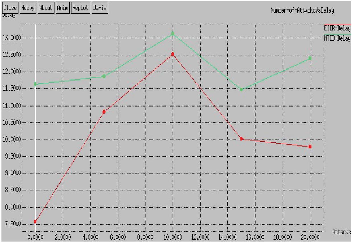
Figure 2 Delay comparisons with varying malicious nodes (single attack).
4.2.2 Case-1: Node density-100
In this test, we analyze the performance of EIDR with the fixed network size as 600 600 m area, node as 100 and varying the malicious nodes as 0, 5, 10, 15 and 20 for both single and multiple attacks.
The simulation time of this test is set as 500 seconds and compute performance metrics.
4.2.2.1 Single attack
Figure 2 shows the delay for both two schemes and it clearly depicts the delay of the proposed EIDR system is very lower than existing MITD scheme for different number of malicious nodes.
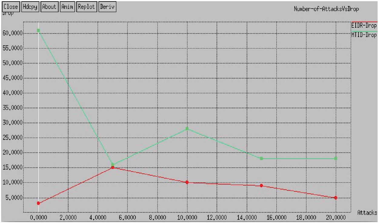
Figure 3 Packet loss rate comparisons with varying malicious nodes (single attack).
Figure 3 shows the packet loss ratio for both two schemes and it clearly depicts the loss ratio of the proposed EIDR system is lower than existing MITD scheme for different number of malicious nodes.
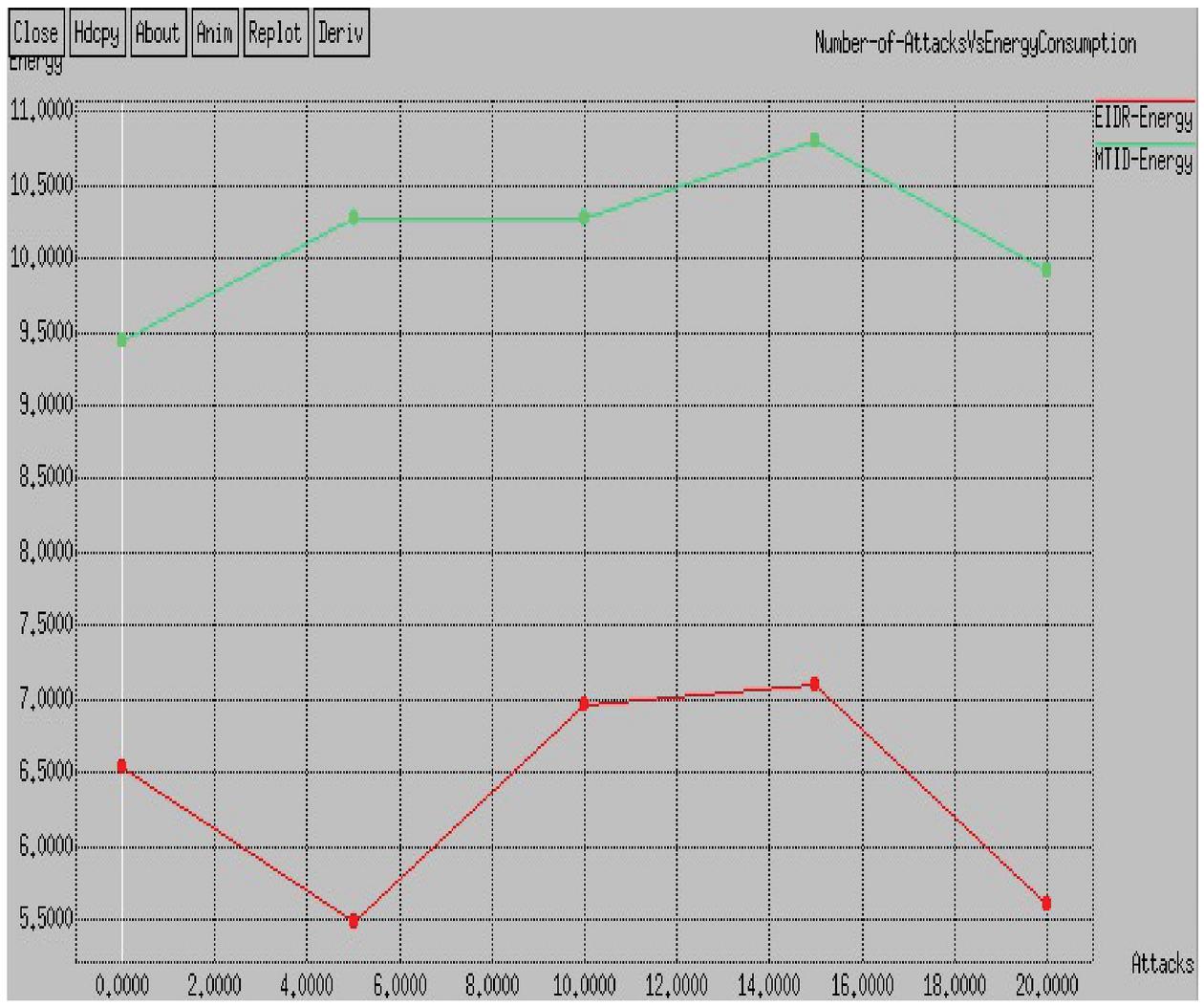
Figure 4 Energy consumption comparisons with varying malicious nodes (single attack).
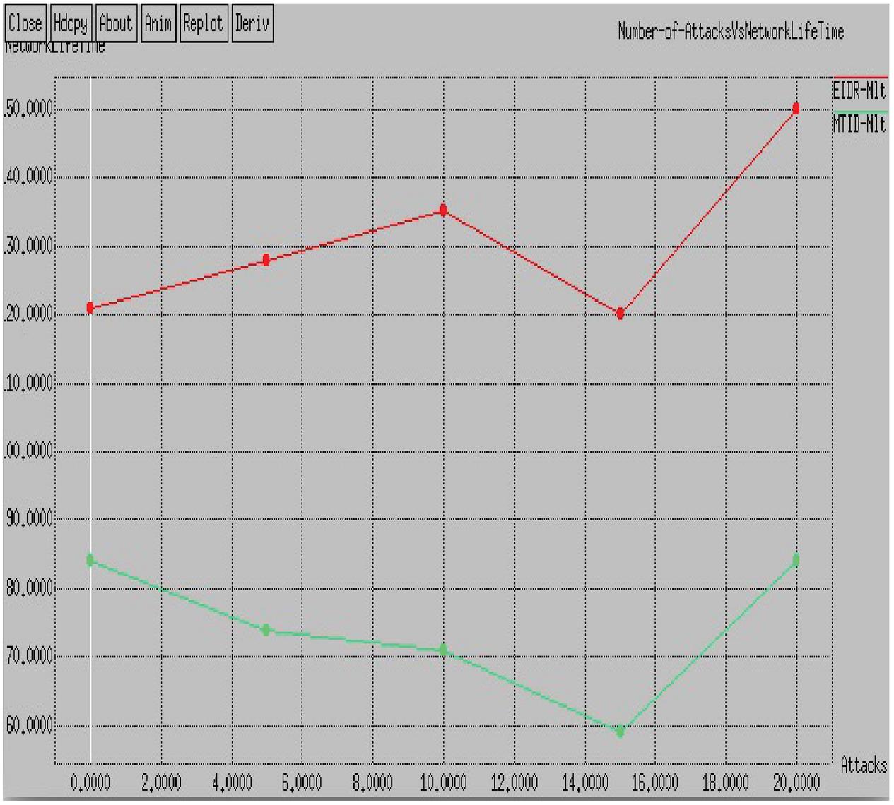
Figure 5 Network lifetime comparisons with varying malicious nodes (single attack).
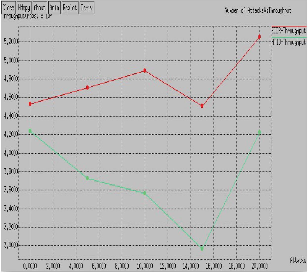
Figure 6 Throughput comparisons with varying malicious nodes (single attack).
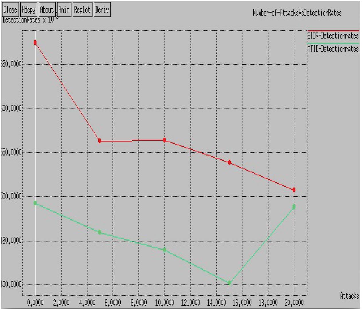
Figure 7 Detection rate comparisons with varying malicious nodes (single attack).
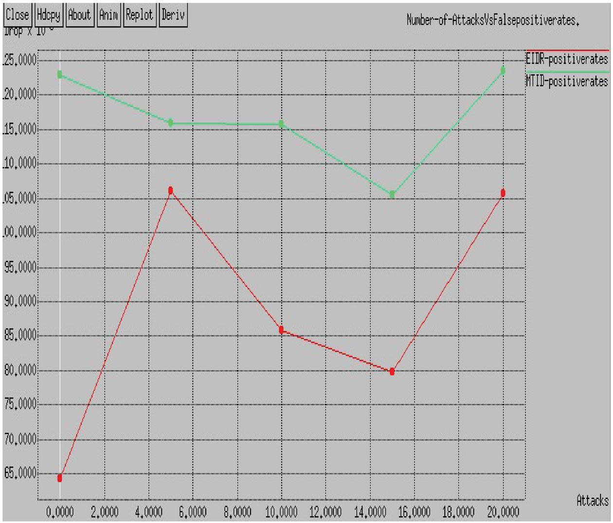
Figure 8 False positive rate comparisons with varying malicious nodes (single attack).
Figure 4 shows the energy consumption for both two schemes and it clearly depicts the energy consumption of the proposed EIDR system is very lower than existing MITD scheme for different number of malicious nodes.
Figure 5 shows the network lifetime for both two schemes and it clearly depicts the network lifetime of the proposed EIDR system is very higher than existing MITD scheme for different number of malicious nodes.
Figure 6 show the throughput for both two schemes and it clearly depicts the throughput of the proposed EIDR system is very higher than existing MITD scheme for different number of malicious nodes.
Figure 7 shows the detection rate for both two schemes and it clearly depicts the detection rate of the proposed EIDR system is very higher than existing MITD scheme for different number of malicious nodes. Figure 8 shows the false positive rate for both two schemes and it clearly depicts the false positive rate of the proposed EIDR system is very lower than existing MITD scheme for different number of malicious nodes.
4.2.2.2 Multiple attacks
Figure 9 shows the delay for both two schemes and it clearly depicts the delay of the proposed EIDR system is very lower than existing MITD scheme for different number of malicious nodes.
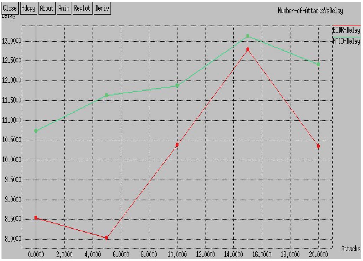
Figure 9 Delay comparisons with varying malicious nodes (multiple attacks).
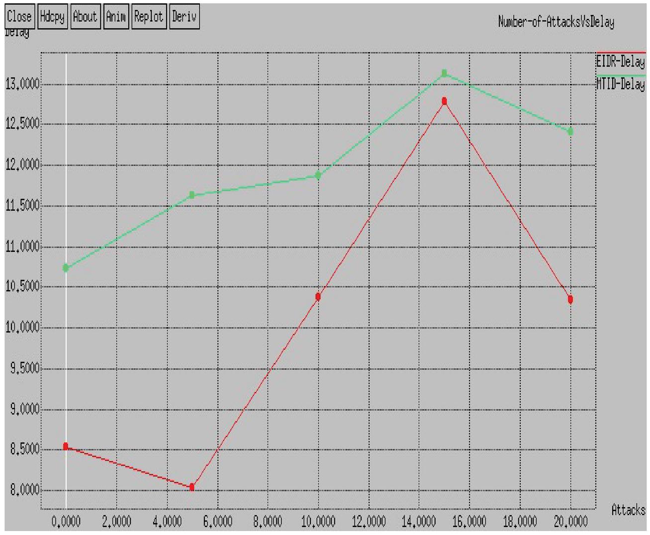
Figure 10 Packet loss rate comparisons with varying malicious nodes (multiple attacks).
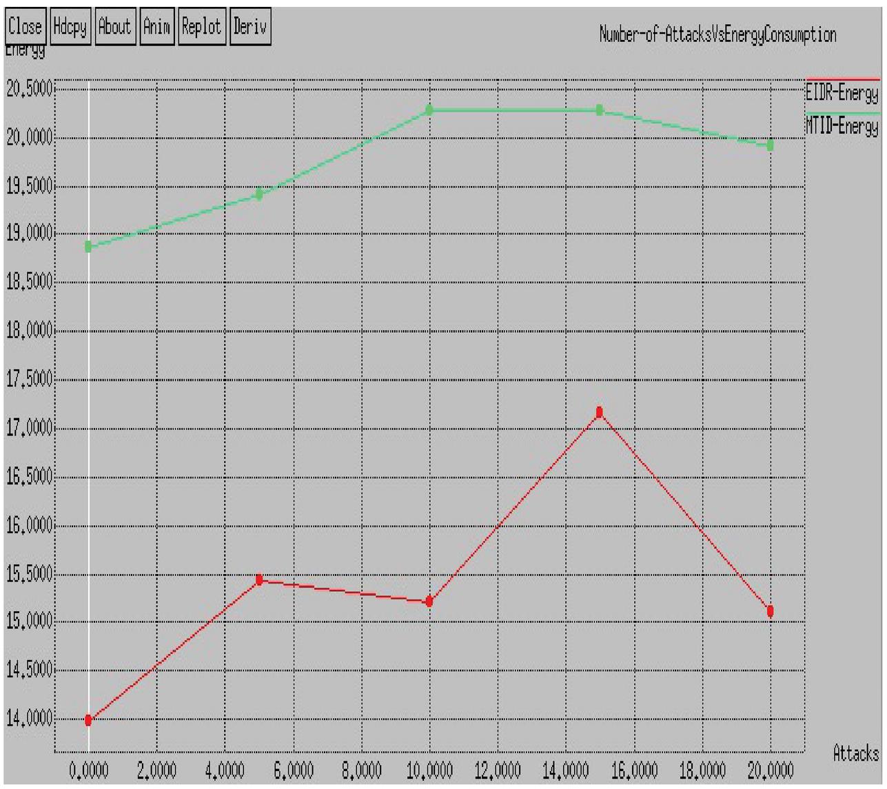
Figure 11 Energy consumption comparisons with varying malicious nodes (multiple attacks).
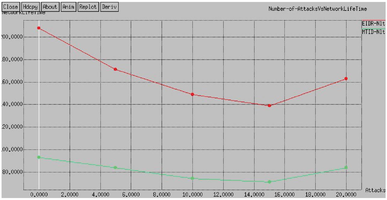
Figure 12 Network lifetime comparisons with varying malicious nodes (multiple attacks).
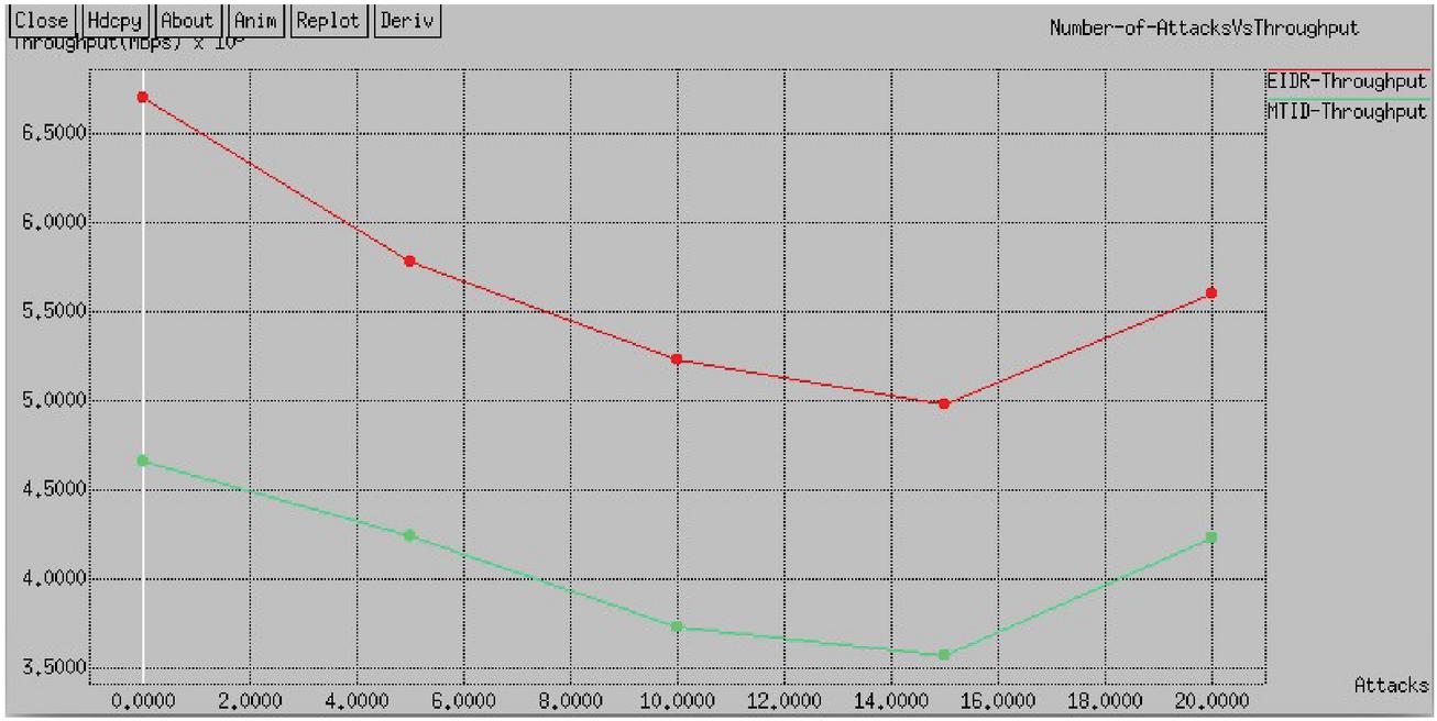
Figure 13 Throughput comparisons with varying malicious nodes (multiple attacks).
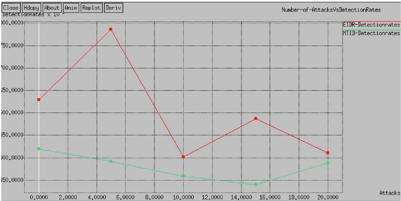
Figure 14 Detection rate comparisons with varying malicious nodes (multiple attacks).
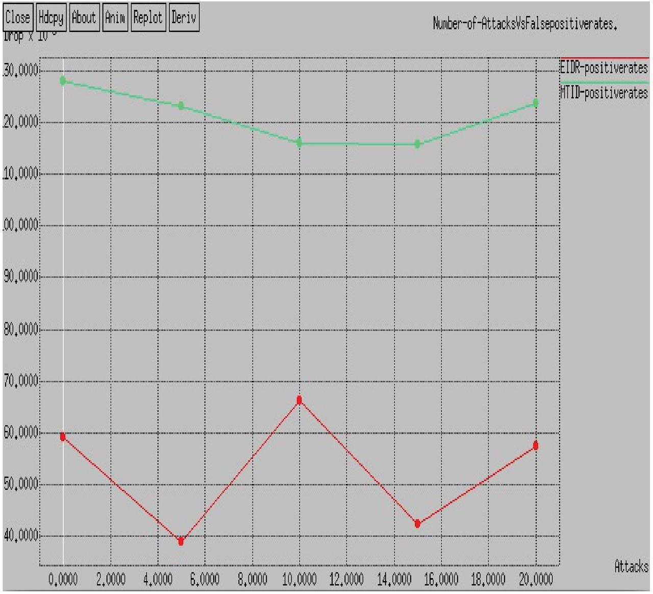
Figure 15 False positive rate comparisons with varying malicious nodes (multiple attacks).
Figure 10 shows the packet loss ratio for both two schemes and it clearly depicts the loss ratio of the proposed EIDR system is lower than existing MITD scheme for different number of malicious nodes.
Figure 11 shows the energy consumption for both two schemes and it clearly depicts the energy consumption of the proposed EIDR system is very lower than existing MITD scheme for different number of malicious nodes.
Figure 12 shows the network lifetime for both two schemes and it clearly depicts the network lifetime of the proposed EIDR system is very higher than existing MITD scheme for different number of malicious nodes. Figure 13 show the throughput for both two schemes and it clearly depicts the throughput of the proposed EIDR system is very higher than existing MITD scheme for different number of malicious nodes. Figure 14 shows the detection rate for both two schemes and it clearly depicts the detection rate of the proposed EIDR system is very higher than existing MITD scheme for different number of malicious nodes. Figure 15 shows the false positive rate for both two schemes and it clearly depicts the false positive rate of the proposed EIDR system is very lower than existing MITD scheme for different number of malicious nodes.
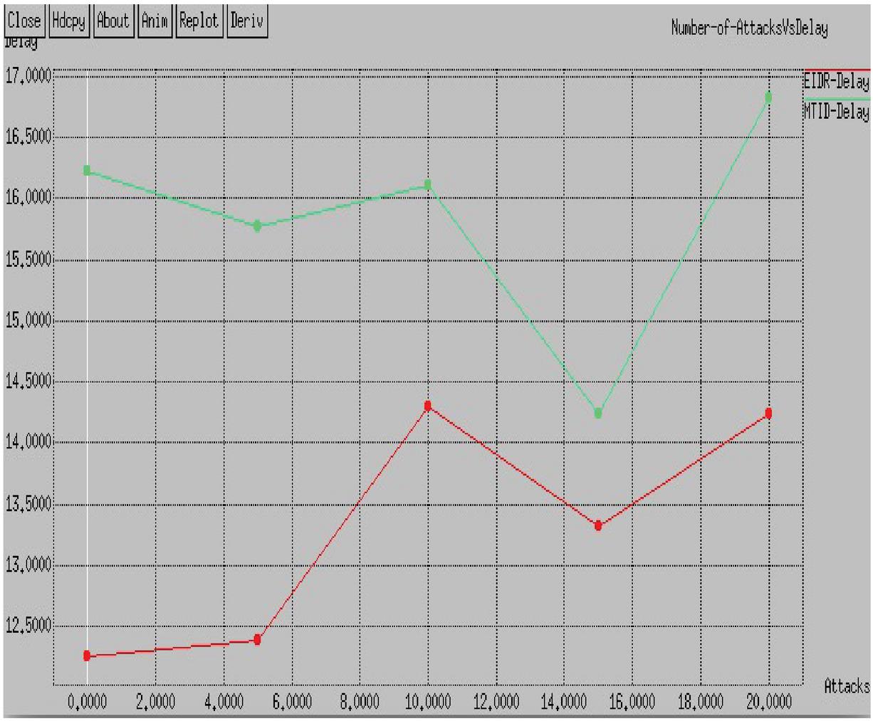
Figure 16 Delay comparisons with varying malicious nodes (single attack).
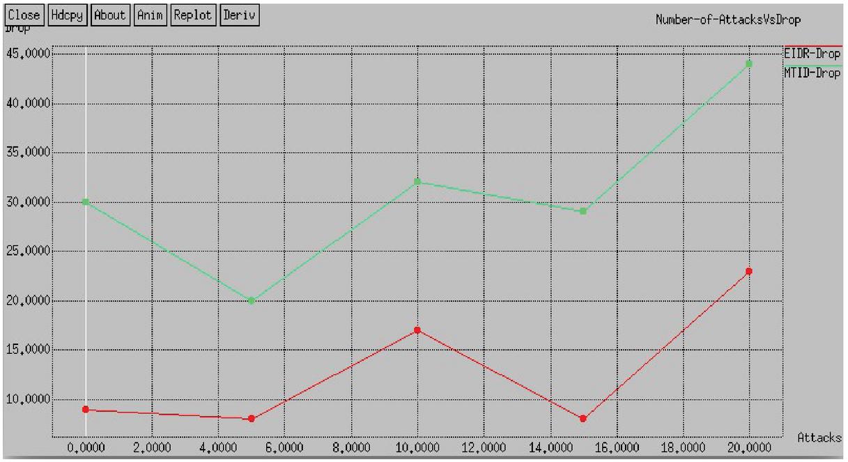
Figure 17 Packet loss rate comparisons with varying malicious nodes (single attack).
4.2.2.3 Case-2: Node density-200
In this test, we analyze the performance of EIDR with the fixed network size as 300 300 m area, node as 200 and varying the malicious nodes as 0, 5, 10, 15 and 20 (single attack). The simulation time of this test is set as 100 seconds and compute performance metrics. Figure 16 shows the delay for both two schemes and it clearly depicts the delay of the proposed EIDR system is very lower than existing MITD scheme.
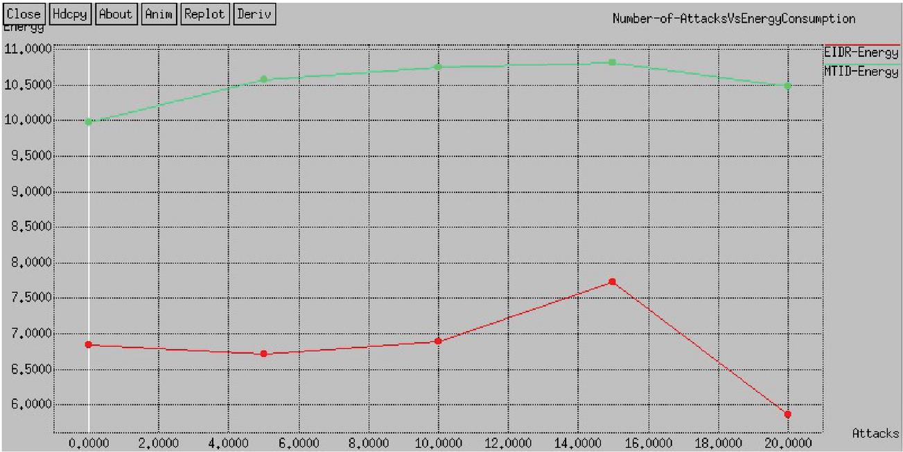
Figure 18 Energy consumption comparisons with varying malicious nodes (single attack).
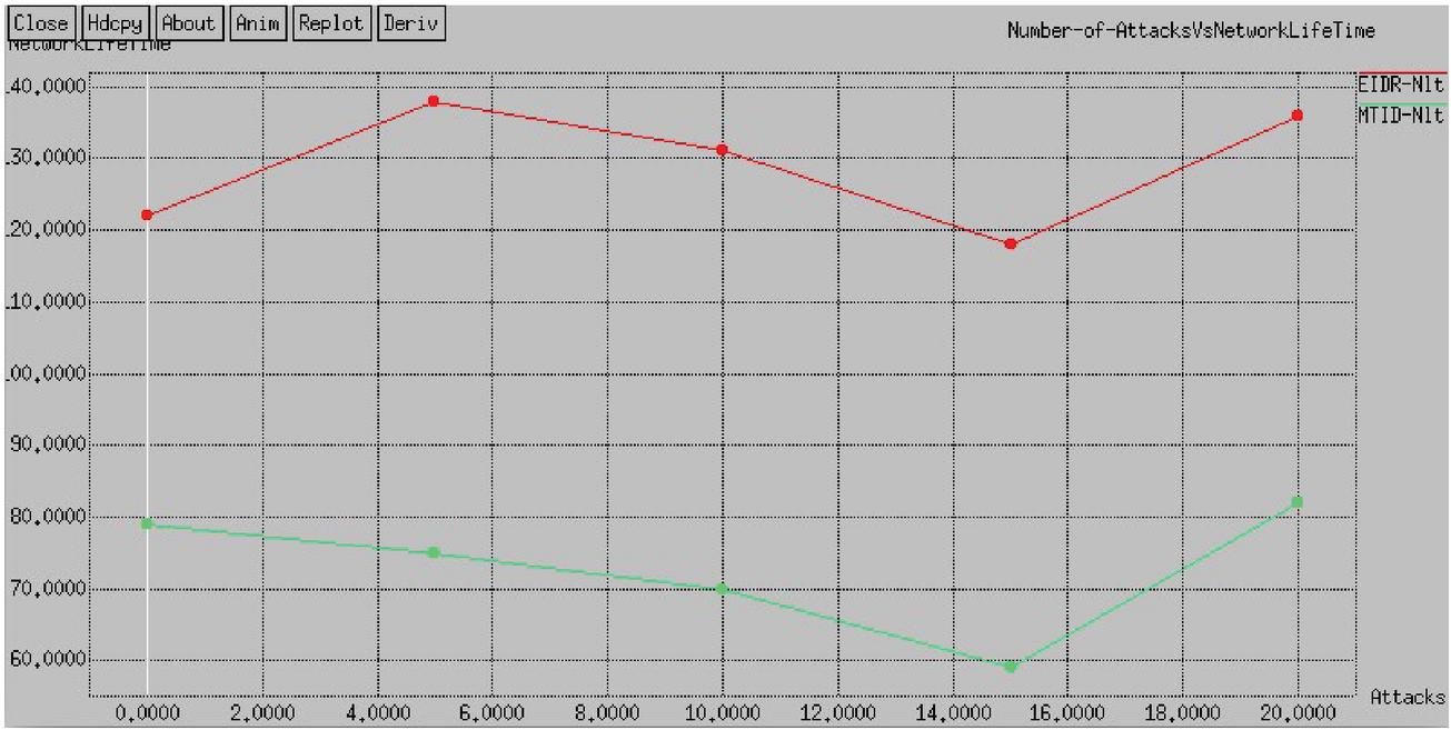
Figure 19 Network lifetime comparison with varying malicious nodes (single attack).
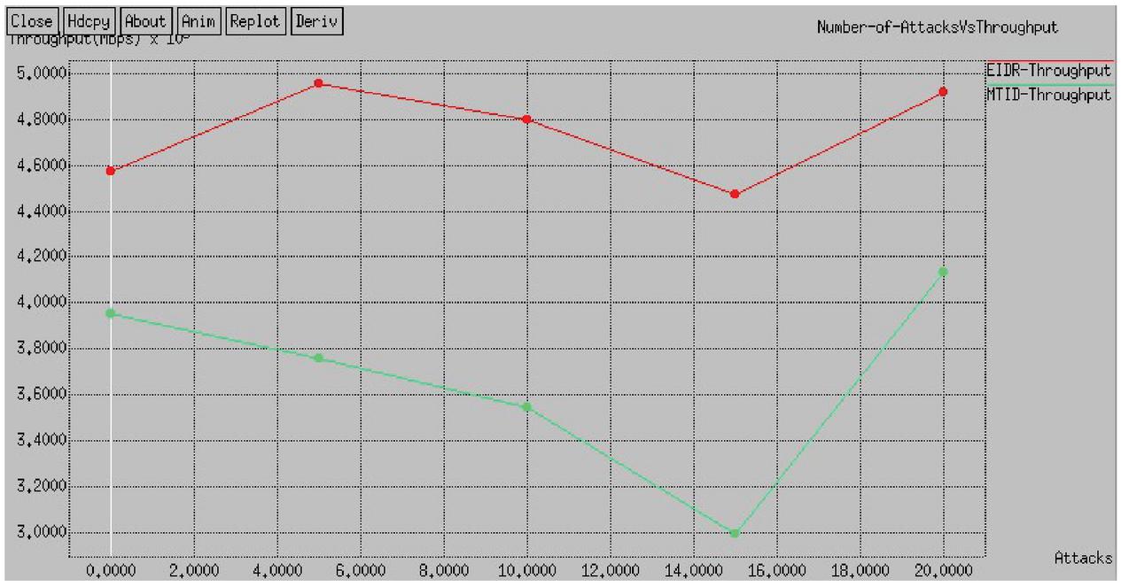
Figure 20 Throughput comparisons with varying malicious nodes (single attack).
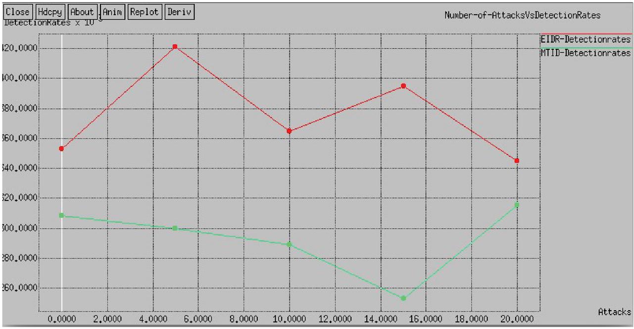
Figure 21 Detection rate comparisons with varying malicious nodes (single attack).
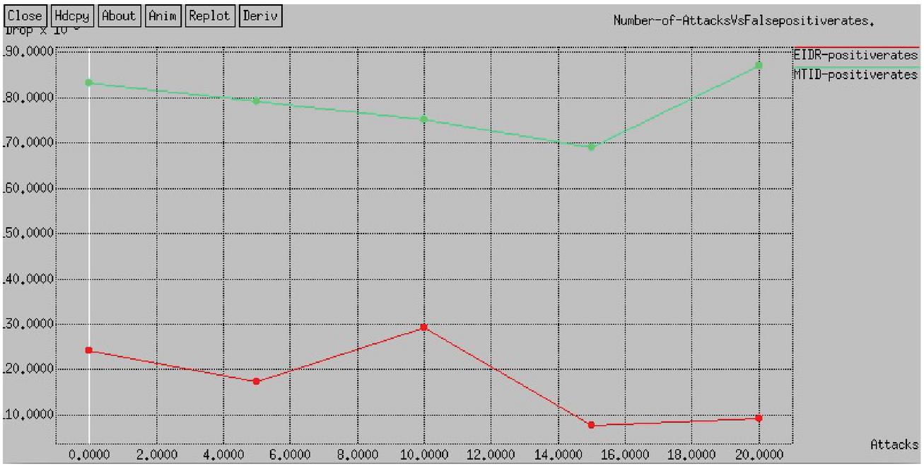
Figure 22 False positive rate comparisons with varying malicious nodes (single attack).
Figure 17 shows the packet loss ratio for both two schemes and it clearly depicts the loss ratio of the proposed EIDR system is lower than existing MITD scheme. Figure 18 shows the energy consumption for both two schemes and it clearly depicts the energy consumption of the proposed EIDR system is very lower than existing MITD scheme. Figure 19 shows the network lifetime for both two schemes and it clearly depicts the network lifetime of the proposed EIDR system is very higher than existing MITD scheme. Figure 20 show the throughput for both two schemes and it clearly depicts the throughput of the proposed EIDR system is very higher than existing MITD scheme for different number of malicious nodes.
Figure 21 shows the detection rate for both two schemes and it clearly depicts the detection rate of the proposed EIDR system is very higher than existing MITD scheme. Figure 22 shows the false positive rate for both two schemes and it clearly depicts the false positive rate of the proposed EIDR system is very lower than existing MITD scheme.
5 Conclusion
We have proposed an enhanced intrusion detection and response (EIDR) system using the combination of clustering and trust model. In EIDR, chaotic ant optimization (CAO) algorithm is utilized to form the optimal clustering with balanced network and multi objective differential evolution (MODE) algorithm is utilized to compute the trust value of each node. Then, perform the intrusion response action (IRA) system using the computed trust values. The simulation result shows the effectiveness of proposed EIDR system in terms of delay, loss ratio, energy consumption, network lifetime, throughput, detection rate and false positive rate.
References
[1] A. Bleda, F. Fernandez-Luque, A. Rosa, J. Zapata and R. Maestre, “Smart Sensory Furniture Based on WSN for Ambient Assisted Living”, IEEE Sensors Journal, vol. 17, no. 17, pp. 5626–5636, 2017.
[2] J. Wu, K. Ota, M. Dong and C. Li, “A Hierarchical Security Framework for Defending Against Sophisticated Attacks on Wireless Sensor Networks in Smart Cities”, IEEE Access, vol. 4, pp. 416–424, 2016.
[3] S. Jokhio, I. Jokhio and A. Kemp, “Light-weight framework for security-sensitive wireless sensor networks applications”, IET Wireless Sensor Systems, vol. 3, no. 4, pp. 298–306, 2013.
[4] F. Valeur, G. Vigna, C. Kruegel and R. Kemmerer, “Comprehensive approach to intrusion detection alert correlation”, IEEE Transactions on Dependable and Secure Computing, vol. 1, no. 3, pp. 146–169, 2004.
[5] A. Mishra, K. Nadkarni and A. Patcha, “Intrusion detection in wireless ad hoc networks”, IEEE Wireless Communications, vol. 11, no. 1, pp. 48–60, 2004.
[6] N. Ye, Q. Chen and C. Borror, “EWMA Forecast of Normal System Activity for Computer Intrusion Detection”, IEEE Transactions on Reliability, vol. 53, no. 4, pp. 557–566, 2004.
[7] R. Erbacher, K. Walker and D. Frincke, “Intrusion and misuse detection in large-scale systems”, IEEE Computer Graphics and Applications, vol. 22, no. 1, pp. 38–47, 2002.
[8] B. Hoyle, M. Rau, K. Paech, C. Bonnett, S. Seitz and J. Weller, “Anomaly detection for machine learning redshifts applied to SDSS galaxies”, Monthly Notices of the Royal Astronomical Society, vol. 452, no. 4, pp. 4183–4194, 2015.
[9] B. Sun, L. Osborne, Y. Xiao and S. Guizani, “Intrusion detection techniques in mobile ad hoc and wireless sensor networks”, IEEE Wireless Communications, vol. 14, no. 5, pp. 56–63, 2007.
[10] Yun Wang, Xiaodong Wang, Bin Xie, Demin Wang and D. Agrawal, “Intrusion Detection in Homogeneous and Heterogeneous Wireless Sensor Networks”, IEEE Transactions on Mobile Computing, vol. 7, no. 6, pp. 698–711, 2008.
[11] S. Shin, T. Kwon, G. Jo, Y. Park and H. Rhy, “An Experimental Study of Hierarchical Intrusion Detection for Wireless Industrial Sensor Networks”, IEEE Transactions on Industrial Informatics, vol. 6, no. 4, pp. 744–757, 2010.
[12] S. Bu, F. Yu, X. Liu and H. Tang, “Structural Results for Combined Continuous User Authentication and Intrusion Detection in High Security Mobile Ad-Hoc Networks”, IEEE Transactions on Wireless Communications, vol. 10, no. 9, pp. 3064–3073, 2011.
[13] F. Bao, I. Chen, M. Chang and J. Cho, “Hierarchical Trust Management for Wireless Sensor Networks and its Applications to Trust-Based Routing and Intrusion Detection”, IEEE Transactions on Network and Service Management, vol. 9, no. 2, pp. 169–183, 2012.
[14] M. Wei and K. Kim, “Intrusion detection scheme using traffic prediction for wireless industrial networks”, Journal of Communications and Networks, vol. 14, no. 3, pp. 310–318, 2012.
[15] J. Chen, J. Li and T. Lai, “Energy-Efficient Intrusion Detection with a Barrier of Probabilistic Sensors: Global and Local”, IEEE Transactions on Wireless Communications, vol. 12, no. 9, pp. 4742–4755, 2013.
[16] A. Abduvaliyev, A. Pathan, Jianying Zhou, R. Roman and Wai-Choong Wong, “On the Vital Areas of Intrusion Detection Systems in Wireless Sensor Networks”, IEEE Communications Surveys & Tutorials, vol. 15, no. 3, pp. 1223–1237, 2013.
[17] B. Sun, X. Shan, K. Wu and Y. Xiao, “Anomaly Detection Based Secure In-Network Aggregation for Wireless Sensor Networks”, IEEE Systems Journal, vol. 7, no. 1, pp. 13–25, 2013.
[18] V. Matyas and J. Kur, “Conflicts between Intrusion Detection and Privacy Mechanisms for Wireless Sensor Networks”, IEEE Security & Privacy, vol. 11, no. 5, pp. 73–76, 2013.
[19] G. Han, J. Rodrigues, J. Jiang, L. Shu and W. Shen, “IDSEP: a novel intrusion detection scheme based on energy prediction in cluster-based wireless sensor networks”, IET Information Security, vol. 7, no. 2, pp. 97–105, 2013.
[20] H. Moosavi and F. Bui, “A Game-Theoretic Framework for Robust Optimal Intrusion Detection in Wireless Sensor Networks”, IEEE Transactions on Information Forensics and Security, vol. 9, no. 9, pp. 1367–1379, 2014.
[21] G. Han, X. Li, J. Jiang, L. Shu and J. Lloret, “Intrusion Detection Algorithm Based on Neighbor Information Against Sinkhole Attack in Wireless Sensor Networks”, The Computer Journal, vol. 58, no. 6, pp. 1280–1292, 2014.
[22] K. Lin, T. Xu, J. Song, Y. Qian and Y. Sun, “Node Scheduling for All-Directional Intrusion Detection in SDR-Based 3D WSNs”, IEEE Sensors Journal, vol. 16, no. 20, pp. 7332–7341, 2016.
[23] C. Pintea, P. Pop and I. Zelina, “Denial jamming attacks on wireless sensor network using sensitive agents”, Logic Journal of IGPL, p. jzv046, 2015.
[24] K. Huang, Q. Zhang, C. Zhou, N. Xiong and Y. Qin, “An Efficient Intrusion Detection Approach for Visual Sensor Networks Based on Traffic Pattern Learning”, IEEE Transactions on Systems, Man, and Cybernetics: Systems, vol. 47, no. 10, pp. 2704–2713, 2017.
[25] Z. Zhang, H. Zhu, S. Luo, Y. Xin and X. Liu, “Intrusion Detection Based on State Context and Hierarchical Trust in Wireless Sensor Networks”, IEEE Access, vol. 5, pp. 12088–12102, 2017.
[26] K. Mrugala, N. Tuptuk and S. Hailes, “Evolving attackers against wireless sensor networks using genetic programming”, IET Wireless Sensor Systems, vol. 7, no. 4, pp. 113–122, 2017.
[27] H. Sedjelmaci, S. Senouci and N. Ansari, “Intrusion Detection and Ejection Framework Against Lethal Attacks in UAV-Aided Networks: A Bayesian Game-Theoretic Methodology”, IEEE Transactions on Intelligent Transportation Systems, vol. 18, no. 5, pp. 1143–1153, 2017.
[28] Q. Guo, X. Li, G. Xu and Z. Feng, “MP-MID: Multi-Protocol Oriented Middleware-level Intrusion Detection method for wireless sensor networks”, Future Generation Computer Systems, vol. 70, pp. 42–47, 2017.
[29] D. Santoro, G. Escudero-Andreu, K. Kyriakopoulos, F. Aparicio-Navarro, D. Parish and M. Vadursi, “A hybrid intrusion detection system for virtual jamming attacks on wireless networks”, Measurement, vol. 109, pp. 79–87, 2017.
[30] N. Alsaedi, F. Hashim, A. Sali and F. Rokhani, “Detecting sybil attacks in clustered wireless sensor networks based on energy trust system (ETS)”, Computer Communications, vol. 110, pp. 75–82, 2017.
[31] X. Jin, J. Liang, W. Tong, L. Lu and Z. Li, “Multi-agent trust-based intrusion detection scheme for wireless sensor networks”, Computers & Electrical Engineering, vol. 59, pp. 262–273, 2017.
[32] D. Deif and Y. Gadallah, “An Ant Colony Optimization Approach for the Deployment of Reliable Wireless Sensor Networks”, IEEE Access, vol. 5, pp. 10744–10756, 2017.
[33] H. Harno and I. Petersen, “Synthesis of Linear Coherent Quantum Control Systems Using A Differential Evolution Algorithm”, IEEE Transactions on Automatic Control, vol. 60, no. 3, pp. 799–805, 2015.
Biographies

A. Kathirvel, acquired, B.E.(CSE), M.E. (CSE) from University of Madras and Ph. D (CSE.) from Anna University. He has served in various positions at Deemed Universities, Autonomous Institution and Anna University affiliated colleges from 1998 to till date. He is currently working as Professor, Dept of Computer Science and Engineering, SRM Institute of Science and Technology, Vadapalani Campus at Chennai. He has worked as Lecturer, Senior Lecturer, Assistant Professor, Professor, and Professor & Head in various institutions. He is a studious researcher by himself, completed 18 sponsored research projects worth of Rs 103 lakhs and published more than 110 articles in journals and conferences. 4 research scholars have completed Ph. D and 3 under progress under his guidance.He is working as scientific and editorial board member of many journals. He has reviewed dozens of papers in many journals. He has author of 12 books. His research interests are protocol development for wireless ad hoc networks, security in ad hoc network, data communication and networks, mobile computing, wireless networks and Delay tolerant networks.

M. Subramaniam (1974) is a Professor, in Department of Computer Science and Engineering, School of Computing, SRM Institute of Science and Technology (Deemed to be University u/s 3 of UGC Act, 1956) – Vadapalani Campus, Chennai-600026, (INDIA). He obtained his Bachelor’s degree (B.E) in Computer Science and Engineering from University of Madras (1998), Master degree (M.E) in Software Engineering and Ph.D from College of Engineering Guindy (CEG), Anna University Main Campus, Chennai-25 in the year 2003 and 2013 respectively. His research focuses are Computer Networks, Software Engineering, AI & ML. He is an active life member of the Computer Society of India (CSI), the Indian Society for Technical Education (ISTE) and International Association of Engineers (IAENG). He has produced one doctorate and currently seven research scholars perusing Ph.D under his guidance. He has published many research papers in reputed journals. He is also reviewer in Springer-WPC, IEEE International Journal of Communication Systems.
C. Sabarinathan, Assistant Professor, Department of CSE, Faculty of Engineering and Technology, SRM Institute of Science and Technology, Vadapalani Campus, Chennai, Tamilnadu, India.
S. Navaneethan, Research Scholar, Department of CSE, Faculty of Engineering and Technology, SRM Institute of Science and Technology, Vadapalani Campus, Chennai, Tamilnadu, India.
Journal of Web Engineering, Vol. 20_1, 53–88.
doi: 10.13052/jwe1540-9589.2013
© 2021 River Publishers