Intelligent Model-based Integrity Assessment of Nonstationary Mechanical System
Hanxin Chen1, 2, *, Yuzhuo Miao1, Yongting Chen3, Lu Fang1, Li Zeng1 and Jun Shi1
1School of Mechanical and Electrical Engineering Wuhan Institute of Technology, Wuhan 430073, China
2School of Artificial Intelligence, Nanchang Institute of Science and Technology, Nanchang, 330108, China
3Wuhan Britain-China School, Wuhan, China
E-mail: pg01074075@163.com
*Corresponding Author
Received 20 October 2020; Accepted 18 November 2020; Publication 05 March 2021
Abstract
The fault diagnosis model for nonstationary mechanical system is proposed in the condition monitoring. The algorithm with an improved particle filter and Back Propagation for intelligent fault identification is developed, which is used to reduce the noise of the experimental vibration signals to delete the negative effect of the noise on the feature extraction of the original vibration signal. The proposed integrated method is applied for the trouble shoot of the impellers inside the centrifugal pump. The principal component analysis (PCA) method optimizes the clean vibration signal to choose the optimal eigenvalue features.The constructed (back propagation)BP neural network is trained to get the condition models for fault identification. The proposed novel model is compared with the BP neural network based on traditional PF and particle swarm optimization particle filter (PSO-PF) algorithm. The BP neural network diagnosis method based on the improved PF algorithm is much better for the integrity assessment of the centrifugal pump impeller. This method is much significant for big data mining in the fault diagnosis method of the complex mechanical system.
Keywords: Integrity assessment, nonstationary mechanical system, model-based, improved particle filter.
1 Introduction
As we all know, the health management of machinery and equipment has an indispensable importance in the development of industrial modernization. The current research progress of the artificial intelligence is extremely rapid, the industry 4.0 era is also coming soon. Mechanical equipment will also develop in the direction of high integration, high precision and intelligence, and the correlation and complexity between mechanical equipment will be greatly increased [1–3]. Therefore, when structural defects or other failures occur in mechanical equipment, changes such as physical and chemical factors occur. At the same time, when conducting online monitoring of the equipment, it is faced with the problems of a wide variety of collected data, noise and interference [4–7]. Under the background of such machinery-related big data, to realize online health monitoring of the entire mechanical equipment, a mechanical fault diagnosis method suitable for processing data signals is needed. Centrifugal pumps are very important equipment for industrial production and play a vital role in the entire industrial economy. For energy conversion, fluid transfer, etc., centrifugal pumps are one of the main devices [8]. Among them, the working environment of the impeller of the centrifugal pump is relatively poor, because it is in direct contact with the transmission material such as fluid, and the impeller is most susceptible to damage and corrosion after working for a long time. When the impeller is damaged, the centrifugal pump will also reduce its life. If it is not discovered and repaired in time, a major accident is likely to occur [9, 10]. Then the impeller, an important part of the centrifugal pump, has high practical significance for its fault diagnosis research.
Generally, centrifugal pumps work in a relatively poor environment. When the impeller has abnormal vibration and noise, we can judge that the impeller is malfunctioning. For fault identification, the excitation signal is generally used to identify, and then the received signal is processed accordingly to decrease the interference of yawp to the vane wheel malfunction identification [11]. Commonly used noise elimination methods include wavelet analysis, empirical mode decomposition, and independent component analysis. These algorithms face the problem of complex parameter optimization choices in industrial production applications. For example, based on the wavelet base in the wavelet noise elimination method, the number of decomposition layers, and the choice of the threshold variables has the significant influence on the signal noise elimination effect. Usually there are many practical algorithms for processing nonlinear signals, and particle filtering is one of them. The algorithm has structural problems such as low computational efficiency, so the binding of PSO method and PF method has been extensively studied. The delegate of intelligent particle filter method is to introduce genetic mutation algorithm into PF algorithm for sampling processing [12]. In this paper, the genetic mutation algorithm and PSO algorithm are combined to optimize the defect of PSO algorithm which is apt to lapse into local extremum. The optimized PSO is introduced into the sampling process of PF algorithm to form an novel PF method. This algorithm is applied to fault diagnosis of centrifugal pump due to its high computational efficiency and accuracy.
Principal component analysis (PCA) is often applied in the reduced-dimension of data and selection of characteristic variables. In Li et al. [13], the principal component analysis is used in feature vectors of the relevant function to identify the structural condition, and multiple flaw detection are performed in the numerical model of a certain conduit. The results show that the method has better detection ability in different fault states with the different identification rates for the different fault locations and severity. Asghar et al. [14] proposed a techniques of applying PCA of Hotelling T index to fault detection and diagnosis in the production process, and combined it with matlab for verification. The results show that this method has high reliability for steady-state and transient fault detection. The PCA algorithm is combined with the BP neural network. Cadini et al. [15] proposed the flexibility provided by traditional particle filters and neural networks to learn adaptively and in real time from monitored structures, and to derive models for diagnosing and predicting structural components affected by the damage process, and to observe the damage process of mechanical components. This paper adopts the method of combining PCA algorithm and BP neural network model. Firstly, PCA algorithm is suitable for reducing the dimension of characteristic variables, and then the BP neural network model is applied to identify the fault types. Finally, the constructed diagnostic model and diagnostic accuracy were provided by four-fold cross-validation.
For preventing the problem of the PF method about less sampling in the later sampling period, this paper calculates the PSO with mutation operator in PF sampling, optimize the PF algorithm, and improve the accuracy and convergence speed. The algorithm reduces the noise of vibration signals for four different impeller faults. The PCA algorithm reduces the time-domain feature value of the extracted data, so the amount of feature variables is decreased, so the neural network training speed is faster and the accuracy is higher. Then, impeller fault type is identified by BP neural network, the built diagnostic model and diagnostic accuracy are verified by quadruple cross-validation. By comparing with a control group based on two different noise elimination methods, proved that the method combining the PSO algorithm and the PE algorithm is effective for diagnosing impeller faults of centrifugal pumps, and the method also has a fast diagnosis speed And high accuracy, which also shows this method is suitable for more complicated mechanical fault diagnosis.
2 PSO-PF Algorithms with Mutation Operation
2.1 PSO Algorithms with Variation Operation
The PSO algorithms is a random search algorithm that was first put forward by Kennedy and Eberhart in 1995 to simulate the foraging behavior of birds [21]. In an n-dimension spacewith number of particles. The particle i contains multiple parameters, such as speed position , individual extreme value , and overall global extreme value . Then the velocity and position of the particle can be expressed by the formula (1):
| (1) |
Where is a random number between interval , and are are learning factors, and . is the inertia coefficient.
Traditional particle swarm optimization algorithms often have the problem of local extremum, which is solved with the genetic algorithm mutation operator in the particle swarm optimization algorithm. The specific approach is to lead in a variation control function to control the number of particles of variation to maintain the diversity within the population, thereby avoiding premature convergence at the local optimum. The introduced variation control function is:
| (2) |
Where is the current iterations amount, is the maximum iterations amount, and are the control modulus.
Calculating the control rate of the variation control according to Equation (3):
| (3) |
Calculating the number of particles for the variation operation according to Equation (4):
| (4) |
According to the formula (4), the particles to be subjected to the mutation operation are randomly selected from the particle group and digitally encoded. Suppose the m-th particle is selected for mutation, such as with the mutation of the n-th element, then the formula is:
| (5) |
Where is an arbitrary number.
The calculation formula of dynamic inertia coefficient is:
| (6) |
Where and are the largest and the minimum inertia coefficient.
2.2 Optimization of PF Algorithm
This paper uses the PSO algorithm of variation calculation to optimize the PF algorithm for sampling processing, and the particle fitness value is used to make the distribution of the particle swarm more ideal and close to the actual state. The purpose is to improve the correctness rates and effectiveness of the filtering. The newest observations is inputted into the PF sampling process and. The fitness function of the PSO algorithms is defined as follows:
| (7) |
Where is the variance, is the observation, and is the predicted value.
| (8) |
The above are hypothetically selected nonlinear dynamic system state and observation equation models. Where is the system state vector at moment, is the observation. The and are the process and observation noise. The and are non-linear functions.
The optimization process about the PF algorithm are described as:
Step 1: The corresponding parameters of the original algorithm. At time , sample based on the profile. The number of original formations , learning rates and , inertia coefficient , particle speed and position and, max iterations , preset variation rate .
Step 2: Optimizing the particle swarm sample distribution. Calculating function according to formula (2). The mutation rate is calculated according to the Equation (3), the number of mutant particles is calculated basic for the Equation (4). Implementing the variation operation according to the Equation (5). Calculating the inertia coefficient according to Equation (6). Calculating the fitness value for each particle according to Equation (7) and comparing its individual extremum . If then . Solving the global optimal value , if then . Updating the speed and location of the particle basic for Equation (1). When the maximum iterations amount is reached or the individual extremum satisfies the determined threshold , obtain the output particle group . If not, need to repeat the second step.
Step 3: Calculating the weights to assess the importance. Sampling from . The calculation of the importance weight is:
| (9) |
The weight normalization formula is:
| (10) |
Step 4: Perform the sampling process again. According to the significant weight , a new set of particles in time is gained by anew from the collection , the updated particle weights are generated based on the equation .
Step 5: Conclusion. After passing the first few steps, the estimated sample set , state estimation calculation formula is:
| (11) |
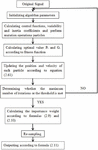
Figure 1 shows the specific operation flow of the algorithm.
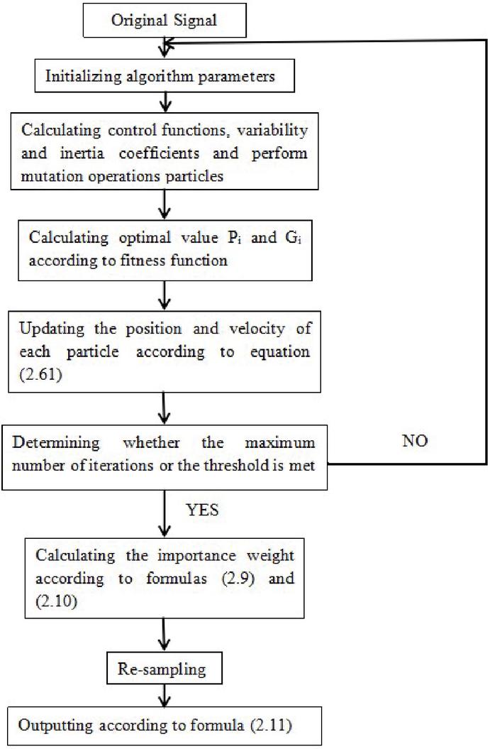
Figure 1 Algorithm flow diagram.
2.3 Noise Reduction Simulation Experiment
The noise reduction simulation experiment uses the following limit number, then the formula of the selected original signal is as follows:
| (12) |
According to formula (13), increase random noise signals of equal size:
| (13) |
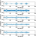
Equations (12) and (13) are used for replacing the state formula and the observation formula in Equation (8), separately, to form a space model of the simulation experiment system. The original density of probability function is , the original status value is 1, the observation noise variances , and the process noise variances . According to literature review and related experiments, the relevant parametrics of the PSO algorithm are: the number of particles , the fitness value . The number of iterations cannot exceed 200, and the variation control coefficients , the inertia weight , and the acceleration . Experimental simulations were performed on the number of ten particles of . Now the original signal map and noise reduction map (Figure 2) obtained by using PF, PSO-PF and (Novel Particle Swarm Optimization-Particle Filter) NPSO-PF noise reduction.
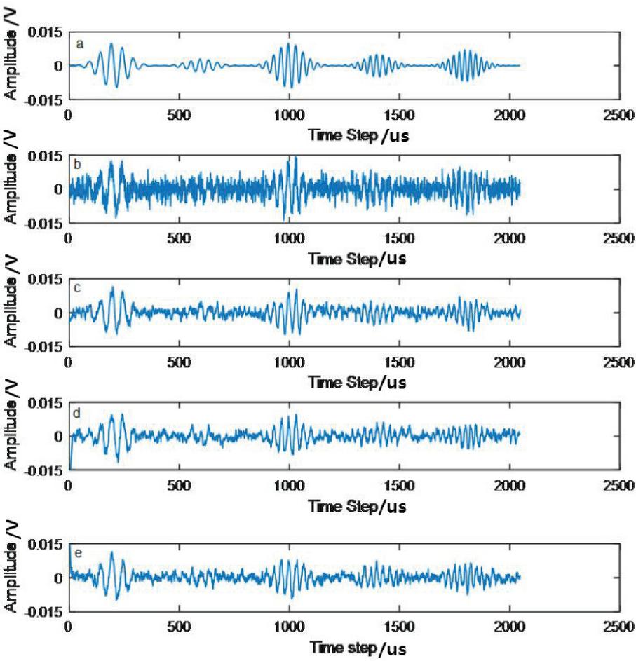
Figure 2 Simulation results of noise reduction.
Figure 2 shows the original signal, the original signal with noise, the noise reduction using the PF algorithm, the noise reduction by the PSO-PF algorithm, and the noise reduction image by the NPSO-PF algorithm from top to bottom. As can be seen from the figure, PF, PSO-PF and NPSO-PF algorithms all have good noise reduction results. Among them, the third algorithm has the best effect after noise reduction. The smaller the SNR value, the worse the noise elimination effect. The average of the signal-to-noise ratios of the three algorithms is analyzed by the three algorithms of 50 noise reduction experiments. The simulation results are displayed in Table 2.1 and Figure 3. The calculation equation of the SNR is:
| (14) |
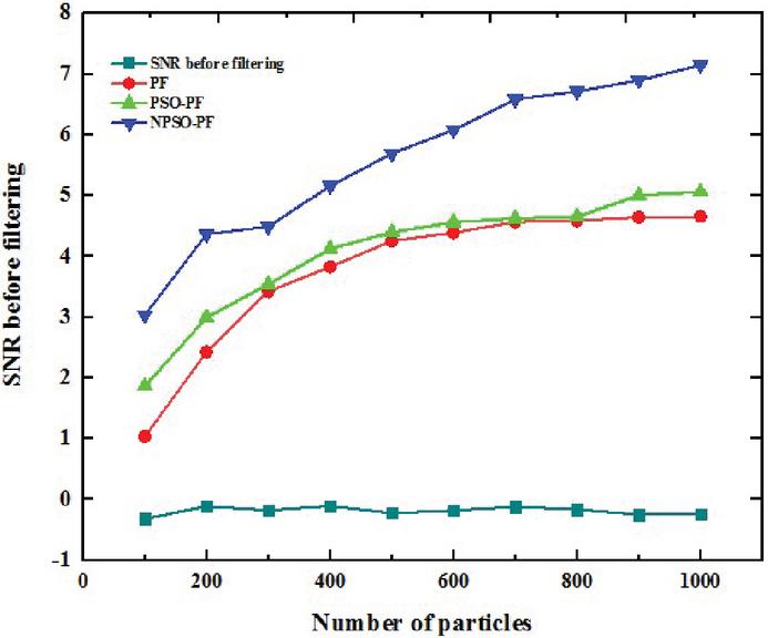
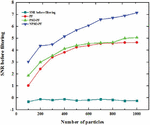
Figure 3 SNR after filtering.
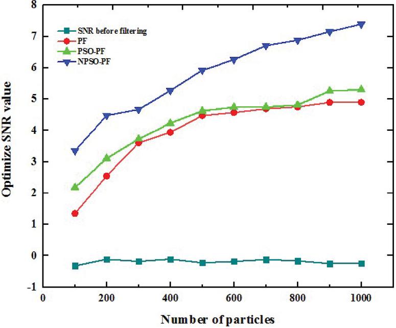
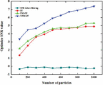
Figure 4 Optimize SNR value.
From Figures 3 and 4, it can be seen that compared with the SNR before filtering, compared with the SNR obtained by analyzing three algorithms of 10 kinds of particle swarm, all three methods are more effective. The PSO-PF method is a little better than PF method in noise reduction ability, but NPSO-PF method is the best. It can be observed from the two graphs that the noise reduction ability of the three algorithms increases with the increase of the quantity of particles. Among them, the noise reduction ability under the NPSO-PF algorithm is getting stronger and stronger, and the ability of the other two algorithms tends to be stable. Therefore, generally speaking, the noise decreased properties of NPSPO-PF method is more stable and reliable.
3 Test System and Data Preprocessing
3.1 Experimental System
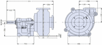
This article uses Weir/Warman3/2CAH mud pump. The impeller type of centrifugal pump is C2147, and its impeller has 5 blades. The mud pump size parameters used in the experiment are shown in Figure 5, in mm.
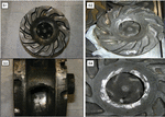
The experiments were performed by selecting ordinary impeller S1 and edge damaged impeller S2, blade damage impeller S3 and perforation damage impeller S4. The specific situation is shown in Figure 6.
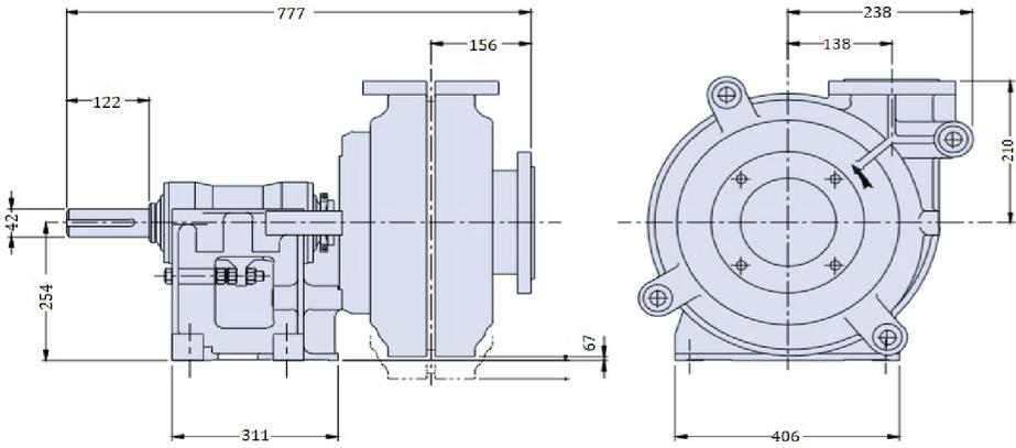
Figure 5 Centrifugal pump structure size.
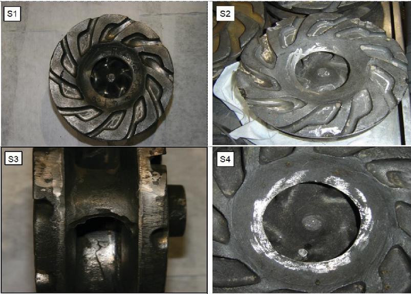
Figure 6 Impeller failure mode diagram.
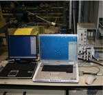
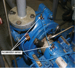
In this paper, the experiment mainly analyzes the multi-channel signals for instance oscillation, temperature, audio and pressure, and the data are stored by Dell 9200 computer. The test system has a fixed sampling frequency and frequency. The position of the sensor is shown in Figure 8. Three oscillation sensors are used to collect the data in actual time. The working fluid of this experiment is pure water. During this period, the experimental data of 2000 rpm running smoothly under four impeller conditions were recorded.

Figure 7 Signal acquisition system.
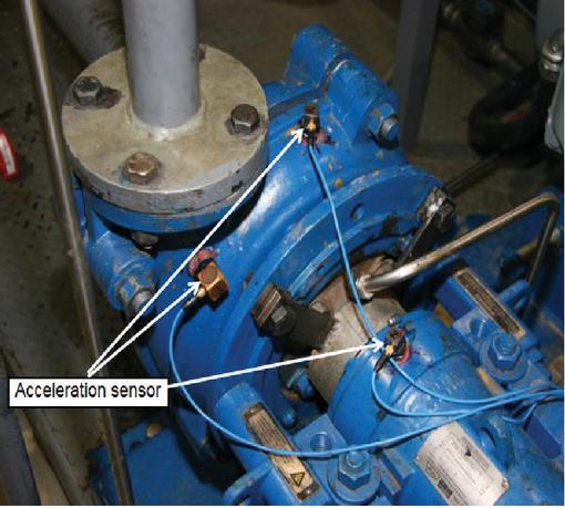
Figure 8 Acceleration sensor distribution point.
3.2 Noise Elimination of Experimental Data with NPSO-PF Algorithm
According to the principle of Nyquist sampling and analysis, the signal frequency analyzed in this paper is 4.5 KHz, and the acquisition time for each state of the impeller is 20 s. A total of nearly 180,000 data are obtained. In order to process the data more conveniently and better compare with the later stage The NPSO-PF method is used for data noise decrease processing for impellers in different states. According to the experiment and formula (2), nearly 180,000 data points are built into the following system model.
| (15) |
Where is time, is the simulated noise-free signal, is the signal measured at time , and and are Gaussian white noise with variances of and , respectively.
The particle number, initial state, initial state variance, process noise and state noise of the particle filter algorithm will all affect the performance of the filter. The parameters in the PSO method with mutation operator are the identical those in Section 2.3. The parameter settings for improved particle filtering are now determined according to multiple tests and references as shown in Table 1. The test raw data map is shown in Figure 9.
Table 1 Parameter settings for improved particle filtering
| Parameter | Numerical value |
| Initial state | |
| Initial probability density | |
| Process noise variance | |
| Measuring noise variance | |
| Number of particles | |
| Analog step size |
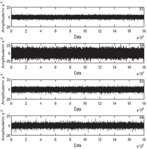
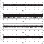
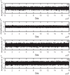
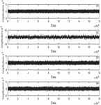
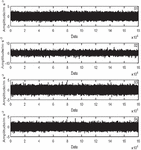
Figure 9 Original signal.
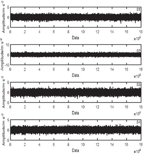
Figure 10 NPSO-PF noise elimination.
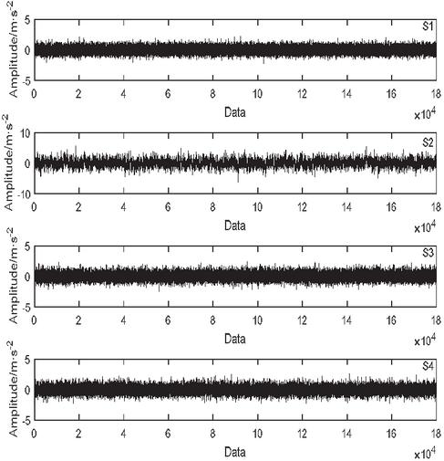
Figure 11 PSO-PF noise elimination.
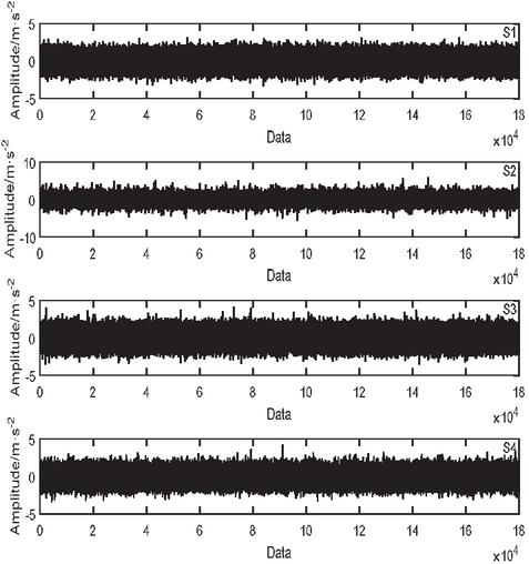
Figure 12 PF noise elimination.
The original signal of the experimental data and the signal after the noise reduction processing of the three algorithms are shown in Figures 9–12. It can be seen from this group of figures that the three noise reduction algorithms can effectively denoise the experimental vibration signal. The experimentally measured signals are nonlinear and cannot be represented by a specific formula. Therefore, the SNR analysis cannot be performed, and the noise elimination effects of the three algorithms cannot be quantified. It can be seen from the Figures that the amplitude of the data graph is reduced most with the NPSO-PF algorithm for noise elimination, and the graphics trend is clearer. Therefore, it can be shown what the NSPO-PF method has better noise decrease capabilities than the other two algorithms, and the denoised data will also provide a more accurate data basis for subsequent feature extraction and fault diagnosis.
4 Intelligent Diagnosis with PCA and BP
4.1 The Basic Theory About PCA Basic Principle for Optimal Features
The act of obtaining the required effective information from the received signal is usually called feature extraction, which can extract the effective eigenvalues of the signal, which not only makes the subsequent signal processing faster, but also makes the accuracy higher. The signal obtained in this study is the time-domain signal of vibration. Through the analysis of the time-domain signal, 13 time-domain statistical indexes such as mean, maximum, minimum, peak-to-peak, kurtosis factor and pulse index are extracted. After the analysis and processing of 13 characteristic variables by PCA, the speed and accuracy of BP neural network training and testing have been greatly improved. Divide the noise decrease data of each fault state into 40 units for analysis and treatment. The characteristic values in the normal impeller state obtained and normalized according to the time domain characteristics are shown in Table 2.
The principle of PCA counting hypothesis that the primitive data sample includes m n-dimensional eigenvectors. ; then the calculation steps are as follows:
Step 1: Calculating sample mean.
| (16) |
Step 2: Solving the eigenvalue and eigenvector of the sample vector covariance matrix .
| (17) |
Step 3: Calculating the contribution rate and the cumulative contribution rate of each principal element.
| (18) | |
| (19) |
Select the former element that the cumulative contribution rates match the standard of mapping matrices, and project the original data into the feature space:
| (20) |
Where .
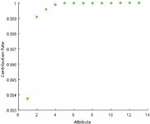
Based on the formula (20), the contribution rates of the principle element and the cumulative of the three methods after noise elimination are calculated. The main element contribution rate and cumulative contribution ratio are obtained by the denoised signal with the NPSO-PF algorithm and shown in Figure 13 and Table 2.
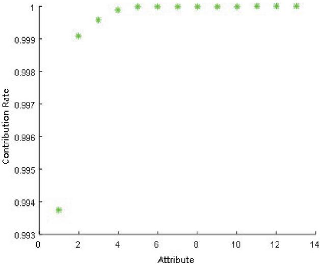
Figure 13 Principal component cumulative contribution rate after noise decrease by NPSO-PF method.
Table 2 Principal component contribution rate after noise decrease by NPSO-PF method
| Principal Number | Contribution Rate | Cumulative Contribution Rate |
| First principal | 99.38% | 99.38% |
| Second principal | 0.53% | 99.91% |
| Third principal | 0.05% | 99.96% |
| Fourth principal | 0.03% | 99.99% |
| Fifth principal | 0.01% | 100% |
| Sixth principal | 0 | 100% |
| Seventh principal | 0 | 100% |
| Eighth principal | 0 | 100% |
| Ninth principal | 0 | 100% |
| Tenth principal | 0 | 100% |
| Eleventh principal | 0 | 100% |
| Twelfth principal | 0 | 100% |
| Thirteenth principal | 0 | 100% |
For the limitation space, this article only gives the principal component contribution rate of NPSO-PF algorithm after noise reduction, and then uses PCA to analyze the signal after noise reduction. From the results, after the signal is processed by NPSO-PF algorithm, the contribution rate of the first principal component is as high as 99.38%, and the first principal component contribution rate is the highest among the three methods, and the signal processed by the NPSO-PF method is analyzed by PCA, and the first five principal components contain all the information of the signal. The results show that NPSO-PF method has the strongest noise decrease ability, which not only improves the effectiveness of PCA analysis, but also improves the speed and precision of data treatment. From the results of principal component analysis after NPSO-PF and PSO-PF noise elimination, it can be known that the first five principal components contain all the information of the original data, and the difference lies in the contribution ratio of each principal component. The principal component analysis results after PF noise elimination show that the first seven principal components only contain 100% of the original data. This indirectly shows that NPSO-PF and PSO-PF have better noise elimination effect on vibration signals obtained from experiments than traditional PF. However, the effects of NSPO-PF and PSO-PF noise elimination are slightly different, which may affect the accuracy of subsequent diagnosis. After comprehensive consideration, this paper decided to choose the first five principal components as the new characteristic parameters for centrifugal pump fault diagnosis.
4.2 Procedure for Identification System
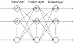
BP neural network is trained by a multi-level feedforward for the basic error back transmission method, which is represented as the popular used neural network. A BP neural network is typical of a forward network of the three or more levels with no feedback or no intra-level interconnect construction. The construction is shown in Figure 14. The transfer functions in BP neural networks usually are Sigmoid functions or linear functions. Its function expression is shown in formula (21):
| (21) |
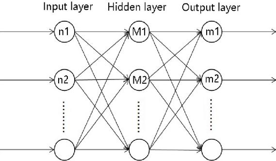
Figure 14 BP neural network structure.
According to the PCA analysis, it is determined that the first five meta-components include all the characteristic information of the fault data, then the number of input level nodes n is set to 5, and because this article has established four different fault states, the number of output level nodes m is set to 4. An amount of hidden layer nodes has a great impact on the property of BP network. The more hidden layer nodes amount, the stronger the learning ability of BP network. However, too many nodes will make the convergence slower. The fewer the number of nodes, the faster the convergence speed, but the network learning ability is very low, and the fault cannot be accurately identified. Then the number of hidden level nodes M can be expressed as:
| (22) |
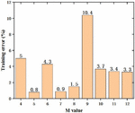
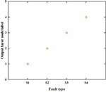
Since , and it is a constant, then the above values of and can be substituted into Equation (22), then the hidden level neuron node can be obtained. This article randomly selects a quarter of the 160 groups of samples collected in the experiment as training samples, in which only the value of parameter is changed. The training data is imported into the developed spatial model for training. Figure 15 indicates that when the value of is 5 and the result error is the least. Therefore, the hidden level nodes in BP neural network model can be chosen to be four. The prediction result of the impeller fault diagnosis system, as shown in Figure 16.
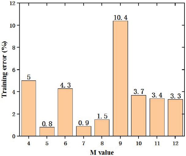
Figure 15 Training error with variables M.
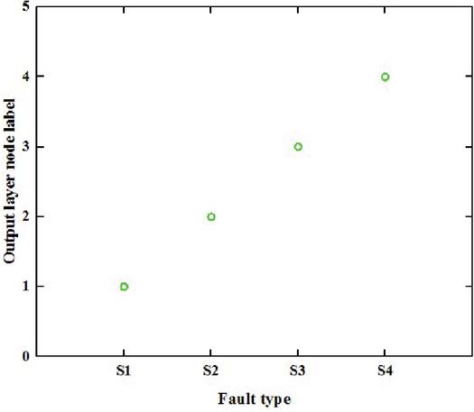
Figure 16 Predict the type of impeller failure.
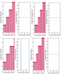
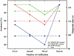
Quadruple cross-validation is usually used to verify the evaluation of models in the data. This method generally puts the signals into four sections, which is used for testing one group of data and training neural networks with three group of data. After noise elimination by the corresponding algorithm, the samples optimized by PCA are also divided into four parts, which are respectively introduced into BP neural network for quadruple cross verification. The results are shown in Figure 17. Accuracy is the average accuracy of multiple experiments, and the results are shown in Figure 18.
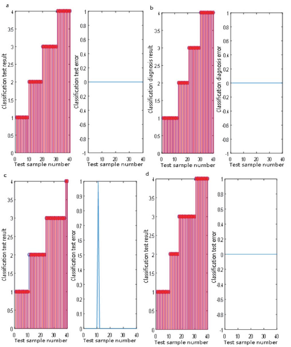
Figure 17 NPSO-PF-BP cross-validation diagram, a is the first verification, b is the second verification, c is the third verification, and d is the fourth verification.
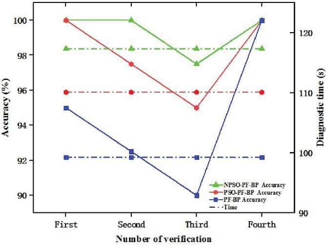
Figure 18 Comparison of diagnostic accuracy.
Figure 18 shows the diagnosis accuracy and diagnosis time of the three algorithms combined with BP neural network, and the diagnosis precision of the three diagnosis models is more than 90%. It explains the proposed diagnosis method for the detection of impeller fault state is effective and feasible. It is not difficult to see from the chart that the average diagnostic precision of NPSO-PF-BP model is the highest, followed by that of PSO-PF-BP model, and that of PF-BP model is the lowest. The results display the optimized PF method can further improve the diagnosis ability of mechanical structure state, and this paper put forward the NPSO-PF-BP algorithm has the best diagnosis capacity. The broken line of the dot line in the graph represents the corresponding algorithm diagnosis time. From the processing time of the whole diagnosis model, the NPSO-PF-BP model takes the shortest time, 9.8% faster than the PSO-PF-BP model and 15.4% faster than the PF-BP model. The results show that the NPSO-PF-BP diagnosis model can meet the requirements of real-time fault diagnosis with large and complex data.
To sum up, this article put forward the NPSO-PF-BP diagnosis method can effectively identify the four fault modes of centrifugal pump impellers established, and the diagnosis speed is the fastest and the diagnosis accuracy is the highest. At the same time, it also shows that the NPSO-PF-BP diagnosis method proposed in this paper is more suitable for mechanical fault diagnosis in complex environment.
5 Conclusion
In view of the increasingly sophisticated mechanized environment, the difficulty of fault diagnosis becomes higher, this article puts forward an optimized particle filter algorithm (NPSO-PF) suitable for noise elimination of non-linear systems by studying the basic theory of PF and PSO algorithms. The proposed diagnosis measure is used to the noise elimination processing of the spiral pump fault diagnosis study data of the four impeller status set up in this article. Finally, a centrifugal pump fault diagnosis way on the basis optimized particle filter (NPSO-PF)-BP). At the same time, for compare the effectiveness of the proposed diagnostic methods, PSO-PF-BP and PF-BP diagnostic models were set as control groups. The experimental results indicated that the NPSO-PF-BP centrifugal pump diagnostic method put forward in this article has the fastest diagnosis speed and the highest diagnostic precision, and is more suitable for mechanical fault diagnosis in current and future environments.
Acknowledgement
The Reliability Research Lab in the Department of Mechanical Engineering at the University of Alberta in Canada provided the original experimental data. The National Natural Science Foundation of China (Grant Nos. 51775390, 51901164, 51805378), the Natural Science Foundation of Hubei Province (Grant No. 2018CFB394), and the Foundation of Wuhan Science and Technology Bureau (Grant No. 2019010701011417) provides the financial support for paper research.
Conflict of Interest Statement
There are no conflicts to report about this paper.
References
[1] C. Lim, D. Kim, et al., The Operation Concept and Procedure of Mechanical Ground Support Equipment for KSLV-II Launch Complex, Journal of the Korean Society of Propulsion Engineers, 22(4), 2018, 125–132.
[2] Y.J. Li, Q.C. Chang, et al., Complex data study on mechanical fault diagnosing, Journal of Intelligent & Fuzzy Systems, 2018, 34(2), 1169–1176.
[3] Chen Hanxin, Fan Dongliang, Huang Jinmin, et al., Finite element analysis model on ultrasonic phased array technique for material defect time of flight diffraction detection, Science of advanced material 12(5) (2020), 665–675.
[4] Z.X. Li, S.J. Han, J.G. Wang, et al., Time-Delayed Feedback Tristable Stochastic Resonance Weak Fault Diagnosis Method and Its Application, Shock and Vibration, 2019, 2097164.
[5] Chen Hanxin, Huang Wenjian, Huang Jinmin, et al., Multi-fault condition monitoring of slurry pump with principle component analysis and sequential hypothesis test [J], International Journal of Pattern Recognition and Artificial Intelligence (2019), https://doi.org/10.1142/S0218001420590193.
[6] Z.P. Liu, L. Zhang, Naturally Damaged Wind Turbine Blade Bearing Fault Detection Using Novel Iterative Nonlinear Filter and Morphological Analysis, IEEE Transactions on Industrial Electronics, 2020, 67(10), 8713–8722.
[7] Hanxin Chen, Dong Liang Fan, Lu Fang, Wenjian Huang, Jinmin Huang, Chenghao Cao, Liu Yang, Yibin He and Li Zeng, Particle swarm optimization algorithm with mutation operator for particle filter noise reduction in mechanical fault diagnosis, International journal of pattern recognition and artificial intelligence (2020), https://doi.org/10.1142/S0218001420580124.
[8] X.C. Li, X.Y. Yang, Y.J. Yang, et al., An intelligent diagnostic and prognostic framework for large-scale rotating machinery in the presence of scarce failure data, Struct. Health Monit., 2020, 19(5), 1375–1390.
[9] A. Ul-Hamid, L.M. Al-Hadhrami, A.I. Mohammed, et al., Failure analysis of an impeller blade, Materials and Corrosion, 2015, 66(3), 286–295.
[10] Hanxin Chen et. al., Model-based method with nonlinear ultrasonic system identification for mechanical structural health assessment, Transactions on emerging telecommunications technologies (2020), e3955, http://doi.org/10.1002/ett.2955.
[11] P.K. Pradhan, S.K. Roy, A.R. Mohanty, Detection of Broken Impeller in Submersible Pump by Estimation of Rotational Frequency from Motor Current Signal, Journal of Vibration Engineering & Technologies, 2020, 8(4), 613–620.
[12] Q.C. Sun, B.W. Shi, et al., Fatigue Strength Evaluation for Remanufacturing Impeller of Centrifugal Compressor Based on Modified Grey Relational Model, Advances in Materials Science and Engineering, 2020, 1236130.
[13] W. Li, Y. Huang, A method for damage detection of a jacket platform under random wave excitations using cross correlation analysis and PCA-based method, Ocean Engineering, 2020, 214, 107734.
[14] F. Asghar, M. Talha, S.Y. Kim, et al., Hotelling T Index based PCA Method for Fault Detection in Transient State Processes, Journal of Institute of Control, Robotics and Systems, 2016, 22(4), 276–280.
[15] Cadini F, Sbarufatti C, Corbetta M, et al. Particle filtering-based adaptive training of neural networks for real-time structural damage diagnosis and prognosis [J]. Structural Control and Health Monitoring, 2019(11).
Biographies

Hanxin Chen obtained PHD in School of Mechanical and Aerospace Engineering at Nanyang Technological University in Singapore from July, 2001 to February, 2006. He was post-doc research fellow in Department of mechanical engineering at University of Alberta in Canada from March, 2006 to March, 2008. He was research associate in School of Physics at University of Windsor in Canada in 2012 and research scientist in Department of Control at Sheffield of University from December, 2012 to May, 2015. He is distinguished professor as “Chutian Scholar” of Hubei Province at Wuhan Institute of Technology from April, 2008. His research area is about condition monitoring and fault diagnosis of engineering system, structural health monitoring (SHM) etc.

Yuzhuo Miao is pursuing masters in School of Mechanical and Electrical Engineering at Wuhan Institute of Technology in China. His research interests are Structural Health Monitoring, fault diagnosis and nondestructive testing, etc.

Yongting Chen is student at Wuhan Britain-China School in China from Sept. 2019 to Jun. 2012. He joined the research project that is the National Natural Science Foundation of China (Grant No 51775390) as part-time research student in 2019.

Lu Fang graduated from Yangtze Normal University Normal University in 2017 and obtained master degree in School of Mechanical and Electrical Engineering at Wuhan University of technology in China in 2000. His research interests are Structural Health Monitoring, fault diagnosis, and non-destructive testing etc.

Li Zeng otained Ph.D in School of Materials physics and chemistry at Huazhong University of Science and Technology in China. She is Associate Professor in School of Mechanical and Electrical Engineering at Wuhan Institute of Technology in China. Her research interests are erosion-corrosion and protection of pipelines in oil and gas field.

Jun Shi is lecture at Wuhan Institute of Technology from 2017. His research area is reliability of the pipeline, simulation analysis by FEM, Design for higher pressure machine.
Journal of Web Engineering, Vol. 20_2, 253–280.
doi: 10.13052/jwe1540-9589.2022
© 2021 River Publishers