Generation of Realistic Navigation Paths for Web Site Testing Using RNN and GAN

Silvio Pavanetto^* and Marco Brambilla

Dipartimento di Elettronica, Informazione e Bioingegneria, Politecnico di Milano, Piazza Leonardo da Vinci 32, Milan, 20133, Italy
E-mail: silvio.pavanetto@polimi.it; marco.brambilla@polimi.it
*Corresponding Author

Received 29 October 2020; Accepted 20 October 2021; Publication 06 November 2021

Abstract

For applications that have not yet been launched, a reliable way for creating online navigation logs may be crucial, enabling developers to test their products as though they were being used by real users. This might lead to faster and lower-cost program testing and enhancement, especially in terms of usability and interaction. In this work we propose a method for using deep learning approaches such as recurrent neural networks (RNN) and generative adversarial neural networks (GANN) to produce high-quality weblogs. Eventually, we can utilize the created data for automated testing and improvement of Web sites prior to their release with the aid of model-driven development tools such as IFML Editor.

Keywords: Web engineering, deep learning, data mining, generative adversarial networks, recurrent neural networks, testing.

1 Introduction

Weblogs are representations of the navigation activity produced by a specified number of users on a certain website. This sort of data is critical, for example, for a corporation since it provides information about user behavior and how they interact with the firm’s product (website or application). The first valuable information that may be derived from a weblog is the website’s quality, as stated in Berendt and Spiliopoulou’s work [4] , where they attempt to comprehend navigation patterns that are present in the data. This is also addressed in Singh et al.’s study in 2013, [22], which provides an overview of web use mining strategies using pattern recognition. Furthermore, as shown in the work of Bernaschina et al. [5], one might evaluate these patterns and data regarding user actions using visualization tools.

If a company could have a realistic weblog before releasing its product, it would have a huge advantage since it could use the methods described above to observe the fewer visited web pages or those to place in the forefront, but it would need users and time to build them, making it a costly undertaking. Because of this constraint, our emphasis is on the generating aspect, which has received less attention, although it is a repeating topic in the research sector as well owing to a lack of publicly accessible data.

In reality, open source libraries such as Flog Generator [15] and Fake Apache Generator [3], as well as the work of Lin et al. [16], produce logs at random and cannot be utilized as datasets that reflect user behavior. As a result, being able to develop an algorithm that creates high-quality weblogs would be beneficial both scientifically and commercially.

We employed deep learning approaches to generate more realistic navigation activities, beginning with an RNN (Hochreiter Sepp and Jürgen Schmidhuber [13]), which has been shown to be capable of producing complicated sequences with long-range structure (Alex Graves et al. [12]). Then try a GAN (Goodfellow et al. 2014 [10]): neural networks that attempt to generate new data, such as pictures or text, that are highly close to the originals and often indistinguishable from them, and have grown in popularity in recent years.

The goal is to determine which technique for generating log data is the best and if the GAN is relevant to this situation. Our work begins with the development of a generative algorithm based only on ideas previously published in the literature on the analysis and production of weblogs. Then, we present two deep learning algorithms: an RNN and a GAN, and demonstrate their effective generating potential. Finally, we demonstrate how to utilize IFML Editor, a model-driven development tool, to describe and codify the structure of the legal URLs to be created.

This work is organized as follows: initially, we discuss the state of the art in web mining and discrete data sequences production. Then there is a section regarding the methodologies utilized in this study, which is followed by a section regarding implementation and experimentation. Finally, we conclude with conclusions and future work.

2 Related Work

Berendt and Spiliopoulou [4] proved the utility of the ”Web Usage Miner” (WUM) in 2000: a collection of tools that finds navigation patterns with sophisticated statistical and structural limitations. This effort sought to comprehend the quality, defined as the conformity of the web site’s structure to the intuition of each set of users visiting the site, of a given website as a whole, rather of viewing each page as a separate entity. They employed data mining methods such as sequence pattern mining and the apriori algorithm to do this.

Singh et al. [22] in 2013 provides an overview of the web use mining methodology by performing pattern recognition on weblog data, described as the process of taking in raw data and implementing an action based on the pattern’s ‘category.’ Their work is divided into three sections: pre-processing, pattern finding, and pattern analysis.

In general, these studies that analyze web log data for pattern identification employ almost the same method based on previously mentioned data pre-processing and data mining methods, with the addition of clusterization in certain situations (Vedaprakash et al. [23] and Mahoto et al. [17] are examples).

In terms of weblog data production, the open source malicious log detection package [generator-log-harmful-detection] attempts to produce fresh access log data by putting in certain malicious behaviors in order to identify them. The issue with [16] and other open source tools like Flog Generator [15] or Fake Apache Generator [3] is that these logs are generated at random. Instead, we make them in a totally different and more planned manner in this work. In terms of deep learning approaches used to generate discrete data, we begin with LSTM in recurrent neural networks (RNNs), which was initially introduced by Hochreiter Sepp and Jürgen Schmidhuber [13]. This form of RNN was extensively utilized in following publications, such as Alex Graves’ [12], which demonstrates how Long Short-term Memory recurrent neural networks can be used to construct complicated sequences with long-range structure by predicting one data point at a time. Their method is proven for text (with discrete data) and online handwriting (where the data are real-valued). Because of the effectiveness of this form of neural network when applied to data sequences (both real and discrete), this study suggests a Long Short-term Memory recurrent neural networks technique as the first deep learning technique.

In recent years, new strategies for generating high-quality data have been introduced; the most well-known and promising is the GAN (Goodfellow et al. 2014 [10]), which use a discriminative model to guide the training of the generative one. It does, however, have drawbacks when the purpose is to generate sequences of discrete tokens. One important problem is that the generator’s discontinuous outputs make it difficult to convey the gradient update from the discriminative model to the generative model. Furthermore, the discriminative model can only evaluate a whole sequence, however it is difficult to balance the present and future scores of a partly formed sequence after the whole sequence has been formed. Yu et al. [24] attempt to overcome this issue by developing SeqGAN, a sequence generating system. SeqGAN avoids the generator differentiation issue by directly executing gradient policy updating by modeling the data generator as a stochastic policy in reinforcement learning (RL). The RL reward signal is generated by the GAN discriminator and is sent back to the intermediate state-action stages through a Monte Carlo search. However, in their work, they employ a ’oracle’ model, that is a randomly initialized LSTM as the correct model, to create the true data distribution $p (x_{t} | x_{1}, \dots, x_{t - 1})$ for their experiments and assessments. They get a huge advantage in this way: it supplies the training dataset and then analyzes the precise performance of the generative models. In our technique, we utilize actual data as training data instead, and we assess the outcomes using several metrics at the conclusion of the GAN training.

3 Background

In this part, we provide an in-depth description of the backdrop required to support the job. The first section provides an overview of the data mining area, with a focus on the principles mentioned in the literature for the analysis of weblog data and the extraction of behavioral patterns. The emphasis of the second section of the chapter changes to the features of the kinds of algorithms that will be employed in the work for augmentation and production of the weblog data previously studied using data mining methods. First, we’ll go through the primary data mining methods that will be utilized for the baseline and to examine the dataset that will be utilized as input. The emphasis then moves to SVM (Support Vector Machines) [8] and how to utilize them to increase the algorithms’ performance. Finally, after providing a brief introduction of neural networks and the deep learning discipline, we will go into the theory of RNNs (Recurrent Neural Networks) [21] and GANNs (Generative Adversarial Neural Networks) [10].

3.1 Data Mining

Data mining is an interdisciplinary sub-field of computer science and statistics with the overarching objective of extracting information (through intelligent techniques) from a data collection and transforming the information into an intelligible structure for future use.

The true data mining job is to analyze vast amounts of data semi-automatically or automatically in order to identify previously undiscovered, intriguing patterns such as groupings of data records (cluster analysis), atypical records (anomaly identification), and relationships (association rule mining, sequential pattern mining).

3.1.1 Associations rules

Association rules are if-then statements that aid in demonstrating the likelihood of linkages between data items in huge data sets in many kinds of databases. Association rule mining offers a broad range of applications, including assisting in the discovery of sales correlations in transactional data or medical data sets.

Constraints on different metrics of relevance and interest are used to pick interesting rules from a collection of all feasible rules. The most well-known limitations are minimum support and confidence criteria.

Let $X$ represent an itemset, $X \Rightarrow Y$ represent an association rule, and $T$ represent a series of transactions from a specified database.

The amount of support indicates how often the itemset occurs in the dataset. The percentage of transactions $t$ in the dataset that includes the itemset $X$ is defined as the support of $X$ with regard to $T$ .

supp (X) = \frac{| {t \in T; X \subseteq t} |}{| T |}

The level of confidence indicates how often the rule has been shown to be correct. The confidence value of a rule, $X \Rightarrow Y$ , with relation to a collection of transactions $T$ is the percentage of transactions that include $X$ and also include $Y$ .

Confidence is defined as:

conf (X \Rightarrow Y) = supp (X \cup Y) / supp (X)

3.1.2 Apriori algorithm

Apriori is the most well-known algorithm for mining frequent itemsets and learning association rules in transactional databases. Agrawal and Srikant suggested it in a 1994 [2]. It then goes on to find the most often occurring individual items in the database and expands them to bigger and bigger item sets as long as those appear often enough in the database.

Apriori employs a “bottom-up” strategy in which frequent subsets are expanded one item at a time (a process known as candidate generation), and groups of candidates are evaluated against the data. When no further successful extensions are identified, the method finishes; it creates candidate itemsets of length $k$ from itemsets of length $k - 1$ . The candidates with an infrequent sub-pattern are then pruned.

3.2 Support Vector Machines

Support vector machines (SVMs, also known as support-vector machines) are supervised learning models with associated learning algorithms that examine data for classification and regression analysis in machine learning. Given a series of training examples, each of which is labeled as belonging to one of two categories, an SVM training method creates a model that assigns new instances to one of the two categories, resulting in a non-probabilistic binary linear classifier.

Intuitively, the hyperplane with the greatest distance to the closest training data point of any class (so-called functional margin) achieves a decent separation, since the greater the margin, the lower the classifier’s generalization error.

SVM are capable of non-linear classification in addition to linear classification due to the so-called “Kernel trick” [14], by locating a higher-dimensional space in which the original data points are linearly separable:

For a more detailed description of what a kernel is and what types of kernel exist, refer to [14].

3.3 Deep Learning

Machine-learning algorithms are used to recognize objects in photos, convert voice into text, match news articles, messages, or goods with the interests of users, and choose appropriate search results. Traditional machine-learning approaches were restricted in their capacity to interpret raw natural data.

Deep learning is a kind of machine learning technique that employs a cascade of numerous layers of nonlinear processing units for feature extraction and modification, with each subsequent layer using the output of the preceding layer as input. These algorithms acquire many layers of representations that correspond to distinct degrees of abstraction in supervised (e.g., classification) and/or unsupervised (e.g., pattern analysis) ways; the levels constitute a hierarchy of ideas.

3.3.1 Neural network

Artificial Neural Networks (ANNs) are a kind of computer model inspired by the way biological neural networks process information in the human brain.

The neuron, which is often referred to as a node or unit, is the fundamental computational unit of a neural network. It accepts input from other nodes or external sources and produces an output. Each input has a weight $w$ connected with it, which is determined by its relative relevance to other inputs, in addition to the input $1$ , which has a weight $b$ , which is the bias. The node applies a function $f$ , dubbed activation function, to the weighted sum of its inputs.

The activation function’s objective is to bring non-linearity into a neuron’s output; this is critical since the majority of real-world input is non-linear, and we want neurons to learn these non-linear representations. Depending on the kind of function, each activation function (or non-linearity) takes a single integer and performs a certain fixed mathematical operation on it.

When multiple neurons (nodes) are arranged in layers, nodes from adjacent layers are associated via connections or edges. All of these interactions have associated weights, and a feedforward process is present: information flows in a single direction – forward – from the input nodes, through any hidden nodes, and to the output nodes. The network contains no cycles or loops.

The technique through which a Multi-Layer Perceptron learns is referred to as Backpropagation, which was coined by [20]:

The total error is calculated at the output nodes and propagated back through the network using Backpropagation to determine the gradients, followed by an optimization approach such as Gradient Descent to alter the weights in the network with the goal of lowering the error at the output layer.

3.3.2 Recurrent neural network

A recurrent neural network (RNN) is a kind of artificial neural network (ANN) in which nodes form a directed graph along a succession of nodes. This enables it to demonstrate temporal dynamic behavior in response to a time sequence.

Unlike feedforward neural networks, RNNs can process sequences of inputs by using their internal state (memory). As a result, they may be used for tasks such as unstructured, connected handwriting recognition or voice recognition.

Unlike Feed-Forward Neural Networks map a single input to a single output, RNNs may map one to many, many to many (translation), or many to one (classifying a voice).

The Figure 1 depicts the information flow difference between an RNN and a Feed-Forward Neural Network.

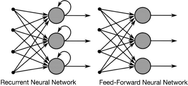
Figure 1 Feed-forwarding network vs Recurrent neural network.

There are two major obstacles RNN’s have to deal with:

• Exploding Gradients – when the algorithm places a high premium on certain weights for no apparent reason. This issue may be resolved by truncating or squashing the gradients.

• Vanishing Gradients – when the gradient values are too tiny and the model stops learning or takes an abnormally lengthy time to train as a result. This was a significant issue in the 1990s, and much more difficult to resolve than the expanding gradients. Sepp Hochreiter and Juergen Schmidhuber solved it using the LSTM idea [13].

LSTM (Long Short-Term Memory) Long Short-Term Memory (LSTM) networks are a kind of recurrent neural network that extends the memory of recurrent neural networks. As a result, it is highly adapted to learning from significant events separated by very lengthy time periods.

The units of an LSTM are utilized to construct the layers of an RNN, which is thus often referred to as an LSTM network. LSTMs allow RNNs to retain their inputs across time. This is because LSTMs store their data in a memory similar to that of a computer, since the LSTM can read, write, and erase data from its memory.

The issue of disappearing gradients is resolved by LSTM because it maintains sufficiently steep gradients, which keeps training time low and accuracy good.

3.3.3 Generative adversarial neural network

Generative Adversarial Networks (GANs) are a class of artificial intelligence algorithms used in unsupervised machine learning. They are implemented as a system of two neural networks competing in a situation in which each participant’s gain or loss of utility is precisely balanced by the loss or gain of utility of the other participant. If the participants’ total profits are brought together and their total losses are deducted, the total gains equals zero. They were first described in 2014 by Ian Goodfellow et al. [11].

The generative model is placed against an opponent in an adversarial networks framework: a discriminative model that learns to distinguish whether a sample is from the model distribution or the data distribution.

The competition in this game forces both sides to refine their techniques until the counterfeits are almost indistinguishable from the real. When both models are multilayer perceptrons, the adversarial modeling approach is the simplest to use. To ascertain the spread of the generator $p_{g}$ is specified as a prior on the input noise variables $p_{z} (z)$ , and then as a mapping to data space as $G (z; ϑ_{g})$ , where $G$ is a differentiable function represented by a multilayer perceptron with parameters $ϑ_{g}$ . Additionally, it is defined as a second multilayer perceptron $D (x; ϑ_{d})$ that produces a single scalar output. $D (x)$ denotes the likelihood that $x$ originated in the data rather than from $p_{g}$ . $D$ is trained with the goal of increasing the likelihood of correctly labeling both training examples and samples from $G$ . Simultaneously, $G$ is trained to minimize the value of $l o g (1 - D (G (z)))$ .

4 Model Driven Development for URLs Specification

To meet the objectives we set for ourselves in this work, including enhancing the structure of the site/app before release, we must establish a list of relevant URLs that reflect all potential pathways inside the completed product. There are many techniques for doing this, including extracting them from current logs (as we will do in the experiments) or compiling a list of potential URLs in preparation.

We chose Model-Driven Software Engineering (MDSE) or Model-Driven Engineering (MDE) strategies to attain the latter aim since various studies have proven how these methods may improve the efficiency and effectiveness of software development. In particular, we focus on the use case of Model-Driven Development (MDD), that proposes a streamlined process from requirement to implementation based on model design and proceeding through (semi)automated model transformations.

Given the complexity of developing comprehensive sets of correct navigational URLs, MDD can be beneficial as a guiding tool and strategy for generating the URLs of the respective UIs realizations. By using a modeling language for specyfying the interaction structure, we can derive rules to produce automatically the URLs of the respective web pages. In particular, we adopt the IFML language (Interaction Flow Modeling Language) [7], an international standard language defined by the Object Management Group (OMG) that can be used to visually specify in a platform-independent manner any graphical user interfaces. Through the language, developers can specify applications accessed or deployed on any platforms. IFML supports event-driven specification of the interactions and it integrates seamlessly with other languages for the specification of the business logic, including UML and BPMN. In particular, IFML focuses on the structure and behavior of the application front-end as perceived by the end user, thanks to the coverage of the following aspects: The view structure and components that define the contents visible in the UI; The events, which will be generated by the user’s interaction, application logic, or external agents and will affect the state of the UI; The reference to actions triggered by the user’s events; And the parameter binding between the elements of the UI. IFML is implemented and supported by various tools, including WebRatio¹ [1] and IFMLedit.org² [6], which provide modeling, validation, and code generation capabilities.

The main advantage of IFML is that it allows you to start from the visual model of the site / app and then thanks to the tools to generate the site itself and, always with MDD approaches, also the possible navigation URLs.

4.1 Generating URLs with IFML

We begin with an IFML representation of the application-to-be, construct high-level navigations inside the model, and potentially traverse its whole state space. This kind of study might be beneficial for assessments and testing throughout the design process. To take the study to the next level, we may investigate extending the study to include actual user behavior. Because user-like navigations are now available as produced URLs, it is simple to construct navigable URLs from our representation.

4.1.1 Modelling the system

To model the system, data is collected from JSON files generated by the online editor IFMLEdit.org and placed in a more convenient data format by deleting unnecessary information e.g. graphical layout connections. The representation maintains track of containers, components, events, and their confinement relationships, as well as any other information that may be associated with them. The destination container/component of the navigation, as well as any data bindings, are logged for events. Components include the collection, fields, and filters, as well as potential data bindings. Here are a few IFML model examples, together with the matching graphical representation of the given structure.

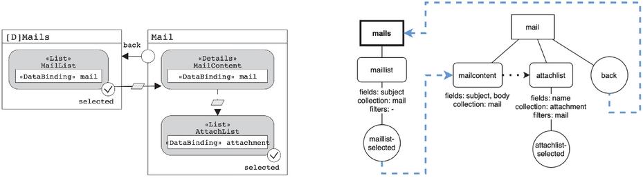
Figure 2 IFML Model and its graphical representation – Example 1.

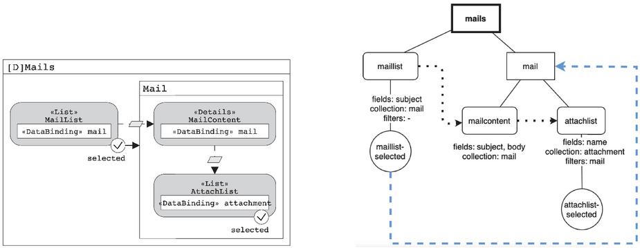
Figure 3 IFML Model and its graphical representation – Example 2.

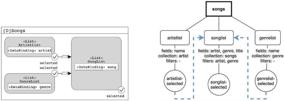
Figure 4 IFML Model and its graphical representation – Example 3.

4.1.2 Navigation paths specification

Navigations are formed from top level containers that are not contained in any other container. The events are then analyzed for each of them, beginning with those directly related to the considered container, progressing to those related to components, and eventually recursively analyzing each sub container.

In this study, only events that really lead to navigation are taken into account. A Navigation object is constructed from each of these, marking the objective of the navigation in terms of root container, that is, the one identifying the arrived page and, therefore, the one that will be required for producing the URL.

Finally, all data bindings from the event’s source root container are examined, retaining only those that constitute a relationship to a component in the destination container. Data bindings retain track of the target component (the one to which the value will be applied), the collection from which the binding’s value must be chosen, and, ultimately, filters that limit the possible options within a collection that are required to generate coherent future navigations.

Consider the previously mentioned example in Figure 4 and imagine that selecting a song from the song-list causes some navigation to another page that provides information about the chosen song. If the user lands on the page songs from the event artistlist-chosen, his song options will be limited to those of the chosen artist. Filters are useful for enforcing this kind of decision. Finally, duplication is avoided by maintaining a list of all created navigations and utilizing the existing reference in cases when numerous events trigger the same navigation. To be deemed equal, two navigations must go to the same container and have the same data bindings.

4.1.3 Generation of URLs

The last stage is to get from the abstract idea of navigation to a real URL. Data bindings are extracted by assigning a value taken from the provided collection to the appropriate component and, if necessary, meeting filter requirements. Finally, all components are combined to form the final string.

5 Deep Learning based Log Generation

This section describes our method for producing new weblogs. We began by creating a statistical strategy that would serve as our baseline. Following the first implementation, we created a recurrent neural network and a generative adversarial network (GAN) to generate fresh weblog data and compare the performances of all techniques.

5.1 Statistical Approach

The only public libraries we identified for producing logs do this process totally at random. This technique is so bad that we chose not to even consider it as a baseline. Instead, we offer a technique that is divided into two parts: the first analyzes a website and extracts statistical information, and the second utilizes that information to generate new weblogs. The input must include certain critical parts:

• Entry Points: A collection of pages that match to the navigation session’s entrance points. Each one is connected with a chance of starting the navigation with that page.

• Confidences: The confidences are the probability of shifting from one page to another at a given time. $T$ , knowing the whole navigation route taken from the start of the session (a chunk of continuous time in which the user is browsing without interruption or exiting the navigation.) until $T$ .

• Mean Times: A collection of typical times in seconds that relate to the amount of time people spend on a page on average.

• Web Site Graph: The graph depicting the whole web site, with each page connected with a list of potentially prior and subsequent pages.

The implementation employs cutting-edge technologies for extracting knowledge from logs and applying this data to the creation process. To generate new logs, we need to specify a few variables, such as the Maximum number of IPs at the same time, a List of user IPs, the Number of navigation sessions, and so on. Once all of the setup parameters have been specified, the algorithm begins the generation phase, in which the calculation of the Navigation Path is repeated for the number of navigation sessions previously defined. Each iteration is made up of the following steps:

• Selection of Entry Point: Every navigation session begins with the algorithm computing the entrance point of the series. This page is one of all the home pages that the algorithm has found to be picked by probability, with this page being picked by the algorithm in question. If a page is not included in the home pages list, it cannot be started in the navigation.

• Computation of Next URL: Following the selection of the entrance point, the algorithm selects the next URL in the sequence until the sequence length is reached: this is the exit condition of each loop iteration. This URL is chosen by getting all of the potential future pages for the previously calculated URL and then selecting one of them based on the likelihood of going from one page to the next.

• Computation of Residence Time: After selecting a couple of URLs, determine the amount of seconds the visitor will spend on page $A$ before going on to page $B$ or ending the navigation. This is accomplished by examining the Mean Times that are sent into the algorithm and selecting the mean time that corresponds to that couple of pages.

Once the loop cycle is finished and all of the sequences have been constructed, the algorithm generates a log file containing all of the previously produced user navigation activities. After sorting the requests by time, the file is generated. As previously shown, the first statistical method is driven by restrictions such as the probability of going from one page to another during each user’s journey and the residency duration on each page, which are already determined before the method begins its execution. Deep Learning approaches, on the other hand, do not need any human-designed feature extraction step since they provide the model with the potential of learning features optimized for the job at hand.

In Figures 5 and 6 the execution flow of the algorithm is shown. In particular, in Figure 5 the setting variable part and the sequences generation cycle are visible at a high level of abstraction. Instead, in Figure 6 the necessary steps for producing a single navigation session is shown.

Once the loop cycle is finished and all of the sequences have been formed, the algorithm generates a log file in the .txt or .log format that includes all of the previously produced user navigation activity. After sorting the requests by time, the file is generated.

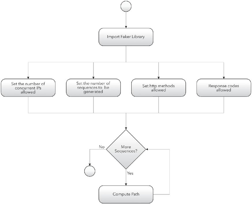
Figure 5 Execution flow of the weblog generation algorithm – baseline.

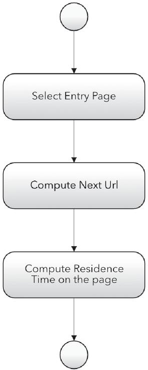
Figure 6 Execution flow of a single iteration of creating navigation sequence.

5.2 RNN-based Approach

We picked the Recurrent Neural Networks [20] (Rumelhart et al., 1986) among the deep learning methods because they are neural networks specialized to the processing of sequential input. When the temporal dependencies to be learnt are not too lengthy, simple RNNs are suitable. When this occurs, gradients propagated across several stages tend to evaporate (most of the time) or burst (more rarely). Even when we assume stable structures with a fair number of parameters, long-term dependencies result in exponentially lower weight updates for long-range interactions than for short-term interactions. As of now, the best answer to this issue has been discovered: gated RNNs, which are based on establishing pathways through time with derivatives that do not disappear or explode. Long Short-Term Memory (LSTM) is one of the most effective models that uses gated units [13].

We created an RNN that gets a list of navigation sessions as input and trains itself with them because of these qualities of Recurrent Neural Networks and their memory capacity. Following the training phase, the network is prepared to predict and generate new sequences.

In contrast to the statistical technique, we do not need to define the likelihood of switching between pages. As a result, the recurrent neural network’s input consists of a list of URL sequences, as well as the seconds of permanence on that page ( $s e c I n P a g e$ ) and the index that reflects the number of pages previously viewed in the same session ( $i n d e x S e s s i o n$ ). Each sequence corresponds to a single user’s navigation experience.

The major feature we want our RNN to learn is the sequence of pages that a certain user will view and the order in which he will go. As a result, we began by feeding the network merely the $u r l$ feature, then added the $s e c I n P a g e$ and $i n d e x S e s s i o n$ features. We arrive at the architecture shown in Figure 7, where we can observe that there are two main layers made of the CuDNNLSTM, which is accessible in the Keras framework.³

This form of LSTM cell can only be executed on GPUs and is based on Nvidia’s cuDNN. cuDNN implements common techniques such as forward and backward convolution, pooling, normalizing, and activation layers in finely tuned ways.⁴

Keras, a high-level neural networks API built in Python and capable of operating on top of TensorFlow, CNTK, or Theano, was utilized for the implementation.

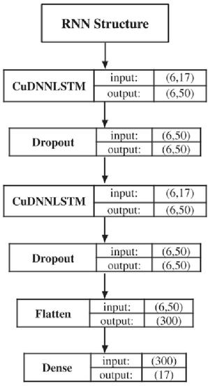
Figure 7 The RNN’s architecture. The following parameters are set: the length of each sequence is 6, the number of classes is 17, the number of neurons is 50, and the number of data points after the flatten operation is 300.

Each of these layers has 50 neurons and is followed by a dropout process to prevent overfitting. After the dropout, the output of the second layer is flattened to get a single 2D vector holding the inputs for the last layer: the Dense layer, which provides the network’s final output.

One thing that stands out in 7 is the presence of the number 6 across the network. Because the RNN’s definition is used on sequential data, this number relates to the length of every sequence of data that is supplied to the RNN, which implies data samples that vary over time.

In our instance, these changing samples are the navigation sessions, and it is critical for the network’s learning that each session matches exactly to a whole sequence that is processed. As a result, we decided to set a time limit for each navigation session.

In this manner, the RNN will be fed a whole session every time, and after $B$ sequences, where $B$ is the network’s batch size parameter, the batch of data will be processed through the network for each epoch.

Other concerns for the features and algorithm that comprise the RNN are as follows:

• Encoding of URLs: Because URLs are categorical in nature, they are encoded as categorical vectors of length $N$ , where $N$ is the total number of URLs contained in the dataset, and are comprised of 0s and 1s in the cell according to the value supplied by the $O n e H o t E n c o d e r$ function, which is provided in Sklearn.⁵ They are thrown out as output in this category shape in the network’s dense layer and then decoded in the original input form.

• Training phase: The RNN trains on the above-mentioned dataset using a K-fold cross validation procedure, in which the data is split into k subsets and one of the k subsets is used as the test set each time, while the other $k - 1$ subsets are combined to produce a training set. The overall efficacy of our approach is calculated by averaging the error estimates across all k trials. As a result, each data point appears precisely once in a validation set and $k - 1$ times in a training set. This considerably decreases bias since we are utilizing the majority of the data for fitting, and it also considerably decreases variance since the majority of the data is also used in the validation set. During this phase of training, the RNN will modify his weights per $B$ sequences it gets (where $B$ is the batch size defined as a hyper-parameter), iterating through the whole training set for $N$ epochs.

At the end of the training phase, the network is ready for predicting the next URL of a certain sequence and generating new ones. The test phase is done by checking the accuracy of the predictions with respect to the test set and the results will be discussed later in the evaluation section.

5.2.1 Adding SVM

After the initial RNN construction was completed and the accuracy of the predictions was determined, we reasoned that implementing a Support Vector Machine in the network’s final layer may boost prediction capabilities.

SVMs are strong regressors or classifiers that produce predictions based on a linear combination of kernel basis functions. As stated before in the background section, the kernel translates the input feature space to a higher dimensional space where the data is either linearly separable (in classification) or may be well fitted using a hyperplane (in regression).

Building a training set either by translating the sequential input into the frequency domain or by using constrained, fixed time windows of $m$ sequential input values is a limited means of applying current SVMs to time series prediction or classification. Such techniques, of course, are doomed to fail if temporal dependencies surpass $m$ steps.

SVM, for example, is unable to properly categorize all occurrences of the context-free language $a^{n} b^{n}$ ( $n$ a’s followed by $n$ b’s, for arbitrary integers $n > 0$ ). To address this limitation, we developed a recurrent SVM that solves the sequence learning challenge given in this paper using the RNN’s internal state representation.

To accomplish this purpose, we began with the formulation of the SVMs’ loss function, known as the Hinge Loss Function:

\max (0, 1 - y f (x))

(1)

where $f (x)$ is the SVM output given input $x$ and $y$ is the true class ( $-$ 1 or 1). The hinge loss is 0 when the true class is $-$ 1, for example. Figure 8 depicts a visual description.

We implemented the hinge loss function offered in Keras to the net’s last layer to apply this loss function in our RNN.

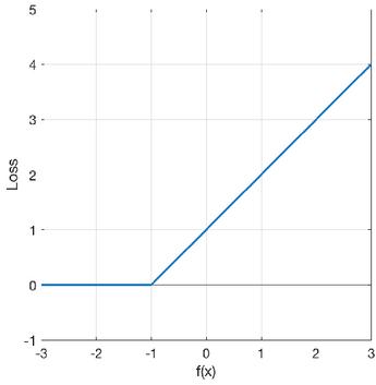
Figure 8 The representation of the hinge loss function of a SVM.

Setting the loss function to be identical to the SVM one is insufficient since Regularization is another essential parameter used in support vector machines. The regularization parameter (lambda) determines the relevance of miss-classifications.

SVM offer a quadratic optimization problem that seeks to maximize the margin between two classes while reducing miss-classifications. However, in order to develop a solution for non-separable situations, the miss-classification requirement must be eased.

As lambda becomes bigger, fewer incorrectly categorized instances are permitted. When lambda approaches infinity, the answer approaches the hard-margin (allow no miss-classification). The more miss-classifications are permitted when lambda approaches to 0 (but is not 0).

There is undoubtedly a trade-off between these two, and smaller lambdas, but not too tiny, are often employed to generalize effectively. The concept is comparable for non-linear-kernel SVM. Given this, greater values of lambda have a larger chance of overfitting, whereas lower values of lambda have a larger chance of underfitting.

To reproduce this behavior, we needed to add regularization to the RNN, which is why, in addition to the hinge loss function, a $l 2$ type of $k e r n e l_r e g u l a r i z e r$ from Keras’ regularizers was added to the network.

5.3 GAN-based Approach

Recurrent neural networks with long short-term memory (LSTM) cells have shown great performance in the job of creating sequential synthetic data that replicates the actual one, as detailed in the preceding section. To train an RNN, the most typical method is to maximize the log predictive probability of each valid token in the sequence given the previously observed tokens. The maximum likelihood techniques, on the other hand, suffer from exposure bias in the inference stage: the model builds a sequence repeatedly and predicts the next word based on previously predicted ones that may never be encountered in the training data. Such a disparity between training and inference might accumulate over time and become more noticeable as the duration of the sequence grows.

The Generative Adversarial Network (GAN) suggested by Goodfellow and colleagues [11] is a potential paradigm for addressing the aforementioned challenge. In GAN, a discriminative net $D$ learns if a given data instance is genuine or not, while a generative net $G$ learns to confound $D$ by producing high-quality data. This methodology has proven effective, however it has almost exclusively been used in computer vision applications involving the generation of samples of natural pictures (Denton et al. 2015 [9] is an example).

For these reasons, as well as his capacity to learn the probability distribution of training data and his hidden features, we believed that attempting to develop a GAN that creates synthetic discrete data would be an intriguing challenge and a worthwhile effort in determining if these types of Neural Networks are also adaptive to this job. Unfortunately, there are two issues with using GAN to generate sequences. To begin, GAN is intended to generate real-valued, continuous data but has difficulty immediately producing sequences of discrete tokens, such as messages or URLs in our situation.

As a result, the gradient of the loss from $D$ with respect to the $G$ outputs is used to lead the generative model $G$ (parameters) to slightly adjust the produced value to make it more realistic. If the produced data is based on discrete tokens, the discriminative net’s “slight modification” suggestion makes little sense since there is likely no comparable token in the small dictionary space.

Second, GAN can only deliver the score/loss for a full sequence after it has been formed; for a partly created sequence, balancing how good it is now and the future score as the complete sequence is difficult.

5.3.1 GAN parametrization

The input data for the construction of this net is a collection of URL sequences encoded as integers. Every sequence in this dataset, like the RNN input scenario, corresponds to a navigation session and has a defined length.

Looking more closely at the GAN’s implementation, the sequence generation issue is designated as follows:

Train a $θ -$ parameterized generative model $G_{θ}$ on a dataset of real-world structured sequences to build a sequence $Y_{1 : T} = (y_{1}, \dots, y_{t}, \dots, y_{T}), y_{t} \in Y$ , where $Y$ is the vocabulary of candidate URLs. This is seen as an issue of reinforcement learning. The state $s$ in timestep $t$ is the current created URLs $(y_{1}, \dots, y_{t} 1)$ , and the action a is the next URL $y_{t}$ to pick. Thus, the policy model $G_{θ} (y_{t} | Y_{1} : t - 1)$ is stochastic, but the state transition is deterministic once an action is taken, i.e. $δ_{s, s^{'}}^{a} = 1$ for the next state $s^{'} = Y_{1 : t}$ if the current state $s = Y_{1 : t - 1}$ and the action $a = y_{t}$ ; for other next states $s^{''}, δ_{s, s^{''}}^{a} = 0$ .

In addition, we train a $ϕ$ -parameterized discriminative model $D_{ϕ}$ to offer direction for enhancing the generator $G_{δ}$ . $D_{ϕ} (Y_{1 : T})$ is a probability indicating whether or not a sequence $Y_{1 : T}$ is derived from genuine sequence data. Positive examples from actual sequence data and negative examples from synthetic sequences created by the generative model $G_{θ}$ are used to train the discriminative model $D_{ϕ}$ . Simultaneously, the generative model $G_{θ}$ is updated using a policy gradient and MC search based on the predicted end reward from the discriminative model $D_{ϕ}$ . The reward is calculated based on the probability of fooling the discriminative model $D_{ϕ}$ .

Furthermore, as the generator advances, we must retrain the discriminator on a regular basis in order to stay up with it. Moreover, to decrease estimate variability, we employ distinct sets of negative samples coupled with positive data.

5.3.2 GAN structure

Finally, we’d like to provide some information regarding the two neural network structures that make up the GAN:

• Generator: The generative model we utilized was a recurrent neural network.

• Discriminator: In this situation, we chose CNN as our discriminator since these networks have shown remarkable success in text categorization, and our goal is quite similar to that. To generate a feature map, a kernel performs a convolutional operation on a window of words. At the conclusion of this step, the feature maps are subjected to a max-over-time pooling process. We employed a fully connected layer with sigmoid activation that outputs the likelihood that the input sequence is genuine to improve performance.

6 Evaluation

6.1 Context and Dataset

The assessment techniques and algorithms used in this study are based on the public NASA Apache web logs from 1995 [18]. This publicly accessible dataset is comprised of a regular Apache web log file. The Apache standard syntax for HTTP requests is a common setting for the access log, which also applies in this scenario. This common format may be generated by a wide variety of web servers and read by a wide variety of log analysis applications. The generated log file entries will look something like this (this is the usual apache format⁶): 127.0.0.1 – frank [10/Oct/2000:13:55:36 -0700] “GET/apache_pb.gif HTTP/1.0” 200 2326

This dataset was chosen for its size, quantity of entries, and because it is one of the few publicly accessible online log files: in fact, the lack of publicly accessible web log data is one of the concerns addressed in this study. The file is 205.2 MB in size and has 1891697 rows. It contains data from July 01 to July 31 (1995).

6.1.1 URL depth problem

One of the most crucial factors to handle is the depth of each URL that has to be retained for each request. That is, if we have a request with the following URL:

ltx_markedasmathitalic/home/shuttles/1969/apollo_11.html

We can see that the request link has four steps: home – shuttles – 1969 and apollo_11. Each step along this navigation route to the apollo_11.html page symbolizes a folder or, ultimately, a category of the website, progressing from the main page, which is the least particular page, to the shuttle “apollo11” page, which is the most particular page for that kind of shuttle. This is a standard conceptual depiction of pages on any website, but for the sake of this study, it symbolizes a problem whose complexity exponentially rises in specific conditions.

To illustrate this notion, it’s beneficial to look at the Table 1, which shows how quickly the number of unique pages on the website expands when the URL depth variable is increased. Indeed, we have just 19 distinct pages when just a portion of the URL is retained, but almost 10 times this amount with only one more depth level.

Table 1 The numbers of different pages with respect to the URL depth variable

URL Depth	Number of Pages
1	19
2	115
3	275
4	402

The issue with the algorithms we attempted to design is that each URL is treated as a category, and neural networks are tasked with predicting the next page in a series of all of them. This indicates that while the first instance (depth $=$ 1) requires networks to learn 19 distinct categories, the second instance (depth = 4) requires networks to learn 402 distinct categories, which is only possible with a massive quantity of training data, which is not accessible for our study.

6.1.2 Metrics

We used a statistic called the BLEU score [19] to assess the quality and realism of the logs generated by the various approaches. BLEU, or Bilingual Evaluation Understudy, is a score used to compare a candidate translation of text to one or more reference translations, or it is a method for assessing the quality of material that has been machine translated from one natural language to another. The correlation between a machine’s output and that of a person is referred to as quality.

Each URL is handled as a distinct “word” in the lexicon, consisting of all the pages of a single website. Individual translated segments – often phrases – are scored using this criterion by comparing them to a collection of high-quality reference translations. These ratings are then averaged over the whole corpus to determine the overall quality of the translation. In our example, the translated portions correlate to the created navigation sequences, whereas the high-quality reference translations relate to the NASA weblog.

6.2 Experiments With RNN

The network is implemented using Keras, a high-level neural network API developed in Python that can run on top of TensorFlow, CNTK, or Theano, while the LSTM cell type is CuDNNLSTM: This form of LSTM cell requires a GPU to execute and is based on Nvidia’s cuDNN. cuDNN implements typical procedures such as forward and backward convolution, pooling, normalizing, and activation layers with great precision.

To evaluate the network’s performance, we trained it on a training set and then tested the network’s prediction accuracy on a test set. The issue with this method of assessment is that we may meet URLs in the test data that were not observed during the training phase, and the findings will be inaccurate since the network cannot learn something it has never seen. As a result, we divided the data into training and test sets by ensuring that all URLs in the test set were also included in the training set. Additionally, we used many strategies to prevent overfitting, including dropout, early end training, and data shuffle.

The Table 2 contains the results of hyper-parameter tuning for a URL depth of one, while the Table 3 contains the evaluation results in terms of BLEU and highest accuracy for a URL depth of one.

As previously stated, the URL Depth issue is critical since it adds complexity to learning the proper features and degrades the network’s performance.

Table 2 RNN Experiments: Hyper-Parameters Tuning, URL Depth $=$ 1

*#test*	1	2	3	4	5
*Length Sequence*	6	6	6	6	6
*Neurons*	50	50	20	50	40
*Layers*	2	3	2	4	3
*Dropout*	0.2	0.25	0.25	0.25	0.2
*Shuffle*	True	True	True	True	True
*Batch Size*	30	30	30	20	40
*Activation*	softmax	softmax	softmax	softmax	softmax
*Optimizer*	adam	adam	adam	adam	adam
*Loss*	cat. cross-ent.	cat. cross-ent.	cat. cross-ent.	cat. cross-ent.	cat. cross-ent.
*Metrics*	accuracy	accuracy	accuracy	accuracy	accuracy
*Epochs*	50	50	65	70	100 (early stop)
*Average Accuracy*	74,13%	74,17%	74,69%	74,76%	74,76%

Table 3 RNN Experiments: BLEU performance and best accuracy with respect to the URL depth

URL Depth	#classes	BLEU	Best Accuracy
1	19	0.6482	74,76%
2	115	0.4739	58,23%
3	275	0.3655	31,05%

6.3 Experiments With GAN

The training set for the discriminator in this approach is made up of created examples labeled $0$ and cases from the training set labeled $1$ . To prevent overfitting, dropout and L2 regularization are utilized. Additionally, in this scenario, we attempted to create new sequences using three different URL depth levels in order to have a better understanding of how the GAN responds to this input.

The most critical parameters to adjust in this method are the number of training epochs for the generator and discriminator. Indeed, we observed that if the RNN (generator) is not appropriately trained before to beginning the adversarial training, the generator develops very slowly and unstable. The reason for this is because in this GAN, the discriminative model provides reward guidance during training, and if the generator acts almost randomly, the discriminator will identify the generated sequence as unreal with high confidence, and almost every action taken by the generator receives a low (unified) reward, which does not guide the generator in a positive improvement direction.

This suggests that significant pre-training is required before using adversarial training procedures to sequence generative models. To evaluate this technique, we began by analyzing the generator loss and correlating it to the URL depth and the number of generator pre-training epochs prior to adversarial training. We execute the training with three distinct pre-train generator epochs and three distinct URL Depth settings. The following conclusions are drawn from these analyses:

• By including a discriminator into the RNN, the GAN is able to reduce the generator’s loss and increase its limitations.

• When the URL Depth variable is increased, the loss value rises as well, independent of the generator pre-train epochs value. This is seen in the pictures 9 and provides more evidence that increasing the number of URLs is crucial for the complexity of the calculations that the network must do.

• In all situations, the variance of the loss reduces as the number of pre-train epochs grows. It is worth noting in the Table 4 that the lowest variance value occurs when the generator is pre-trained with 100 epochs, and this holds true for all three URL Depth levels. This translates into increased generator stability in comparison to scenarios with fewer pre-train epochs.

• When the depth is between 1 and 2, the minimum value of the loss is acquired after 15 pre-train epochs; when the depth is 3, the minimal value is acquired after 100 pre-train epochs. This indicates that the generator may achieve the lowest loss value with a small number of epochs, but the network will remain stable only with a large number of pre-train epochs.

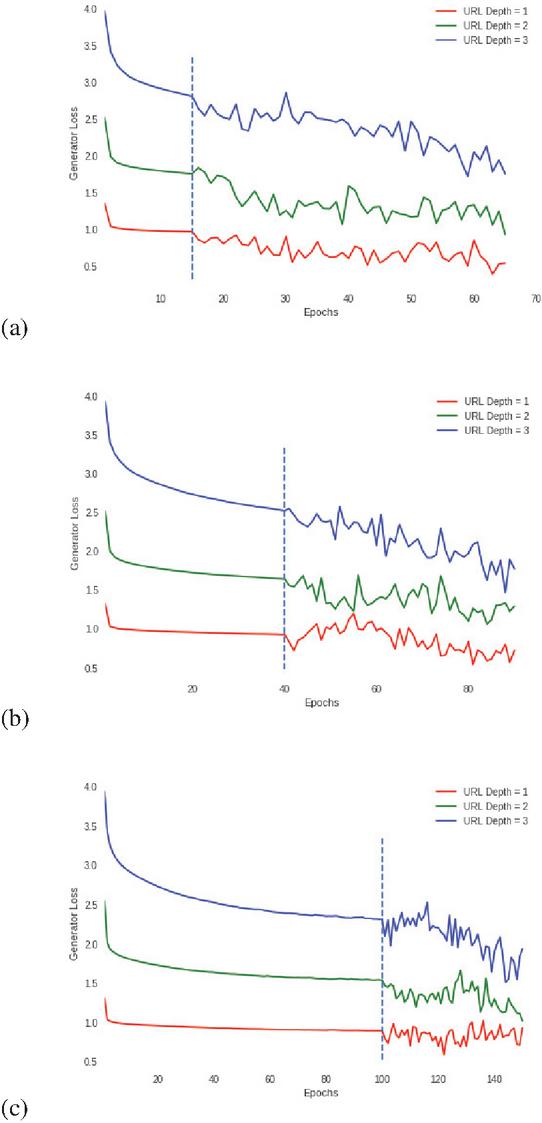
Figure 9 Generator loss with 15, 40, and 100 pre-training epochs respectively, in relation to different URL depth.

We constructed three distinct sets of sequences based on the URL depth and the number of pre-train epochs used by the generator, and compared the BLEU score to the original set of sequences. The findings are tabulated in 6. As can be seen, adding a discriminator to the RNN (the generator) increases the scores in each of the three scenarios but only if the generator has a sufficient number of pre-train epochs. If we train the generator for just 40 epochs and then begin adversarial training, the discriminator will always reward the data created by the RNN with a low score.

This is in contrast to prior evaluations, in which we demonstrated that the lowest loss values are obtained with 15 or 40 pre-train epochs, but agrees on the fact that network stability is increased with 100 pre-train epochs. This illustrates that when it comes to generative models, analyzing pure loss alone is insufficient to determine if these models generate high-quality data.

Table 4 GAN Experiments: Variance of the generator loss, related to the URL Depth and the pre-train epochs

	URL Depth $=$ 1	URL Depth $=$ 2	URL Depth $=$ 3
15 Epochs	0.0151	0.0324	0.0673
40 Epochs	0.0255	0.0239	0.0614
100 Epochs	0.00832	0.0179	0.0550

Table 5 GAN Experiments: Variance in generator loss as a function of URL Depth and pre-train epochs

	URL Depth $=$ 1	URL Depth $=$ 2	URL Depth $=$ 3
15 Epochs	0.3916	0.9308	1.7240
40 Epochs	0.5451	1.0667	1.4720
100 Epochs	0.5922	1.0215	1.5121

Table 6 GAN Experiments: BLEU performance with respect to the URL depth

URL Depth	BLEU, 40 Pre-train Epochs	BLEU, 100 Pre-train Epochs
1	0.6071	0.7243
2	0.4328	0.5471
3	0.3321	0.4839

7 Comparison: Statistical Approach vs RNN vs GAN

For the final comparison of all the algorithms examined in this study, we chose to utilize a measure other than BLEU, namely human judgment, since a weblog is composed of navigation sequences, each of which is determined and generated by a person. As a result, we picked five of our colleagues with similar abilities and expertise and showed them all the website’s pages and various navigation pathways. We blend 50 genuine sequences with 50 produced using GAN and RNN.

The judges are then asked to determine whether each of the 100 sequences was generated by humans or computers. Once determined to be genuine, it receives a score of $+$ 1; otherwise, it receives a score of 0. Finally, an average score is generated for each algorithm. The experiment findings are summarized in Table 7, demonstrating the considerable advantage of GAN over RNN and statistical methods for weblog production.

8 Conclusions and Future Work

We suggested a method for automatically producing high-quality weblogs using deep learning methods such as recurrent neural networks and generative adversarial neural networks in this study. We conducted a state-of-the-art investigation with the goal of identifying ways for reproducing and improving the greatest performance achieved today using generative algorithms for discrete sequences of data.

Table 7 Weblog generation performance comparison

Algorithm	Statistical	RNN	GAN
Human Score	0.4335	0.5400	0.6450
BLEU	0.5811	0.6482	0.7243

We began by implementing a state-of-the-art algorithm that improves random approach performance by mining data and constructing navigation sequences based on association criteria. Then, we constructed a recurrent neural network that attempts to learn the probability distribution of the input data and is capable of predicting the correct URLs to finish a given incomplete sequence with reasonable accuracy when the number of features is small, but is not resilient when the number of features is huge.

Finally, we constructed the GAN by using a convolutional neural network as the discriminator, allowing the RNN to self-improve through a so-called min-max game between the two networks. Our findings validate the idea that generative adversarial neural networks are the optimal family of models for weblog creation, outperforming recurrent models in particular when the number of feature variables is significantly increased. We demonstrated that when the generator is sufficiently trained, the GAN outperforms the RNN and statistical method using both the BLEU and Human metrics. Rather than that, whether the generator’s pre-train epochs are insufficient or excessive, the quality of the produced sequences is lower than that of RNN but still greater than that of statistical sequences.

8.1 Future Work

Along with the option of introducing additional variables in the network’s training phase to enhance the quality of the produced weblog, we discussed the work provided by [5] for displaying weblog data on a graphical representation of a specific website or app using a model-driven tool (IFMLEdit). In addition, we have shown a formalization of the links generated through this tool.

With the GAN, future work might include the generation of new weblogs and feeding them into the website’s model. Then, two models might be compared, one fed with human-generated logs and the other using GAN logs.

Acknowledgements

This research has been partially funded by the Spanish government under the project LOCOSS, PID2020-114615RB-I00/AEI/10.13039/501100011033.

References

[1] Roberto Acerbis, Aldo Bongio, Marco Brambilla, and Stefano Butti. Model-driven development based on omg’s IFML with webratio web and mobile platform. In Engineering the Web in the Big Data Era – 15th International Conference, ICWE Proceedings, pages 605–608, 2015.

[2] Rakesh Agrawal and Ramakrishnan Srikant. Fast algorithms for mining association rules in large databases. In Proceedings of the 20th International Conference on Very Large Data Bases, VLDB ’94, pages 487–499, San Francisco, CA, USA, 1994. Morgan Kaufmann Publishers Inc.

[3] Kirit Basu. Fake apache log generator, 2015–2018.

[4] Bettina Berendt and Myra Spiliopoulou. Analysis of navigation behaviour in web sites integrating multiple information systems. The VLDB Journal—The International Journal on Very Large Data Bases, 9(1):56–75, 2000.

[5] Carlo Bernaschina, Marco Brambilla, Thanas Koka, Andrea Mauri, and Eric Umuhoza. Integrating modeling languages and web logs for enhanced user behavior analytics. In Proceedings of the 26th International Conference on World Wide Web Companion, pages 171–175. International World Wide Web Conferences Steering Committee, 2017.

[6] Carlo Bernaschina, Sara Comai, and Piero Fraternali. Ifmledit.org: model driven rapid prototyping of mobile apps. In Proceedings of the 4th International Conference on Mobile Software Engineering and Systems, pages 207–208. IEEE Press, 2017.

[7] Marco Brambilla and Piero Fraternali. Interaction Flow Modeling Language: Model-Driven UI Engineering of Web and Mobile Apps with IFML. Morgan Kaufmann Publishers Inc., San Francisco, CA, USA, 2014.

[8] Corinna Cortes and Vladimir Vapnik. Support-vector networks. Machine Learning, 20(3):273–297, Sep 1995.

[9] Emily L Denton, Soumith Chintala, Rob Fergus, et al. Deep generative image models using a laplacian pyramid of adversarial networks. In Advances in neural information processing systems, pages 1486–1494, 2015.

[10] Ian Goodfellow, Jean Pouget-Abadie, Mehdi Mirza, Bing Xu, David Warde-Farley, Sherjil Ozair, Aaron Courville, and Yoshua Bengio. Generative adversarial nets. In Z. Ghahramani, M. Welling, C. Cortes, N. D. Lawrence, and K. Q. Weinberger, editors, Advances in Neural Information Processing Systems 27, pages 2672–2680. Curran Associates, Inc., 2014.

[11] Ian Goodfellow, Jean Pouget-Abadie, Mehdi Mirza, Bing Xu, David Warde-Farley, Sherjil Ozair, Aaron Courville, and Yoshua Bengio. Generative adversarial nets. In Advances in neural information processing systems, pages 2672–2680, 2014.

[12] Alex Graves. Generating sequences with recurrent neural networks. arXiv preprint arXiv:1308.0850, 2013.

[13] Sepp Hochreiter and Jürgen Schmidhuber. Long short-term memory. Neural computation, 9:1735–80, 12 1997.

[14] Martin Hofmann. Support vector machines—kernels and the kernel trick. Notes, 26, 2006.

[15] MinJae Kwon. Flog, an apache log generator, 2017–2018.

[16] Chu-Hsing Lin, Jung-Chun Liu, and Ching-Ru Chen. Access log generator for analyzing malicious website browsing behaviors. In 2009 Fifth International Conference on Information Assurance and Security, pages 126–129. IEEE, 2009.

[17] NA Mahoto, A Memon, and MA TEEVNO. Extraction of web navigation patterns by means of sequential pattern mining. Sindh University Research Journal-SURJ (Science Series), 48(1), 2016.

[18] NASA. Nasa apache web log, 1995.

[19] Kishore Papineni, Salim Roukos, Todd Ward, and Wei-Jing Zhu. Bleu: A method for automatic evaluation of machine translation. In Proceedings of the 40th Annual Meeting on Association for Computational Linguistics, ACL ’02, pages 311–318, Stroudsburg, PA, USA, 2002. Association for Computational Linguistics.

[20] David E Rumelhart, Geoffrey E Hinton, and Ronald J Williams. Learning representations by back-propagating errors. nature, 323(6088):533, 1986.

[21] Alex Sherstinsky. Fundamentals of recurrent neural network (RNN) and long short-term memory (LSTM) network. CoRR, abs/1808.03314, 2018.

[22] Nanhay Singh, Achin Jain, and Ram Shringar Raw. Comparison analysis of web usage mining using pattern recognition techniques. International Journal of Data Mining & Knowledge Management Process (IJDKP) Vol, 3:137–147, 2013.

[23] Mr PG Vedaprakash, Mr PG Om Prakash, and Mr M Navaneethakrishnan. Analyzing the user navigation pattern from weblogs using data pre-processing technique. International Journal of Computer Science and Mobile Computing, ISSN, pages 90–99, 2016.

[24] Lantao Yu, Weinan Zhang, Jun Wang, and Yong Yu. Seqgan: Sequence generative adversarial nets with policy gradient. In Thirty-First AAAI Conference on Artificial Intelligence, 2017.

Biographies

Silvio Pavanetto is a research fellow at Politecnico di Milano. His research interests include data science, social media monitoring, data-driven innovation, and big data analysis with particular attention to machine learning and deep learning techniques, applied on different scenarios and types of data, such as time series, images and text. In his two years of research he was the author of several papers published in international conferences and he worked on several research projects, also in collaboration with other European universities.

Marco Brambilla is a full professor at Politecnico di Milano. He manages several research projects and industrial innovation activities. His research interests include data science, software modeling languages, crowdsourcing, social media monitoring, data-driven innovation, and big data analysis. He has been visiting researcher at CISCO and UCSD, USA, and visiting professor at Dauphine University, Paris. He is the main author of the OMG standard IFML. He founded 3 startups and authored over 250 papers, 2 patents, and 5 books. He is editor and associate editor of various journals and he has been PC Chair of two editions of the ICWE Web Engineering Conference.