A Probability Distribution and Location-aware ResNet Approach for QoS Prediction
Wenyan Zhang, Ling Xu*, Meng Yan, Ziliang Wang and Chunlei Fu
School of Big Data & Software Engineering, ChongQing University, Chongqing, 400044, China
E-mail: xuling@cqu.edu.cn
*Corresponding Author
Received 12 November 2020; Accepted 27 May 2021; Publication 25 June 2021
Abstract
In recent years, the number of online services has grown rapidly, invoking the required services through the cloud platform has become the primary trend. How to help users choose and recommend high-quality services among huge amounts of unused services has become a hot issue in research. Among the existing QoS prediction methods, the collaborative filtering (CF) method can only learn low-dimensional linear characteristics, and its effect is limited by sparse data. Although existing deep learning methods could capture high-dimensional nonlinear features better, most of them only use the single feature of identity, and the problem of network deepening gradient disappearance is serious, so the effect of QoS prediction is unsatisfactory. To address these problems, we propose an advanced probability distribution and location-aware ResNet approach for QoS Prediction (PLRes). This approach considers the historical invocations probability distribution and location characteristics of users and services, and first uses the ResNet in QoS prediction to reuses the features, which alleviates the problems of gradient disappearance and model degradation. A series of experiments are conducted on a real-world web service dataset WS-DREAM. At the density of 5%–30%, the experimental results on both QoS attribute response time and throughput indicate that PLRes performs better than the existing five state-of-the-art QoS prediction approaches.
Keywords: QoS prediction, deep learning, ResNet, probability distribution.
1 Introduction
With the rise of various cloud application platforms, the number of various services increases rapidly. At the same time, users are more likely to invoke the services of these cloud platforms to implement relevant functions instead of downloading various applications. However, there are many candidate services in the cloud environment, which makes it difficult for users to choose a suitable service. So researchers are trying to find some ways to help users find better services among many with the same functionality.
Quality of service (QoS) is the non-functional evaluation standard of service, including service availability, response time, throughput, etc. Its value is often affected by the network environment of the user and the service. In different network environments, QoS values generated by different users may vary greatly even if the invoked service is the same one. Therefore, it is meaningful to predict QoS values of candidate services before the user invokes a service, which can help the target user distinguish the most suitable service among different functionally equivalent services according to the predicted QoS results [2, 9, 8, 33, 7, 31]. At present, QoS value has become a pivotal criterion for service selection and service recommendation, and QoS prediction has also been applied in plenty of service recommendation systems.
In recent years, collaborative filtering(CF) methods are widely used for QoS prediction [39, 38, 28, 24, 3, 19, 22], which relies on the characteristics of similar users or items for target prediction. In QoS prediction, the collaborative filtering methods match similar users or services for target users or services first, and then uses the historical invocations of these similar users or services to calculate the missing QoS. Because of its strong pertinence to the target user and item, CF is often used in personalized recommendation systems. However, CF can only learn low-dimensional linear features, and its performance is usually poor in the case of sparse data. To address these problems, several QoS prediction approaches based on deep learning have been proposed, and these approaches have been proved to be very effective in QoS prediction [33, 32, 36, 30]. Yin et al. [33] combined Matrix Factorization (MF) and CNN to learn the deep latent features of neighbor users and services. Zhang et al. [36] used multilayer-perceptron (MLP) capture the nonlinear and high-dimensional characteristics. Although the existing deep learning methods have improved in QoS prediction, they will not perform better when the network is deep due to the inherent gradient disappearance of deep learning. Inspired by the deep residual learning(ResNet) [10], which is widely used in the field of image recognition, we realize that the reuse feature can effectively alleviate the gradient disappearance problem in deep learning. ResNet consists of multiple residual blocks, each of which contains multiple shortcuts. These shortcuts connect two convolution layers to realize feature reuse, prevent the weakening of original features of data during training, and achieve the purpose of alleviating gradient descent.
Among the existing deep learning approaches, most of them [33, 32] only use ID as the characters, and a few methods [36] introduce the location information. However, users and services in the same region often have similar network status, which provides a crucial bases for finding similar neighborhoods. Therefore, the introduction of geographic position is often helpful for achieving higher accuracy in QoS prediction. In addition, none of these methods consider using probability distribution as the characteristic. Probability distribution refers to the probability of QoS predictive value in each interval, which is calculated by the historical invocations of the target. For example, if a user’s invocation history indicates that the response time is almost always less than , the probability of missing value less than is much higher than the probability of missing value greater than 0.5s. Therefore, the introduction of probability distribution could reflect the historical invocation of users and services. For QoS prediction, historical invocation is the most important reference basis, so it is necessary to introduce probability distribution as a feature in QoS prediction.
Therefore, in this paper, we propose a probability distribution and location-aware ResNet approach(PLRes) to better QoS prediction. First, PLRes obtains the information of target users and services, including identifier information, geographical location and historical invocation, and calculates the probability distribution of target users and services according to the historical invocation. Then PLRes embedded ID and location characteristics into high-dimensional space, and concatenated the embedded feature vectors and probability distribution vectors. Next, the ResNet is used to learn the nonlinear feature of the combined characteristics. Finally, PLRes is exploited to predict the missing QoS value.
The contributions of this paper are as follows:
• We calculate the probability distribution of target users and services and take them as the characteristics of QoS prediction. This characteristic reflects the network conditions of target users and services, and reduces the error of Qos prediction.
• We propose a novel probability distribution and location-aware QoS prediction approach PLRes, which is based on ResNet. In our approach, we use the identifier, location information and probability distribution as the characteristics, and first introduce the ResNet for QoS prediction, which uses the idea of feature reuse to enhance the features in the process of model training. This enables our model to learn nonlinear high-dimensional characteristics well and get better results when the network depth increases.
• We validated the PLRes on a real-world dataset, WS-DREAM1, and compared the predictive performance with various existing classical QoS prediction methods and the state-of-the-art deep learning approach LDCF [36]. Experimental results show that our method outperforms the state-of-the-art approach for QoS prediction significantly.
The remainder of the paper is organized as follows. In Section 2, we provide some background of our research. In Section 3, we describe our QoS prediction model in detail. In Section 4, we introduce the experiment setup, followed by experimental results and discussion in Section 5. In Section 6, we provide an overview of related works. In the last section, we conclude our work and provide an outlook on directions for future work.
2 Preliminaries
In this section, we will make a brief introduction to the knowledge related to the research.
2.1 QoS Matrix
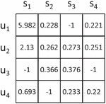
QoS is the quality of service, including static attributes and dynamic attributes. Static attributes are those whose values do not change, such as the cost; dynamic attributes are those whose values always change, including response time, throughput, etc. Static properties are fixed values provided by the service provider and can be used directly for service filtering conditions. However, dynamic attributes change at any time, and different users may get very different QoS values even if the service they invoke is the same one. The construction of the QoS matrix and the prediction of QoS both aim at these dynamic attributes. User and service are taken as the dimensions to describe the QoS value respectively, and the obtained matrix is the QoS matrix. Take response time as the example, the form of the QoS matrix is shown in the Figure 1, -1 represents the invalid response time, which means the user did not invoke the service or the response time timeout for invoking the service. For user in Figure 1, user has not effectively invoked service , while the response time of invoking service , and is , and , respectively.
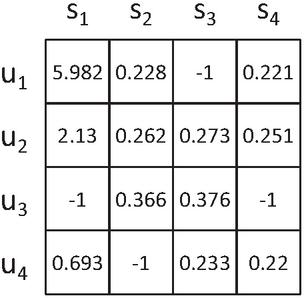
Figure 1 QoS matrix(taking response time as an example).
Density is usually used to represent the valid value ratio of the QoS matrix. In Figure 1, the matrix should contain 16 QoS values, among which 12 are valid, so the density of the matrix is 75%. However, in the real world, the number of services invoked by each user is strictly limited, which results in very few accurate QoS values that can be obtained, which means that the QoS matrix is very sparse. In order to simulate the real situation, the matrix density is usually controlled below 30% in related studies.
2.2 QoS Distribution
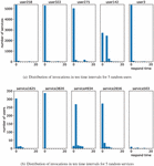
QoS distribution is the distribution of QoS in different value ranges. The distribution of QoS values of different users and services are often different. Taking response time as an example, we randomly select users and services from the real-world dataset and calculate their historical QoS distribution.

Figure 2 Distribution of invocations random samples.
A record with a response time of more than is assumed to be an invalid record with a response timeout, and takes less than as the valid QoS values. Suppose we set the number of intervals to 10, then each interval spans 2 seconds. Figure 2(a) shows the distribution of historical invocation for five different users, and Figure 2(b) is the distribution for the services. The abscissa axis represents the time interval and the ordinate axis represents the number of invocations. More specifically, the Y-axis of Figure 2(a) is the number of services invoked by the target user, and the Y-axis of Figure 2(b) is the number of users that invoked the target service. Take the in Figure 2(a) as an example, there are 5366 services whose response time is less than , 92 services whose response time is greater than and less than , and so on until . As can be seen from the Figure 2(a), the service response time distribution of several users is mainly concentrated within , but the distribution of is quite different. In fact, we also randomly checked the QoS distribution of some other users, most of which were similar to and , while the distribution of a small number of users was quite different from that of other users. The historical distribution of services also shows a similar pattern: the response times of most services are similar to those of , , and in Figure 2(b), while a few services are abnormal, such as and .
Therefore, QoS distribution is helpful in reflecting sample characteristics. Considering the total number of historical invocations by different users or services are always different, the distribution proportion of QoS is usually taken as the probability distribution of QoS, so the calculation method is as follows:
| (1) | ||
| (2) |
where , denotes the probability of the QoS appearing in th interval according to the historical invocations of user and service ; , denotes the number of the QoS appearing in th interval according to the historical invocations of user and service ; , denotes the total number of the user ’s invocations and the service ’s respectively. Take the first user in Figure 2(a), as an example, the QoS used by this distribution is response time, with set to 10. Since the dataset used records the maximum response time as 20s, it is set to an interval every 2 seconds. The number of invocation records by in each interval is [5366, 92, 22, 5, 8, 15, 33, 4, 2, 2], and the total number is 5549. So the in 10 interval probability is [96.7%, 1.66%, 0.4%, 0.09%, 0.14%, 0.27%, 0.59%, 0.07%, 0.04%, 0.04%].
2.3 Residual Network
The increase of network depth is often helpful to improve network performance. The reason is that the rise of network parameters makes the network acquire a stronger nonlinear expression ability to fit more complex characteristic inputs. However, conventional network stacking is often accompanied by gradient vanishing/explosion problems, which seriously hinders the convergence of the model. In 2015, He et al. [10] proposed the residual network(ResNet), which effectively alleviated the problem of gradient disappearance in deep learning networks and was widely used in image recognition technology.
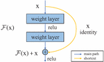
The residual network consists of several residual blocks. The residual block equivalently maps the output of the previous layer and passes it to the next layer by shortcut connection, which is also the design idea of the residual network. As shown in Figure 3, a residual block consists of a main road and a shortcut. The main path is the original stack network, and the input x is mapped through (x); In the shortcut, do the equivalent mapping to x.

Figure 3 Residual learning: a building block.
Assuming the final mapping is (x), the mapping in the main path (x):=(x)-x, and the original mapping is recast as (x)+x. What the network learns is not the (x) of the complete output, but the difference between the output and the input (x)-x, that is, the residual. By using shortcuts in the original stack network, the problem of gradient descent approximating to 0 caused by the multiplication of weight coefficients less than one is avoided. The reuse of original features is realized, and gradient disappearance in the network training is alleviated.
3 Proposed Approach
In this section, we give a detailed description of the proposed approach.
3.1 The Framework of the Proposed Model
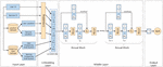
The overall architecture of PLRes is shown in Figure 4, which includes the input layer, the embedding layer, the middle layer, and the output layer.
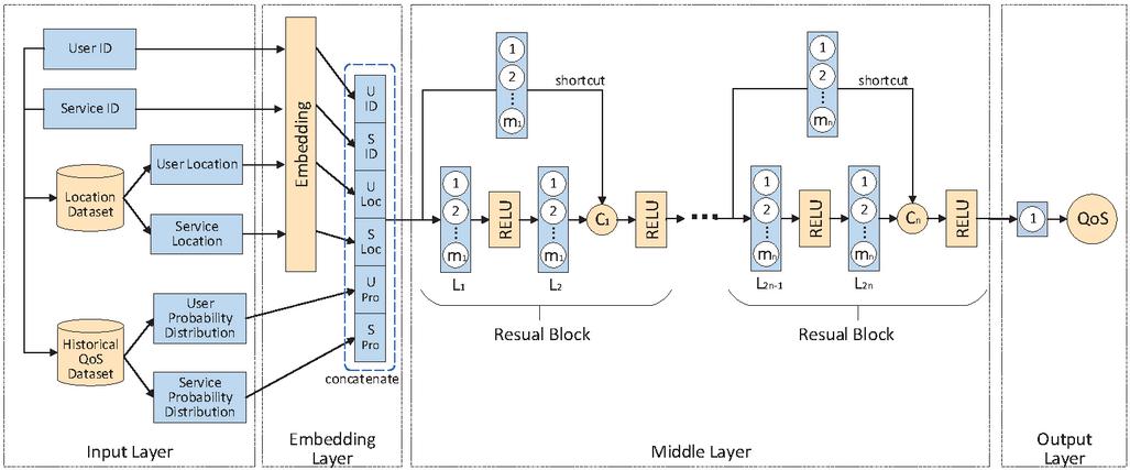
Figure 4 The framework of the proposed model.
The process of PLRes can be expressed as: the model receives a pair of user and service characteristics(including ID, location and probability distribution) as input, then embedded the identity and location features in the high-dimensional space respectively. Next, the embedded vectors and the probability distribution are concatenated into a one-dimensional vector. PLRes learns the one-dimensional feature and finally, gives the prediction result according to the learned characteristic rule. The following subsections describe the model details. Section 3.2 and 3.3 describe the input and embedding of features respectively. Section 3.4 describes the learning process of the model. Section 3.5 describes the final prediction and output details, and Section 3.6 describes the setting of the model optimizer and loss function.
3.2 Input Layer
The input layer is primarily responsible for receiving features. The features we selected include the user ID, the user’s location, the user’s probability distribution, the service ID, the service’s location and the service’s probability distribution. Both the user ID and the service ID are represented by an assigned integer. So only one neuron is needed for the input of both. The location information of the user and the service is represented by country and AS(Autonomous System), so the location information of the user and the service each needs two neurons. The probability distribution needs to be calculated based on historical invocations. The calculation is carried out in Section 2.2. At the input layer, the corresponding probability distribution of the target user and target service is obtained through the user ID and service ID as the probability feature. The number of neurons required in the input layer is related to the number of the QoS value interval .
3.3 Embedding Layer
The embedding layer mainly does two jobs: embedding ID and location features into the high-dimensional space, and feature fusion for all features. At first, it maps the discrete features into high-dimensional vectors. There is no doubt that in our dataset, ID, country and AS are all discrete features, which need to be encoded to be the data that deep network computing can be used.
In the embedding layer, we use one-hot to encode these four features(the ID and location of the user and the service) and then embed them into high-dimensional space. One-hot is one of the most common methods to encode discrete features, which makes the calculation of the distance between feature vectors more reasonable. In one-hot encoding, each value of the characteristic corresponds to a bit in a one-dimensional vector, only the position whose value corresponding to the current characteristic is 1, and the rest are set to 0. We use , , and to represent the one-hot coded user identify, service identify, user location and service location respectively. In the embedding process, the random weights are generated first, and the weights are adjusted continuously according to the relationship between features in the model learning process, and the features are mapped into high-dimensional dense vectors. The embedding process could be shown as follows:
| (3) | |
| (4) | |
| (5) | |
| (6) |
where , represents the identify embedding vector of user and service, and , is the location embedding vector of user and service respectively. represents the activation function of embedding layer; , , and represents the embedding weight matrix; , , and represents the bias term.
Then the model uses the concatenation mode to fuse the features into a one-dimensional vector and passed to the middle layer. In addition to the ID and location characteristics embedded in the high-dimensional space described above, the probability distribution characteristics of users and services are also included. We use and to represent the probability distributions of users and services. The concatenated could be expressed as:
| (7) |
3.4 Middle Layer
The middle layer is used to capture the nonlinear relationship of features, and we used ResNet here. ResNet is mainly used for image recognition and uses a large number of convolutional layers. In image recognition, the characteristics are composed of neatly arranged pixel values, while the feature we use is a one-dimensional vector, which is not suitable for convolutional layer processing, so we only use the full connection layer.
Our middle layer is composed of multiple residual blocks, as shown in Figure 4, each of which consists of a main road and a shortcut. In the main road, there are two full connection layers and two ’relu’ activation functions; The shortcut contains a full connection layer. Before the vector in the main path passes through the second activation function, the original vector is added to the main path vector by the shortcut, which is the process of feature reuse.
In a residual block, the number of neurons in the two fully connected layers is equal. Since the number of neurons in two vectors must be the same to add, when the original feature takes a shortcut, a full connection layer is used to map it so that it can be successfully added to the vector of the main path. For the th residual block, the full connection layers in the main road are the th layer and th layer of the middle layer. We used to represent the number of neurons in the full connection layer and to represent the sum of vectors in the th residual block.
| (8) | |
| (9) | |
| (10) | |
| (11) |
where and respectively represents the vector of the main path and shortcut before adding the vectors in the th residual block; represents the sum of two vectors of the th residual block; represents the output of the th residual block, and represents the output of the embedding layer; represents the activation function of the th residual block, and and represents the corresponding weight matrix and bias term.
3.5 Output Layer
The output layer of our model has only one neuron to output the final result. The output layer is fully connected to the output of the last residual block in the middle layer. In this layer, we use the linear activation function. The equation is:
| (12) |
where denotes the predictive QoS value of the service invoked by the user; represents the output of the last residual block in the middle layer; and denote the weight matrix and bias term of the output layer.
3.6 Model Learning
3.6.1 Loss function selection
Since the prediction of QoS in this paper is a regression problem, we choose the loss function from MAE and MSE according to the commonly used regression loss function. Their formulas are expressed as Equations (13) and (14). The difference between the two is the sensitivity to outliers, and MSE will assign a higher weight to outliers. In QoS prediction, outliers are often caused by network instability, and sensitivity to outliers tends to lead to overfitting, which affects the accuracy of prediction. Therefore, we choose MAE as the loss function, which is relatively insensitive to abnormal data. We will also discuss the effect of the two in subsequent experiments.
3.6.2 Optimizer selection
Common optimizers include SGD, RMSprop, Adam [14], etc. We used the Adam optimizer in our proposed model. As an adaptive method, Adam optimizer works well for sparse data. Compared with SGD, Adam is faster. And compared with RMSprop, Adam performs better with the bias-correction and momentum when the gradient is sparse.
4 Experimental Setup
This section presents four investigated research questions(RQs), the experimental dataset, the compared baseline models, and the widely used evaluation measures.
4.1 Research Questions
RQ1. How do different parameter settings affect the model effectiveness?
The proposed PLRes contains three important parameters: the depths, loss function, learning rate and the value of . The first RQ aims to investigating the impact of different parameter settings and providing a better choice for each parameter.
RQ2. How effective is our proposed PLRes?
The focus of RQ2 is the effect of our model for QoS prediction. If PLRes shows advantages over traditional QoS prediction models and the state-of-the-art QoS predict model LDCF, it is proved that the learning by PLRes is beneficial for QoS prediction.
RQ3. How does the probability distribution affect the accuracy of prediction?
This RQ aims to evaluate if the introduction of probability distribution contributes to a better performance. To analyze the impact of the probability distribution, we run the PLRes without this characteristic and compare the predicted results to the previous results to determine whether the performance has declined.
RQ4. How does the location affect the accuracy of prediction?
This research focuses on the impact of location characteristics for QoS prediction. We set up a model with geographical position information removed, which only use ID and probability distribution as features for training. The test results of this model are compared with those of PLRes model to judge whether location information contributes to the improvement of QoS prediction model performance.
RQ5. How does the reuse of characteristics affect the accuracy of prediction?
The way to reuse characteristics in the proposed PLRes model is to introduce shortcuts to the traditional Deep Neural Networks(DNN). RQ5 investigates whether the introduction of shortcuts contributes to improve the model performance. If the PLRes(uses shortcuts) is better than the results of traditional DNN(without shortcuts), it proves that characteristic reuse improves the model.
4.2 Experimental Dataset
4.2.1 Dataset
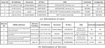
We used the WS-DREAM dataset, which is the QoS dataset of real-world Web services collected by Zheng et al. [37]. The dataset contains 1,873,838 real and valid service invocation records from 339 users on 5825 services, and the available QoS include attributes of response time and throughput. In this study, we used both of the two QoS attributes(response time and throughput) to separately validate our approach. The dataset also includes other information about users and services. The user information and service information are shown in Figure 5. The user information includes [ID, IP Address, Country, IP NO., AS, Latitude, Longitude] and the service information includes [ID, WSDL Address, Service Provider, IP Address, Country, IP NO., AS, Latitude, Longitude]. We use [Country, AS] as the location characteristics of the user and service.
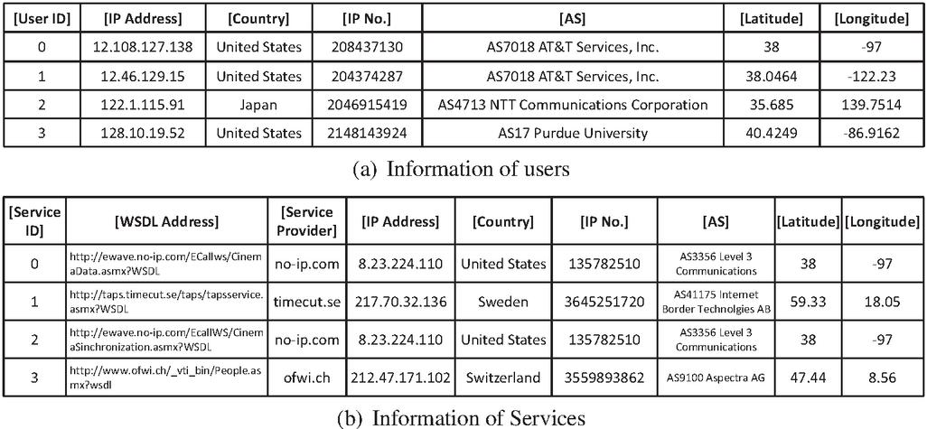
Figure 5 Information of users and services.
4.2.2 Preprocessing
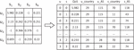
Since the QoS matrix in the real world is extremely sparse, the size of the training set we set is much smaller than that of the testing set. In this paper, we set the matrix densities at 5% to 30% with the step of 5% to verify the effect of the model under different data sparsity. We randomly selected the invocations satisfying the number of target density records as the training set, and the remaining invocations as the test set. For example, there should be 1,974,675 values in the QoS matrix for 339 users and 5825 services. If the current density is 5%, 98,734 QoS values should be known. Then, 98,734 records are randomly selected from the valid records as the training set, and the remaining records as the test set.
In the data preprocessing, we merge the required information from the original data(including the original QoS matrix, user information and service information) and converted them into the form of the invocation record. As shown in Figure 6, the final invocation record converted from QoS matrix is represented as [user ID, service ID, QoS value, user Location, service Location], and locations include country and AS. All IDs and locations in the dataset are assigned unique numbers. We directly use the ID number as the ID encoding, and use the encoding method of Zhang et al. [36] to encode the location information: the categorical encoding of Sklearn is used to convert the country information into integers, and the number of the autonomous system is used as the encoding of AS information.
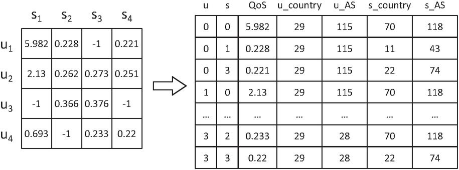
Figure 6 Transformed the matrix to invoked records.
In addition, we need to calculate and store the probability distribution of each user and service. We take the historical QoS distribution of target user and service as the QoS probability distribution in the prediction. In the experiment, the training set is used as historical invocations. According to the QoS interval , the probability distribution is calculated by the historical invocations as the probability distribution characteristics of the corresponding user and service. The selection of will be determined by experiment in Section 5.1.4. The calculation of QoS distribution has been explained in equations 1 and 2 in Section 2.2.
4.3 Comparison Methods
We select the following QoS prediction methods to compare their performance with our method:
• UIPCC(User-Based and Item-Based CF) [37]: This approach is a classic collaborative filtering, which computes similar users and similar services by PCC, and combines them to recommend services to target users. It is the combination of UPCC(User-Based CF) and IPCC(Item-Based FC).
• PMF(Probabilistic Matrix Factorization) [21]: This is a very popular method of recommending fields. MF is to factor the QoS matrix into an implicit user matrix and an implicit service matrix, and PMF is to introduce the probability factor into MF.
• LACF [23]: This is a location-aware collaborative filtering method. The difference of the method and traditional collaborative filtering is that it uses the users close to the target user on the geographic location as similar users, and the services close to the target service on the geographic location as similar services.
• NCF [11]: This method combines CF and MLP, inputs implicit vectors of users and services into MLP, and uses MLP to learn the interaction between potential features of users and services.
• LDCF [36]: This is a location-aware approach that combines collaborative filtering with deep learning. It is a state-of-the-art QoS prediction method, and we take it as our baseline model.
Among these approaches, UIPCC and PMF are content-based and model-based collaborative filtering methods, respectively, LACF and LDCF are location-aware methods, and NCF and LDCF are neural network-related models.
4.4 Evaluation Metrics
The prediction of QoS can be classified as a regression problem, so we use the Mean Absolute Error(MAE) and Root Mean Squared Error(RMSE) to measure the performance of the prediction. MAE and RMSE are defined as:
| (13) | |
| (14) | |
| (15) |
where is the actual QoS value of service observed by user , is the predictive QoS value of service observed by user , and denotes the total number of QoS.
5 Experimental Results
In this section, a series of experiments are designed to answer the four questions raised in Section 4, and the experimental results will be presented and analyzed. Suppose there is no additional explanation in subsections, the parameters of the model we proposed as follows: the number of residual blocks is two, the corresponding number of neurons in the full connection layer is 128 and 64, the number of neurons in the input layer is 256, and the number of neurons in the output layer is 1; The loss function is MAE; The learning rate is set to 0.001; is 20.
5.1 RQ1: Impact of Parameter Settings
5.1.1 Impact of depths
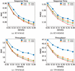
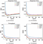
Generally speaking, the increase of the depth of the neural network is conducive to data fitting, while the increase of the number of hidden layers may also lead to gradient descent or gradient disappearance. In our model, the depth of the model is represented by the number of fully connected layers in the main path. Since the hidden layer is composed of residual blocks, and each residual block has two fully connected layers, in this set of experiments, we use the number of residuals to represent different depths. When the number of residual block is , we set the number of neurons in each block as . Response time and throughput were taken as QoS attributes respectively to test the performance of the model at different densities. The specific results are recorded in Table 1, and Figure 7 shows the performance of several models more visually.
Table 1 Experimental results of the models with different Residual blocks number
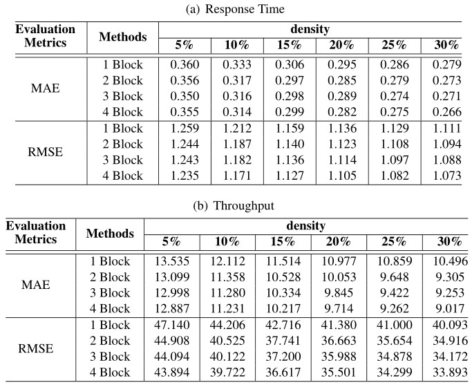
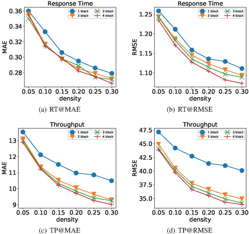
Figure 7 Performance comparison of the models with different numbers of residual blocks.
As can be seen from Figure 7, MAE and RMSE of these models at different depths decreased significantly with the density increased. The reason is the increase of density means the increase of training data. The more data used for learning, the more conducive to the improvement of model performance. Figure 7(a) and Figure 7(b) are the experimental results obtained from experiments with response time as QoS attribute. Under the six densities, the performance is the worst when the number of residual blocks is 1 (the number of hidden layers is 2). While MAE performance of the remaining models was similar, the RMSE performance gap was significant. As the number of network layers increases, the RMSE performance of the model also improves. Figure 7(a) and Figure 7(b) are the experimental results obtained from experiments with throughput as QoS attribute. The MAE and RMSE of the model are lower with more hidden layers, and the network layer number is positively correlated with the model performance. However, in the baseline approach LDCF, there is almost no performance improvement for more than 4 hidden layers [36], which fully demonstrates that the application of our ResNet greatly reduces the problem of gradient disappearance. This allows PLRes to use deeper networks for better results than existing deep learning methods.
5.1.2 Impact of loss function
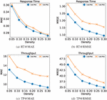
In this set of experiments, we explored the impact of loss functions on the experimental results. According to our performance evaluation method, we used MAE and MSE as loss functions respectively, and use “-” and “-” to represent the corresponding models. In Figure 8, we give results with densities of 5%–30%.
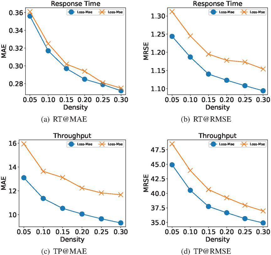
Figure 8 Performance comparison of the models with different loss functions(MAE and MSE).
In Figure 8(a) and 8(b), response time is the QoS attribute; in Figure 8(c) and 8(d), throughput is the QoS attribute. The trend in the four graphs are consistent: the model improved with the density increased, and the test results of - are much better than those of -. We choose MAE as the loss function in our model. On the one hand, - performs better in both MAE and RMSE on the sparse data; on the other hand, RMSE is greatly affected by outliers, and we pay more attention to the general situation.
5.1.3 Impact of learning rate
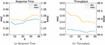
In the process of model learning, the learning rate affects the speed of model convergence to an optimum. Generally speaking, the higher the learning rate is, the faster the convergence rate will be. While the high learning rate often leads to the failure to reach the optimal solution beyond the extreme value, and a low learning rate often leads to local optimum results. We set up the maximum number of iterations for 50. Figure 9 shows the change of MAE and RMSE when the learning rate were 0.0001, 0.0005, 0.001, 0.005 and 0.01 at the density of 5%. The “lr” in the legend stands for “learning rate”.
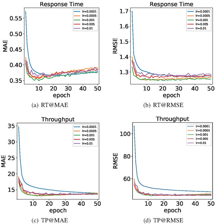
Figure 9 Performance comparison of the models with different learning rates.
In Figure 9(a) and Figure 9(b), response time is the QoS attribute; in Figure 9(c) and 9(d), throughput is the QoS attribute. In the experiment, the models were tested with the testing set when each epoch finished. Therefore, the lowest point of each curve is the optimal result of the corresponding learning rate model, and Table 2 gives the best results of the models under the different learning rates. When the curve in the Figure 9 starts to rise, it indicates that the model starts to overfit. In the four subgraphs, only the curve with a learning rate of 0.0001 is relatively smooth, but its best result is not as good as other models, which is considered the model falls into the local optimal during training. According to the Figure 9(a) and 9(c), it can be observed that when the epoch reaches 10, the other curves with a learning rate greater than 0.0001 have reached the lowest point and then started to rise gradually. In the Figure 9(b) and 9(d), when the epoch reaches 10, the curves gradually tend to be stable. Among these curves, the curve with a learning rate of 0.001 worked best and the curve with the learning rate of 0.0005 is the next. Therefore, when the learning rate is 0.005 and 0.01, we consider the models are difficult to converge due to the high learning rate.
Table 2 Experimental results of different learning rate at density of 5%
| lr | Response Time | Throughput | ||
| MAE | RMSE | MAE | RMSE | |
| 0.0001 | 0.372 | 1.270 | 13.949 | 48.402 |
| 0.0005 | 0.366 | 1.247 | 13.202 | 45.068 |
| 0.001 | 0.356 | 1.244 | 13.099 | 44.908 |
| 0.005 | 0.354 | 1.260 | 13.431 | 45.013 |
| 0.01 | 0.382 | 1.275 | 13.579 | 45.109 |
5.1.4 Impact of
Before the calculation of probability distribution, the number of intervals must be determined first. According to the value of , the range of each QoS interval can be obtained to conduct statistics on the quantity and calculate the probability. This set of experiments is devoted to exploring the influence of on the model effect. At the density of 5%, is set to 5-40 with the step of 5 to conduct model training and testing. The test results are shown in Figure 10.
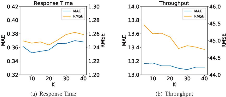
Figure 10 Performance comparison of the models with different values.
Figure 10(a) is the test result of the response time dataset, and Figure 10(b) is the test result of the throughput dataset. With the increase of , the overall trend of model performance in Figure 10(a) is first increased and then decreased, while in Figure 10(b) is generally decreased. The reason may be related to the numerical range of the dataset. The data range for response time is 0-20, for throughput is 0-1000. For most users and services, the range of QoS values is concentrated, which leads to a few intervals with high probability and most intervals with very low probability. With the increase of , the range of QoS value decreases. The QoS values in the set with high probability are scattered, which is conducive to improving the QoS prediction accuracy. However, the low probability interval will be dispersed into multiple intervals with a probability close to 0, which is not conducive to the improvement of the accuracy of QoS prediction. Due to the small value range of response time, the error reduced little, and the disadvantage of increasing is more pronounced. As for the throughput dataset, its data range is larger and error reduction is more obvious, highlighting the advantage of increasing . Therefore, according to the experimental results, we choose the compromise scheme as the model parameter.
5.2 RQ2: Model Effectiveness
In the experiments, we use the same dataset to train the models of comparison methods and PLRes, and test them with the same testing set. For the CF methods need to find similar users or services(UIPCC and LACF), the number of neighbours is set to 10. And for the deep learning method(NCF and LDCF), we set the number of MLP layers as six and the number of neurons in each layer as [256,128,128,64,64,1]. For the MF method(PMF and NCF), we set the number of implicit features as 10. For the parameters that all models need to be used, we set the learning rate to be 0.001, the batch size to be 256 and the maximum number of iterations to be 50. As for the loss function and optimizer, we use the default parameters for each model to ensure that they work well.
Table 3 Experimental results of 6 different QoS prediction approaches
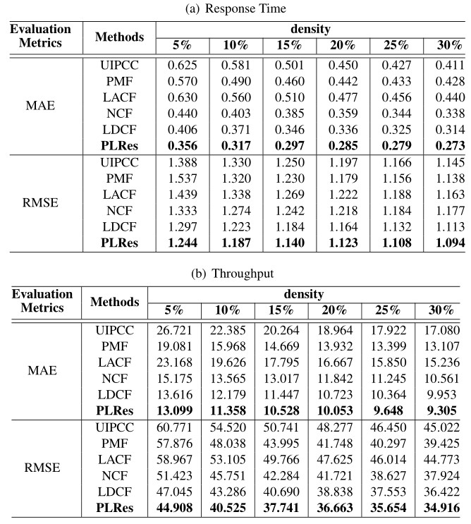
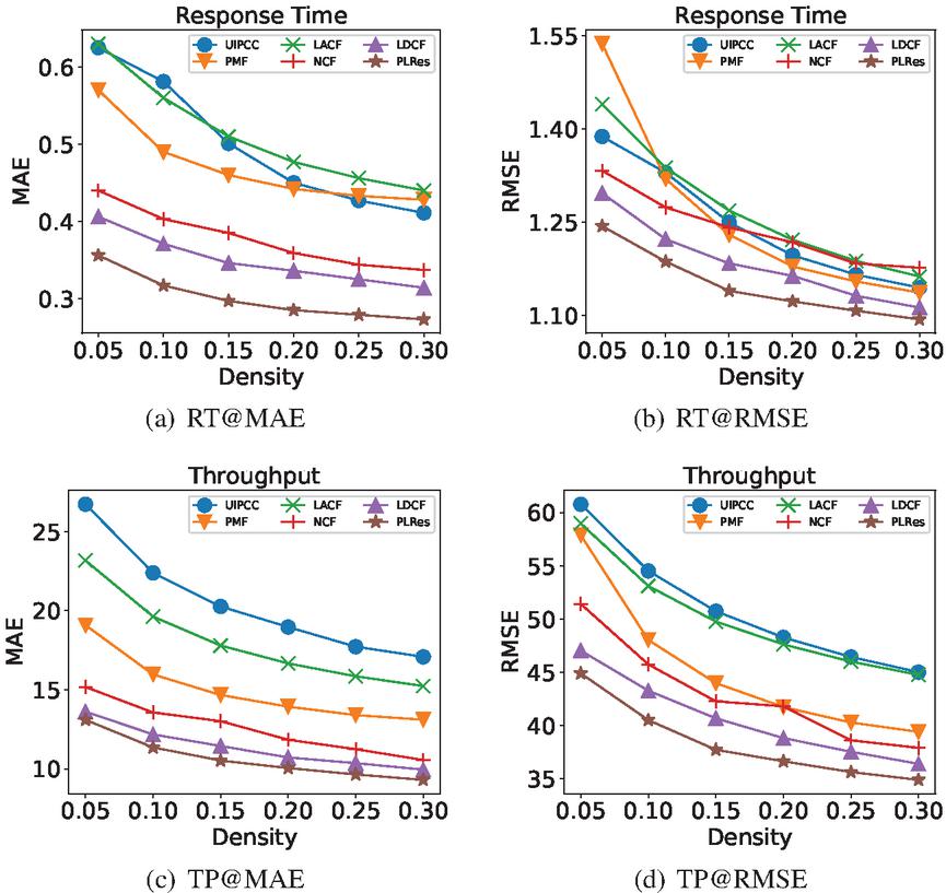
Figure 11 Performance comparison of 6 different QoS prediction approaches.
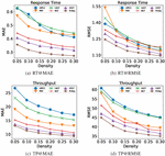
Table 3 shows the detailed test results of the above approaches and our model in six different densities. The QoS attribute used in Table 4(b) is response time, and the QoS attribute used in Table 4(b) is throughput. Figure 11 shows the advantages of our method more intuitively. Figure 11(a) and 11(b) correspond to response time, while Figure 11(c) and 11(d) correspond to throughput. According to the comparison result, with the increase of density and the training data, the MAE and RMSE performance of these methods are all improved, and PLRes always performs best at the same density.
In the experiment using the response time dataset, can be observed in the Figure 11(a), the performance comparison of MAE, the models using deep learning(NCF, LDCF and PLRes) are all below 0.45 at the density of 5%, which perform better than the other three models(UIPCC, PMF, LACF), whose MAE were all above 0.55. Similarly, at other densities, the models using deep learning are more effective. This strongly proves the ability of deep learning to fit nonlinear features in QoS prediction. In terms of the performance comparison of RMSE, it can be observed from the Figure 11(b) that the performance of deep learning models are better than those of CF models at the density of 5% and 10%. It reflects that the CF method is difficult to perform well under sparse density, while the deep learning method greatly alleviates this problem. When the density is greater than 10%, although the CF models gradually outperform the deep learning method NCF, LDCF and PLRes still perform best. This may be related to the introduction of location characteristics and probability distribution characteristics.
In experiments using the throughput dataset, it can be seen from Figure 11(c) and 11(d), the performance of the six methods obviously different. Under the six densities, MAE and RMSE performance relationships is: PLRes LDCF NCF PMF LACF UIPCC. The three methods with better performance are all deep learning methods, which proves the effectiveness of the method using deep learning in QoS prediction.
It is worth mentioning that compared with the baseline model LDCF, PLRes improves MAE performance of response time by 12.35%, 14.66%, 14.17%, 15.37%, 14.24% and 13.22%, RMSE performance by 4.10%, 2.95%, 3.24%, 3.48%, 2.13% and 1.78% respectively under the density of 5%–30%. PLRes improves MAE of throughput by 3.80%, 6.74%, 8.03%, 6.25%, 6.91%, 6.51%, RMSE performance by 4.54%, 6.38%, 7.25%, 5.60%, 5.06%, 4.13% respectively under the density of 5%–30%. Futhermore, we recorded the QoS prediction results of LDCF and PLRes in all tests(QoS attributes of response time and throughput with 6 different densities), and apply the Wilcoxon signed-rank [27] test on the prediction results of PLRes and LDCF to analyze the statistical difference between the two models. The results showed that all the p-value are less than 0.01, which indicates that the improvement of PLRes against LDCF is statistically significant.
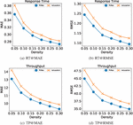
5.3 RQ3: Effect of Probability Distribution
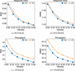
In order to examine the impact of probability distribution, we removed the characteristics of probability distribution, and only took user ID, service ID, user location, service location as the factors to conducted the experiment with the same ResNet model. For the two models, we set the same training data for training, set the maximum number of iterations to 50, and saved the model with the best testing results.
The results of the two models at different densities are shown in Figure 12, the “noPD” in the legend represents the model without probability distribution. Figures 12(a) and Figures 12(b) are the test results for the response time dataset, and Figures 12(c) and Figures 12(d) are the test results for the throughput dataset. Experimental results on the response time dataset show that the model PLRes using the probability distribution features achieves better results, but the difference is close. However, the experiment on the throughput dataset shows that PLRes performs significantly better than noPD.

Figure 12 Performance comparison of PLRes and the model without the probability distribution feature.
From the results, the performance of the model with the probability distribution as the feature has better performance than the model without the probability distribution feature at all six densities. The results fully prove that the introduction of probability distribution is beneficial to improve the performance of the model. The reason is that the probability distribution reflects the user preference and the network stability of users and services. Therefore, the introduction of probability distribution is helpful to reduce the sensitivity to abnormal data and to reduce the overfitting of the model.
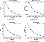
5.4 RQ4: Effect of Location
We will verify the importance of location information to our model in this section. We try to train the model using only ID and probability distribution as characteristics, and compare the testing results with PLRes. We use the “noLocation” stand for a model without the location feature in the resulting figure. Figure 13 shows our test results, in which the test results of PLRes are represented by blue lines, and the test results of the model that only used ID and probability distribution as the characteristics are represented by orange lines. Figure 13(a) is the MAE result and Figure 13(b) is the RMSE result with the QoS attribute response time, Figure 13(c) and Figure 13(d) is the test result with the QoS attribute throughput.
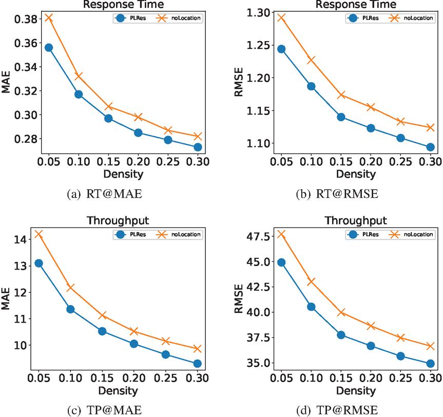
Figure 13 Performance comparison of PLRes and the model without the location feature.
In the four subgraphs, although the performance trends of the two models were similar with the increase of density, the PLRes model using location information always performed better, indicating that location characteristics do have an improved effect on QoS prediction. The reason is that the users in the same region tend to be in similar network status, while users in different regions usually have different network conditions. Therefore, location information can be used as an important reference factor for user similarity, which is also the reason why partial collaborative filtering methods use location information. In addition, location information can reflect the distance between the user and the server, which also tends to affect service efficiency. Even if the invoked service is the same one, users who closer to the server always get better network response and bandwidth.
5.5 RQ5: Effect of Shortcuts
The method of feature reuse in ResNet is to use shortcuts, which add original features directly to trained data. In this section, we discuss the impact of shortcuts on our experimental results. In this set of experiments, we used the DNN and the ResNet to learn the same dataset respectively, so as to prove the effectiveness of the shortcuts. We set the PLRes to use two residual blocks, each of which contains two full connection layers, so in the DNN we set the number of hidden layers to 4. In PLRes, the number of neurons in the two residual blocks is [128, 64], and the number of neurons in each hidden layer in the DNN is [128, 128, 64, 64]. The testing results are shown in Figure 14. Figure 14(a) and Figure 14(b) are the result of the QoS attribute response time, Figure 14(c) and Figure 14(d) are the result of the QoS attribute throughput.
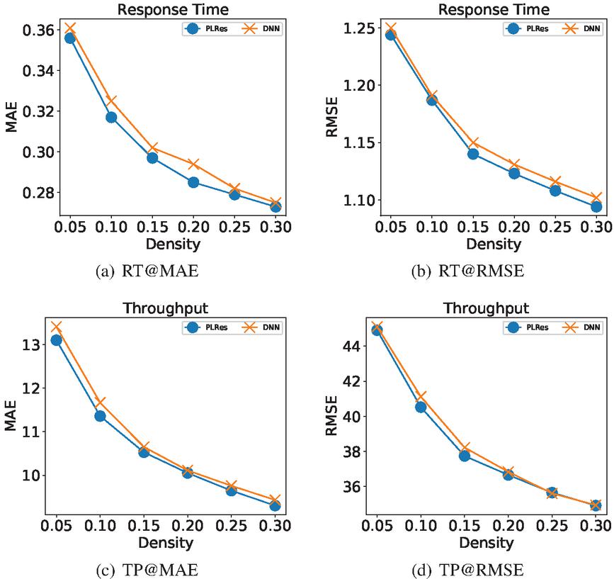
Figure 14 Performance comparison of PLRes and the model without the shortcuts.
In the four subgraphs, the performance of PLRes, which using shortcuts, is better than that of DNN without shortcuts at all densities, which proves that the use of residual network is conducive to the improvement of model performance. Although shortcuts are used to improve the performance of our network in deeper networks, increasing the number of network layers also means increasing the cost of time and space. Therefore, we hope that the introduction of shortcuts can also help improve the performance of the model even when the network is shallow. In this experiment, only 2 residual blocks (4 hidden layers) are used, which also significantly improves the performance, indicating that feature reuse is effective in this model, and the introduction of shortcuts improves the performance of the model. It may be related to the increased number of parameters in shortcuts, but more importantly, the shortcut emphasizes the original feature and strengthens the relationship between features and QoS values.
6 Related Work
In the existing QoS prediction methods, collaborative filtering is the most widely used technology. Collaborative filtering fully considers the user’s preference, so it is commonly used in the recommendation system and performs well in the personalized recommendation.
Collaborative filtering methods can be divided into two categories: memory-based and model-based. The memory-based collaborative filtering method usually achieves the prediction of the target by obtaining similar users or services with similar neighbors. Therefore, memory-based collaborative filtering can be subdivided into user-based, service-based and hybrid-based. Linden et al. [18] help the recommend system find similar items of what the user needs and add them to the recommended sequence by the item-to-item collaborative filtering. Adeniyi et al. [1] used K-Nearest-Neighbor (KNN) classification method to find similar items for recommendation systems. Zou et al. [39] improved the method to integrate similar users and services, proposed a reinforced collaborative filtering approach. In the model-based collaborative filtering, machine learning method is used to study the training data to achieve the prediction of QoS. Matrix factorization is the most typical and commonly used model-based method, which turns the original sparse matrix into the product of two or more low-dimensional matrices. In QoS prediction, matrix factorization often captures the implicit expression of users and services. Zhu et al. [38] propose an adaptive matrix factorization approach to perform online QoS prediction. Wu et al. [28] using the FM(Factorization Machine approach), which is based on MF to predict missing QoS values. Tang et al. [24] considered the similarity as a character, proposed a collaborative filtering approach to predict the QoS based on factorization machines. However, CF can only learn linear features, so many methods begin to consider in-depth learning that can effectively learn nonlinear features.
Deep learning is a subset of machine learning, and it combines the characteristics of the underlying data to form a more abstract and deep representation. Due to its strong learning ability on hidden features, it has been widely used in various recommendation systems [35, 12, 13, 26].
In QoS prediction, some methods combine deep learning with collaborative filtering. Zhang et al. [36] proposed a new deep CF model for service recommendation to captures the high-dimensional and nonlinear characteristics. Soumi et al. [4] proposed a method which is a combination of the collaborative filtering and neural network-based regression model. Xiong et al. [30] proposed a deep hybrid collaborative filtering approach for service recommendation (DHSR), which can capture the complex invocation relations between mashups and services in Web service recommendation by using a multilayer perceptron. Deep learning is also often used in methods using the timeslices of service invocation. Xiong et al. [29] propose a novel personalized LSTM based matrix factorization approach that could capture the dynamic latent representations of multiple users and services. Hamza et al. [15] uses deep recurrent Long Short Term Memories (LSTMs) to forecast future QoS.
In some existing researches [5, 17, 34, 20, 6], location information is considered as one of the characteristics of QoS prediction. Li et al. [16] propose a QoS prediction approach combining the user’s reputation and geographical information into the matrix factorization model. Tang et al. [25] exploits the users’ and services’ locations and CF to make QoS predictions. Chen et al. [6] propose a matrix factorization model that using both geographical distance and rating similarity to cluster neighbors. These approaches have improved the accuracy of QoS prediction, and their experimental results fully demonstrate the validity of location information.
7 Conclusion and Future Work
In this paper, we propose a probability distribution and location-aware QoS approach based on ResNet named PLRes. The model uses ID, location information and probability distribution as the input characteristics. PLRes encodes the ID and geographic location of the users and services, and embedded them into the high-dimensional space. Then all the features(the embedded ID and location features, and the probability distribution) are concatenated into a one-dimensional vector and input into ResNet for learning. We trained the model and conducted experiments on the WS-DREAM dataset. The experimental results fully prove that the features of location and probability distribution are conducive to improving the accuracy of the QoS prediction model. As a deep learning method, PLRes gives full play to its advantages in learning high-dimensional nonlinear characteristics, and compared with the advanced deep learning method LDCF, PLRes effectively alleviates the gradient disappearance problem.
Although the proposed approach improves the QoS prediction performance compared with the existing methods in the experiment, it still has some limitations. On the one hand, the model learns to encode with the existing users and services, so the QoS value prediction of new users and services may not be as accurate as that of the existing users and services. On the other hand, the QoS value is constantly changing. If the training data is out of date, the prediction result will be subject to wide error.
In the future, we will further consider the combination of the current model and collaborative filtering method to make full use of the advantages of collaborative filtering. In addition, we did not consider the time factor for the user to invoke the service in this paper. Since the service is constantly updated, the QoS of different timeslices may change greatly, so the time feature is also necessary in QoS prediction. We will further consider predicting missing QoS value through QoS changes of different time slices in the next work.
Acknowledgements
The work described in this paper was partially supported by the NationalKey Research and Development Project (Grant no. 2018YFB2101201), the National Natural Science Foundation of China (Grant no. 61602504), the Fundamental Research Funds for the Central Universities (Grant no. 2019CDYGYB014), the Natural Science Foundation Projects in Chongqing (Grant no. cstc2019jcyj-msxmX0442).
Notes
1http://wsdream.github.io/
References
[1] D.A. Adeniyi, Z. Wei, and Y. Yongquan. Automated web usage data mining and recommendation system using k-nearest neighbor (knn) classification method. Applied Computing and Informatics, 12(1):90–108, 2016.
[2] E. Ahmad, M. Alaslani, F. R. Dogar, and B. Shihada. Location-aware, context-driven qos for iot applications. IEEE Systems Journal, 14(1):232–243, 2020.
[3] Weihong Cai, Xin Du, and Jianlong Xu. A personalized qos prediction method for web services via blockchain-based matrix factorization. Sensors, 19(12):2749, 2019.
[4] Soumi Chattopadhyay and Ansuman Banerjee. Qos value prediction using a combination of filtering method and neural network regression. In Sami Yangui, Ismael Bouassida Rodriguez, Khalil Drira, and Zahir Tari, editors, Service-Oriented Computing – 17th International Conference, ICSOC 2019, Toulouse, France, October 28–31, 2019, Proceedings, volume 11895 of Lecture Notes in Computer Science, pages 135–150. Springer, 2019.
[5] K. Chen, H. Mao, X. Shi, Y. Xu, and A. Liu. Trust-aware and location-based collaborative filtering for web service qos prediction. In 2017 IEEE 41st Annual Computer Software and Applications Conference (COMPSAC), volume 2, pages 143–148, 2017.
[6] Zhen Chen, Limin Shen, Dianlong You, Chuan Ma, and Feng Li. A location-aware matrix factorisation approach for collaborative web service qos prediction. Int. J. Comput. Sci. Eng., 19(3):354–367, 2019.
[7] T. Cheng, J. Wen, Q. Xiong, J. Zeng, W. Zhou, and X. Cai. Personalized web service recommendation based on qos prediction and hierarchical tensor decomposition. IEEE Access, 7:62221–62230, 2019.
[8] Shuai Ding, Chengyi Xia, Qiong Cai, Kaile Zhou, and Shanlin Yang. Qos-aware resource matching and recommendation for cloud computing systems. Appl. Math. Comput., 247:941–950, 2014.
[9] Feng-Jian Wang, Yen-Hao Chiu, Chia-Ching Wang, Kuo-Chan Huang. A Referral-Based QoS Prediction Approach for Service- Based Systems. Journal of Computers, 13(2):176–186, 2018.
[10] Kaiming He, Xiangyu Zhang, Shaoqing Ren, and Jian Sun. Deep residual learning for image recognition. CoRR, abs/1512.03385, 2015.
[11] Xiangnan He, Lizi Liao, Hanwang Zhang, Liqiang Nie, Xia Hu, and Tat-Seng Chua. Neural collaborative filtering. In Rick Barrett, Rick Cummings, Eugene Agichtein, and Evgeniy Gabrilovich, editors, Proceedings of the 26th International Conference on World Wide Web, WWW 2017, Perth, Australia, April 3–7, 2017, pages 173–182. ACM, 2017.
[12] W. Hong, N. Zheng, Z. Xiong, and Z. Hu. A parallel deep neural network using reviews and item metadata for cross-domain recommendation. IEEE Access, 8:41774–41783, 2020.
[13] I. M. A. Jawarneh, P. Bellavista, A. Corradi, L. Foschini, R. Montanari, J. Berrocal, and J. M. Murillo. A pre-filtering approach for incorporating contextual information into deep learning based recommender systems. IEEE Access, 8:40485–40498, 2020.
[14] Diederik P. Kingma and Jimmy Ba. Adam: A method for stochastic optimization. In Yoshua Bengio and Yann LeCun, editors, 3rd International Conference on Learning Representations, ICLR 2015, San Diego, CA, USA, May 7–9, 2015, Conference Track Proceedings, 2015.
[15] Hamza Labbaci, Brahim Medjahed, and Youcef Aklouf. A deep learning approach for long term qos-compliant service composition. In E. Michael Maximilien, Antonio Vallecillo, Jianmin Wang, and Marc Oriol, editors, Service-Oriented Computing – 15th International Conference, ICSOC 2017, Malaga, Spain, November 13–16, 2017, Proceedings, volume 10601 of Lecture Notes in Computer Science, pages 287–294. Springer, 2017.
[16] Shun Li, Junhao Wen, Fengji Luo, Tian Cheng, and Qingyu Xiong. A location and reputation aware matrix factorization approach for personalized quality of service prediction. In 2017 IEEE International Conference on Web Services (ICWS), pages 652–659. IEEE, 2017.
[17] Shun Li, Junhao Wen, and Xibin Wang. From reputation perspective: A hybrid matrix factorization for qos prediction in location-aware mobile service recommendation system. Mobile Information Systems, 2019:8950508:1–8950508:12, 2019.
[18] Greg Linden, Brent Smith, and Jeremy York. Amazon.com recommendations: Item-to-item collaborative filtering. IEEE Internet Comput., 7(1):76–80, 2003.
[19] An Liu, Xindi Shen, Zhixu Li, Guanfeng Liu, Jiajie Xu, Lei Zhao, Kai Zheng, and Shuo Shang. Differential private collaborative web services qos prediction. World Wide Web, 22(6):2697–2720, 2019.
[20] Wei Lo, Jianwei Yin, ShuiGuang Deng, Ying Li, and Zhaohui Wu. Collaborative web service qos prediction with location-based regularization. In Carole A. Goble, Peter P. Chen, and Jia Zhang, editors, 2012 IEEE 19th International Conference on Web Services, Honolulu, HI, USA, June 24–29, 2012, pages 464–471. IEEE Computer Society, 2012.
[21] Ruslan Salakhutdinov and Andriy Mnih. Probabilistic matrix factorization. In John C. Platt, Daphne Koller, Yoram Singer, and Sam T. Roweis, editors, Advances in Neural Information Processing Systems 20, Proceedings of the Twenty-First Annual Conference on Neural Information Processing Systems, Vancouver, British Columbia, Canada, December 3–6, 2007, pages 1257–1264. Curran Associates, Inc., 2007.
[22] Qibo Sun, Lubao Wang, Shangguang Wang, You Ma, and Ching-Hsien Hsu. Qos prediction for web service in mobile internet environment. New Rev. Hypermedia Multim., 22(3):207–222, 2016.
[23] Mingdong Tang, Yechun Jiang, Jianxun Liu, and Xiaoqing (Frank) Liu. Location-aware collaborative filtering for qos-based service recommendation. In Carole A. Goble, Peter P. Chen, and Jia Zhang, editors, 2012 IEEE 19th International Conference on Web Services, Honolulu, HI, USA, June 24–29, 2012, pages 202–209. IEEE Computer Society, 2012.
[24] Mingdong Tang, Wei Liang, Yatao Yang, and Jianguo Xie. A factorization machine-based qos prediction approach for mobile service selection. IEEE Access, 7:32961–32970, 2019.
[25] Mingdong Tang, Tingting Zhang, Jianxun Liu, and Jinjun Chen. Cloud service qos prediction via exploiting collaborative filtering and location-based data smoothing. Concurrency and Computation: Practice and Experience, 27(18):5826–5839, 2015.
[26] Xuna Wang, Qingmei Tan, and Lifan Zhang. A deep neural network of multi-form alliances for personalized recommendations. Information Sciences, 531:68–86, 2020.
[27] Frank Wilcoxon. Individual comparisons by ranking methods. In Breakthroughs in statistics, pages 196–202. Springer, 1992.
[28] Yaoming Wu, Fenfang Xie, Liang Chen, Chuan Chen, and Zibin Zheng. An embedding based factorization machine approach for web service qos prediction. In E. Michael Maximilien, Antonio Vallecillo, Jianmin Wang, and Marc Oriol, editors, Service-Oriented Computing – 15th International Conference, ICSOC 2017, Malaga, Spain, November 13–16, 2017, Proceedings, volume 10601 of Lecture Notes in Computer Science, pages 272–286. Springer, 2017.
[29] Ruibin Xiong, Jian Wang, Zhongqiao Li, Bing Li, and Patrick C. K. Hung. Personalized LSTM based matrix factorization for online qos prediction. In 2018 IEEE International Conference on Web Services, ICWS 2018, San Francisco, CA, USA, July 2–7, 2018, pages 34–41. IEEE, 2018.
[30] Ruibin Xiong, Jian Wang, Neng Zhang, and Yutao Ma. Deep hybrid collaborative filtering for web service recommendation. Expert systems with Applications, 110:191–205, 2018.
[31] Yueshen Xu, Jianwei Yin, ShuiGuang Deng, Neal N. Xiong, and Jianbin Huang. Context-aware qos prediction for web service recommendation and selection. Expert Syst. Appl., 53:75–86, 2016.
[32] Hong-Jian Xue, Xinyu Dai, Jianbing Zhang, Shujian Huang, and Jiajun Chen. Deep matrix factorization models for recommender systems. In Carles Sierra, editor, Proceedings of the Twenty-Sixth International Joint Conference on Artificial Intelligence, IJCAI 2017, Melbourne, Australia, August 19–25, 2017, pages 3203–3209. ijcai.org, 2017.
[33] Yuyu Yin, Lu Chen, Yueshen Xu, Jian Wan, He Zhang, and Zhida Mai. Qos prediction for service recommendation with deep feature learning in edge computing environment. MONET, 25(2):391–401, 2020.
[34] Y. Yuan, W. Zhang, and X. Zhang. Location-based two-phase clustering for web service qos prediction. In 2016 13th Web Information Systems and Applications Conference (WISA), pages 7–11, 2016.
[35] Shuai Zhang, Lina Yao, Aixin Sun, and Yi Tay. Deep learning based recommender system: A survey and new perspectives. ACM Comput. Surv., 52(1), February 2019.
[36] Yiwen Zhang, Chunhui Yin, Qilin Wu, Qiang He, and Haibin Zhu. Location-aware deep collaborative filtering for service recommendation. IEEE Transactions on Systems, Man, and Cybernetics: Systems, 2019.
[37] Zibin Zheng, Hao Ma, Michael R. Lyu, and Irwin King. Qos-aware web service recommendation by collaborative filtering. IEEE Trans. Serv. Comput., 4(2):140–152, 2011.
[38] Jieming Zhu, Pinjia He, Zibin Zheng, and Michael R. Lyu. Online qos prediction for runtime service adaptation via adaptive matrix factorization. IEEE Trans. Parallel Distrib. Syst., 28(10):2911–2924, 2017.
[39] Guobing Zou, Ming Jiang, Sen Niu, Hao Wu, Shengye Pang, and Yanglan Gan. Qos-aware web service recommendation with reinforced collaborative filtering. In Claus Pahl, Maja Vukovic, Jianwei Yin, and Qi Yu, editors, Service-Oriented Computing – 16th International Conference, ICSOC 2018, Hangzhou, China, November 12–15, 2018, Proceedings, volume 11236 of Lecture Notes in Computer Science, pages 430–445. Springer, 2018.
Biographies

Wenyan Zhang received her bachelor degree from Chongqing University, China in 2019 and went on to pursue her master degree at Chongqing University in the same year. Her research interests are in service discovery and recommendation.

Ling Xu is an Associate Professor at the School of Big Data & Software Engineering, Chongqing Univeristy, China. She received her B.S. degree in Hefei University of Technology in 1998, and her M.S. degree in software engineering in 2004. She received her Ph.D. degree in Computer Application from Chongqing University, P.R. China in 2009. Her research interests include mining software repositories, bug rediction and localization.

Meng Yan is a post-doctoral research fellow in College of Computer Science and Technology, Zhejiang University. He received his PhD degree in June 2017 from the School of Software Engineering, Chongqing University. His currently research focuses on how to improve developer’s productivity, how to improve software quality and how to reduce the effort during software development by analyzing rich software repository data. More information at: https://yanmeng.github.io/

Ziliang Wang received the B.S. degree from Nanchang Hangkong University, Jiangxi, China, in 2017. He is currently pursuing the Ph.D degree in software engineering in Chongqing University, Chongqing, China. His current research interests include service computing, smart city and system structure.

Chunlei Fu is currently a senior engineer at School of Big Data & Software Engineering, Chongqing University. He received his PhD degree at in School of Automation, Chongqing University, China, in 2014. He received a postdoctoral training at the school of computer science in Chongqing University, studying Knowledge-Based Software Engineering. His major research interests include Knowledge Graph, Service Computing, and Software Engineering.
Journal of Web Engineering, Vol. 20_4, 1189–1228.
doi: 10.13052/jwe1540-9589.20415
© 2021 River Publishers