Machine Learning Modeling: A New Way to do Quantitative Research in Social Sciences in the Era of AI
Jiaxing Zhang1, 3 and Shuaishuai Feng2,*
1The Institute of Social Development Studies, Wuhan University, China
2School of Sociology, Wuhan University, Wuhan, Hubei, China
3Shenzhen Qianhai Siwei Innovation Technology Ltd. Co., Shenzhen, China
E-mail: whu-fs@whu.edu.cn
*Corresponding Author
Received 17 November 2020; Accepted 23 November 2020; Publication 05 March 2021
Abstract
Improvements in big data and machine learning algorithms have helped AI technologies reach a new breakthrough and have provided a new opportunity for quantitative research in the social sciences. Traditional quantitative models rely heavily on theoretical hypotheses and statistics but fail to acknowledge the problem of overfitting, causing the research results to be less generalizable, and further leading to Social predictions in the social sciences being ignored when they should have been meaningful. Machine learning models that use cross validation and regularization can effectively solve the problem of overfitting, providing support for the Social predictions based on these models. This paper first discusses the sources and internal mechanisms of overfitting, and then introduces machine learning modeling by discussing its high-level ideas, goals, and concrete methods. Finally, we discuss the shortcomings and limiting factors of machine learning models. We believe that using machine learning in social sciences research is an opportunity and not a threat. Researchers should adopt an objective attitude and make sure that they know how to combine traditional methods with new methods in their research based on their needs.
Keywords: Era of artificial intelligence, machine learning modeling, overfitting, prediction studies.
1 The Development of Artificial Intelligence and Machine Learning Algorithms
The rate at which technology advances has exceeded the imagination of most. It took only a few decades to go from the information age to the internet age, immediately followed by the era of big data. People are still getting accustomed to big data, and, suddenly, people are saying that it is now the era of artificial intelligence. Starting from 2016, Yang Lan and her team spent over a year visiting over 30 top artificial intelligence laboratories and research facilities around the world and interviewing over 80 top researchers in the field. In 2017, she wrote and published In Search of Artificial Intelligence. The same year, in July, in order to strategically push the development of artificial intelligence and to become a country leading in new and powerful technologies, the state department released the “Development Plan on the New Generation of Artificial Intelligence”. This is the first document published by the Chinese government on artificial intelligence, indicating that AI has officially become an important strategic direction for future development. Some scholars explained the phenomenon as such: the fourth industrial revolution is a revolution of intelligence. The cutting edge of intelligence technology is artificial intelligence, which is quickly becoming the centerpiece for the structural transformation and upgrade of technology, culture, society and economy. (Ding et al., 2018:1) It can be predicted that artificial intelligence will be used in almost every technology and application in the future, and will be deeply integrated with our society and economy. Every field can utilize artificial intelligence to automate large-scale activities that traditionally need human intelligence, and this will fundamentally alter the life style and the mode of production of human beings. Certainly, this change will be both a significant challenge and opportunity to the many researchers in the field of social sciences who analyzes the complexities of human societies.
From history, we can observe that the paradigm shifts in social science studies have been closely related with the advancement of technology. Limited by research methods and data analysis methods, the development of social sciences before the Internet era was slow. For instance, social scientists have known that human society is a Complex Adaptive System, but the pervasive method of studying back then was to manually split the system into smaller parts such as politics, economics, cultures, etc. Reductionism is used in research, but the results are obviously flawed. The internet age gave social scientists new ways to do research. Researchers started using network analysis to study human behavior and the society, achieving better results. Then comes the era of big data and the emergence of computational social sciences. Social scientists saw a beacon of hope to break the social science bottleneck. As social scientists debated on whether computational social science could incite a real social science revolution, artificial intelligence reached a new breakthrough and could effectively be combined with big data. Artificial intelligence exceeded peoples’ psychological threshold and stepped into the technological spotlight, marking the start of the era of AI.
The resurgence of artificial intelligence can in part be attributed to deep learning (DL) algorithms. Deep learning is a new research direction under the broader field of machine learning (ML). Machine learning is vital to achieving more intelligent artificial systems. To date, machine learning has a complete set of theories and methods. In terms of research methods of social science, machine learning can be used to train models, then select, categorize, or cluster items, making machine learning a great tool with many advantages for quantitative research. On this basis, this paper focuses on discussing and answering the following three questions: First, since new technologies and methods are often used to solve problems that more traditional methods cannot be solved, then what can machine learning do that traditional methods cannot? Second, as a way to conduct quantitative research in the social sciences, what new characteristics does machine learning modeling have compared to traditional modeling? Third, everything has its pros and cons. What are the disadvantages to using machine learning modeling?
2 Overfitting and the Difficulties of Prediction
Science, whether it is natural sciences or social sciences, focuses largely on analyzing the change in quantity and relation to find the cause and effect behind a particular phenomenon. The main mission is to conclude some cause-and-effect rule of nature or of society. Although it is clear that societal systems are characteristically complex, due to many factors such as subject heterogeneity, interaction between several factors, and the nonlinearity of interactions and relations, researchers never gave up on exploring causal predictions. As early as the last century, in the 40 s, Kaplan proposed to increase predictions in the social sciences. He argued that compared to natural phenomena on a smaller scale, social behavior is easier to predict. “The reason humans differ from atoms and molecules is because to a certain degree, human behavior can be predicted by the rules that humans themselves have created.” (Kaplan, 1940:493). Yet, over the last hundred years social scientists have not progressed in any tangible way regarding cause and effect predictions. In particular, quantitative researchers who aim to prove scientism put more effort into describing the data and falsifications, and are in general less proficient in (or unable to perform) cause and effect predictions. (Chen et al., 2020). The definition of social prediction is as follows: Using local data in space and time that present social phenomena or processes, based on appropriate model methods, accurate quantitative measurement of unknown information outside of time and space, so as to provide information and basis for social decision-making and research. The reason quantification in the social sciences is often criticized is because the research results can hardly be generalized. Given some different data, difference variables, or even different sequencing of the data, the study could produce completely opposite results. Even after more than decades of development, with many complex quantitative models, quantitative research still has the same drawbacks. In reality, this inability to generalize stems from traditional quantitative research models not solving the overfitting problem. (Babyak, 2004; McNeish, 2015). Take a classic example in the social sciences using a linear regression model (Xie, 2010), the basic formula is as follows:
| (1) |
In the formula, is the intercept term (also called the constant term), is the regression coefficient of the ith predicted variable, is the observed value when the ith term is applied to the target variable, is the observed value when the ith term is applied to the ath predicted variable, and is the residual term. Ordinary least square (OLS) is the most commonly used prediction method in linear regression, and normally it attempts to predict the coefficients of the regression model by minimizing the error between the observed value and the predicted value of the target variable, thus providing the most accurate linear prediction given the current data (Fomby et al., 1984; Chartterjee and Hadi, 2006). However, more and more researchers discovered that due to an internal problem, OLS has some error when used to predict the regression coefficients (Chen et al., 2010; Anning, 2012) and is very likely to overfit (Hawkins, 2004; Yarkoni and Westfall, 2017). The regression model does not fit well when used on different data in the same set, or future observed data. The reason is because too many variables are added into the model based on theory and statistical knowledge, weakening the simplicity of the model and causing the model to be too “sensitive”. This in turn limits the ability for the model to generalize and predict to a great extent.
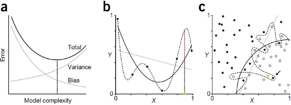
Figure 1 Overfitting in regression and classification (source: Lever, Krzywinski and Altman, 2016).
In September 2016, Lever, Krzywinski, and Altman co-published an article titled Model selection and overfitting on Nature, specifically discussing the problem of overfitting in scientific studies. They proposed that one could look at the difference between the model output and the truth value (bias) and the difference between the model output and the expected output (variance) to evaluate how well fit a model is. These two evaluations directly affect the error of the model. (error bias variance). Bias and variance are both affected by the complexity of the model (as shown in Figure 1a). An overly simple model can have high bias and low variance (underfitting), while in contrast, an overly complex model usually has low bias and high variance (overfitting). Overfitting and underfitting are common problems seen in regression and classification. For instance, a straight line and a model with normally distributed noise display a third-order polynomial mismatch (as shown in Figure 1b). In comparison, the fifth-order polynomial is overfitted, and the coefficients of the model are heavily affected by noise. As we expect, the third-order polynomial provides the best results, even though the high noise conceals the actual tendency. If our goal is to bring down the total error, then we can choose to use an even simpler model (for example, a second-order polynomial.) This is similar to classification. For instance, a complex decision boundary can perfectly separate the data in the training set, but because of its high level of noise, it can produce many classification errors (as shown in Figure 1c). In regression and classification problems, overfitted models perform great on training data, but often perform extremely poorly for new data.
Perhaps a target map can more clearly demonstrate the relations between bias, variance, overfitting, and underfitting. As shown in Figure 2, the bullseye is a model that predicts perfectly. The further away from the bullseye, the lower the prediction accuracy of the model. The crosses on the target map represent a data set when run through a particular model. The vertical axis is the model’s bias: a higher bias means the predictions are further away from the target, while a low bias means the predictions are close to the bullseye; the horizontal axis is the model’s variance. A high variance suggests a higher spread in the fitting process. As for the problem of overfitting, in the four situations, the ideal is to have low bias and low variance like the model on the top left. The model on the bottom right is the worst, with high bias and high variance. An underfitted model has high variance and low bias, and an overfitted model has high bias and low variance.
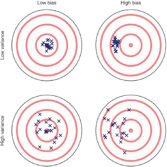
Figure 2 Bias-Variance target map (source: Yarkoni and Westfall, 2017).
In a traditional OLS regression model, the coefficients of the model are calculated by minimizing the cost function, i.e., minimizing the squared distance between the observed values and the predicted values, which increases the fit of the model. (McNeish, 2015). In other words, OLS modeling intrinsically controls bias to lower the prediction error of a model. However, as more and more variables are added to the model, the variance of the model increases, causing the model to fit well on the training set but perform and predict poorly given any other data set. This is, again, the overfitting problem we have been emphasizing. Overfitting causes the model to overestimate the regression coefficients while underestimating the standard error, giving some redundant variables in the model the ability to control predictions. The model can only be used for the training data and cannot be generalized (Li-Jin et al., 2020).
We believe that no matter from the perspective of using a concrete method or the perspective of cause-and-effect analysis, overfitting is a problem that cannot be ignored by quantitative researchers. Unfortunately, the social science community in China has paid little attention to the problem of overfitting. If we search for the term “overfitting” in the CKNI (Chinese National Knowledge Infrastructure) database, there are 377 papers that mention overfitting, among which only one pertains to the social sciences, which was published in the online version of Advances in Psychological Science on August 24th, 2020.
To date, the OLS regression model is still the mainstream model used in quantitative research in the social sciences. In addition, to analyze cause and effect, the control variates method is the most widely used statistical mechanism, isolating the variables that can change both the prediction variable and the target variable. From the 149 quantitative papers published on Sociological Studies from 2010 to 2019, we discovered a few things. First, the control variates method is the single most frequently used statistical mechanism. In the 149 quantitative papers, 132 used at least one control variable, suggesting a use rate of 88.59%. Second, control variables are used in places where they do not need to be. Out of the 132 quantitative papers that use at least one control variable, 13.64% use 1 to 3 variables, 47.73% use 4 to 6 variables, 29.55% use 7 to 9 variables, 6.82% use 10 to 12 variables, and 2.27% use 13 or more variables. In particular, one paper used a shocking 21 control variables. More and more quantitative researchers worry that without exhausting all the variables, they will construct an incorrect model and reach a wrong conclusion (Antonakis et al., 2010). This brings them to use a method that we call “over-control”. As we mentioned above, the more control variables, the higher the variance, which causes overfitting.
In comparison, western scholars noticed the problem of overfitting earlier, and carried out a series of discussions on the relationship between predicting variables and overfitting models. Babyak (2004) suggested a few techniques that could be used to prevent overfitting, for instance, gathering more data, combining variables to reduce the number of variables in a model, and the most interesting and insightful suggestion – shrinkage and penalization. Babyak argued that the other two techniques are not reliable enough and the model could still be overly optimistic. Shrinkage and penalization can tweak the level of optimism and be used to calculate how the model might function in the real world. Shrinkage and penalization uses algorithms and statistical knowledge to add a new combined metric to the model that represents the fitted value of the regression model. Babyak also boldly predicted that in the future, most models will use shrinkage and penalization. More advanced statistical knowledge and algorithms will bring with them more complex shrinkage algorithms, such as maximum likelihood penalty (see Harrell, 2001:207–210). This is a method that pre-shrinks regression coefficients and fitting, so the model can be better copied. The advantage of penalization is that we can adjust parts of the model, therefore adjusting the complexity (such as the interactions between different factors and nonlinear interactions).
In recent years, with the rapid advancement of artificial intelligence, machine learning algorithms are also advancing and evolving. Machine selection and modeling are increasingly used in quantitative studies in the social sciences because of its unique advantages. On one hand, compared to traditional regression methods such as OLS which lowers error by reducing bias and introducing variance, machine learning modeling reduces error by using regularization, which reduces variance by introducing some bias. Then, by fitting the model more properly, the model turns out to be more precise. (Athey and Imbens, 2016). On the other hand, cross validation used in machine learning is now a widely accepted way to solve the problem of overfitting. (Lever et al., 2016).
3 Machine Learning Modeling: Ideas, Goals, and Methods
With communication via computers and the internet being used ubiquitously in everyday life, the traditional problem of collecting data in social sciences is in most cases much less relevant. Digital traces data, social media data, internet text data, positional data, and more traditional large-scale surveys combined make a very solid database for quantitative research in the social sciences (Hao et al., 2017). Researchers can use faster, more convenient, and less expensive ways then before to acquire and store data. However, data itself cannot present useful information. It needs to be studied, researched, or analyzed using some theory or technology before it has value. Machine learning is one great way of combining technology and data to find valuable information in a data set. Machine learning can create a model out of the abstract data and predict the coefficients, thereby finding information valuable to humans from data. (De-Yi, 2018:95). Machine learning, which is based on computer science and statistics, has now become one the most rapidly developing fields in the world and is core to the development of artificial intelligence and data science. Machine learning got to where it is today because of new computer algorithms and statistical theories, and because available data and computational power are both growing. Jordan and Mitchell (2015) defined machine learning as follows: the basic concept of a machine learning algorithm is searching for a best, most optimized algorithm out of a huge number of candidate algorithms with experience and training. From the perspective of social sciences, these are certain algorithms that can take in some data and then do a job such as clustering, sorting, or predicting (Athey, 2018). Furthermore, machine learning helps researchers through the means of calculation to improve the fit of the model using the collected empirical data. Its fundamental task is to analyze and model intelligently based on empirical data, and then find results with certain academic value from the data.
3.1 Supervised Learning Idea: Cross Validation
Strictly speaking, compared with high level statistical models such as instrumental variables (IV) and differences-in-differences (DID), machine learning is not a model with a strict boundary concept. It is more a mode of thinking and a set of methods that reduces the generalization error (the error between predicted and real data) of the model through a certain sequence of procedures. It prevents overfitting to improve the ability for the model to be generalized (predicting real world results). Cross validation is one such idea used commonly in machine learning modeling and designing coefficients. Cross validation, as the name suggests, uses the same data set repeatedly, splitting the data set into training sets and test sets. (To ensure the efficacy of training, usually a 2:8 ratio or a 3:7 ratio is utilized, which means 80% of the data set is used in training and 20% is used in testing, or 70% is used in training and 30% is used in testing.) (If the given sample data is sufficient, it is better to divide the data set into three parts: training set, validation set and test set. The training set is used to train the model, the verification set is used to select the model, and the test set is used to evaluate the construction model.). Based on this idea, the model is repeatedly trained and tested. The steps are: first, use the training set to train the model. Use the error of the model to retrain the model iteratively, thus getting a model that better fits the dataset. Use the test sets to test the model (using criteria such as fitness and prediction accuracy). With multiple training and test sets, a set used for training can next time be used for testing. This is what “cross” stands for in cross validation. The test set needs to satisfy at least two requirements: one, the test set has to be big enough to have statistical significance; two, the test set needs to be able to represent the entire data set. In other words, the test set needs to have the same distribution of characteristics as the entire data set.
Concretely, there are mainly three ways to split up a data set to be used with cross validation. First is simple cross validation (dichotomy). The simplicity refers to it being simple in relation to the other methods. First, we split the data set into two parts (e.g., 70% training set and 30% test set). Then, we use the training set to train the data, and use the test set to evaluate the model and the coefficients. Right after, we reshuffle the data set and reselect the training and test sets to continue to train and evaluate the model. At last, we choose the model which is determined by the loss function to be the best. The second way is K-folder cross validation. Different from simple cross validation, K-folder cross validation splits the data set into K parts, randomly choosing K-1 parts as the training set and the remaining one part as the test set. Afterward, repeat the process by randomly choosing another K-1 parts as the training set. After K rounds, choose the optimal model determined by the loss function. The third way is leave-one-out cross validation. This is an exception of the second method. K here is equal to the sample size N. Every time, N-1 samples are used as the training set, with the one remaining sample used as the test set. This method is usually used when there is very little data (e.g., when N is less than 50). In practical research, what cross validation variance to be used depends on the amount of data there is.
3.2 Machine Learning Modeling Goal: Minimizing Loss
Modeling is a core task in machine learning. Machine learning modeling is, simply explained, a way to transform a machine learning problem into a mathematical problem. Using the common “education level to income” question as an example, we will explain how a machine learning problem is transformed into a mathematical problem. If we collected via questionnaire the data of a group of people’s education level (X) and income (Y), we get a data set . Through literature review we observe that there seems to be some kind of linear relationship between the education level and income of an individual. Suppose the formula for this linear relationship is , in which the coefficients and are yet to be determined. This linear formula we came up with is what is called modeling in a machine learning task. By training this model with data, we can solve for what the coefficients should be. Since there are two unknowns, we can use the same procedure as how one would solve a linear function, using two pairs of data to find the coefficients. However, the problem with this method is that those coefficients can describe the two pairs of data very well, but are not applicable to all the other pairs in the data set. Therefore, we need to find coefficients that can better fit all the pairs in the data set, and a simple linear solution is apparently not the best solution. With that, we can define a loss function that defines the error using a mathematical boundary model (which is also the loss function in OLD regression):
| (2) |
This target function depicts the difference between the predicted values and the real values of coefficients and . The goal of machine learning is to minimize this loss function , and this is where model optimization comes in, also known as training. Once we finish training using the data set, we can predict Y using the given X to a certain degree, which is also known as testing. Given a certain loss function, we hope to obtain a set of coefficients that minimizes the loss function, and this is what is known as mathematical optimization in machine learning. However, due to the limitations in size of the data set, it is impossible to test all the sets of data to find this set of coefficient values to minimize the loss function . That is to say, a global optimum is difficult to obtain; the search of a local optimum is thus the aim of machine learning modeling as a compromise. Let us assume the relation between X and Y is shown in Figure 3. Suppose there is a set of coefficients such that any value of satisfies Formula 3. Then, is the global optimum (Figure 3a). If there exists an such that all the values that satisfy also satisfy Formula (2), then is a local optimum (Figure 3b). A local optimum is not necessarily a global optimum, but is nonetheless a solution within a particular range, meaning it is definitely not a bad solution. When the realistic situation is overly complex with too much information to process, finding a local optimum instead of a global one is used most often in machine learning tasks (Shengyong and Yongbing, 2018:21–23). Although the above example looks simple, most machine learning tasks are based around representing the problem with an appropriate mathematical formula then using math to optimize the loss function, finding the coefficients and predicting new data sets.
| (3) |
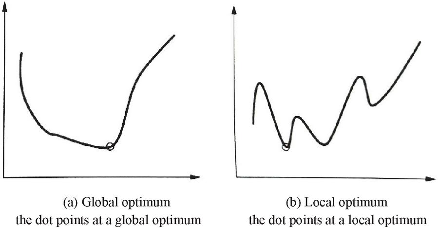
Figure 3 Optimization in Machine learning modeling.
3.3 Machine Learning Modeling: Supervised and Unsupervised
After a few decades of development, machine learning technology has formed a relatively complete set of methods. Based on whether the training set has its characteristics labeled, learning tasks can be categorized into supervised learning, unsupervised learning, and weakly supervised learning. Each category is best suited for certain areas of learning. Supervised learning is good at classification and regression prediction, unsupervised learning is best at clustering, and weakly supervised learning can be applied in any of the three mentioned above. In particular, supervised learning is highly appropriate for predictive social science research. (Hang, 2012:3–6, Yunsong et al., 2020).
Supervised learning is the most important method in machine learning. Most machine learning tasks as of today are supervised. Supervised learning means that the training set is labeled with characteristic data, and the algorithm uses those labeled data as it trains its model. Once the model is trained, the test set is used to evaluate the model. In simpler terms, we already know the input Xi and output Yi even before the model has been trained. Supervised learning simply comes up with a best fit model that accurately projects the input to the output such that when given new data, a prediction can be made. Since the training data is labeled, supervised learning is relatively easier to model and has lower complexity, often reaching higher accuracy. Using the “education level to income” problem again, if 10,000 samples are collected, and each sample has 5 characteristics (gender, name, education level, parents’ education level, income), we first need to manually label the all the characteristics besides income x1 to x4, and label income as y. We randomly select 7,000 samples as the training set, and the remaining 3,000 as the test set. Using certain methods to train the model, such as normalization, supervised learning can automatically eliminate redundant variables (such as x1: gender), and then evaluate the model, eventually obtaining the model with the best prediction accuracy. Common supervised learning algorithms include regularized regression, support vector machines, K-nearest neighbors (KNN), decision trees, and random forest.
Different from supervised learning which is based on manually labelled data, unsupervised learning algorithms learns and self-reinforces, finally generalizing its learning process into a model. Because the training data is unlabeled, it is harder for unsupervised learning models to be highly accurate, which makes unsupervised learning less useful than supervised learning in practice. However, it brings a lot to the table by opening many possibilities in quantitative research. For instance, unsupervised learning can be used to transform or lower the data dimensions of high dimensional and non-structural data such as literature, images, music, and videos which traditional methods cannot. No labeling is needed in this process. This method can be used to expand upon the finding of empirical data which traditional social science research uses. Furthermore, we can try to cluster similar data into groups and put different data into different groups to automatically categorize items, helping researchers find some sort of pattern in seemingly unstructured data. This is what clustering is in unsupervised learning. Academia has been finding value in unsupervised learning in recent years. In 2015, the “Big Three in Deep Learning”, LeCun, Bengio, and Hinton published in Nature that the procedure of how an unsupervised learning task comes up with a model is similar to how humans learn. “Humans and animals learn in largely the same way as unsupervised learning: we observe. We are not taught the names of every object in the world. Thus, if we look further, unsupervised learning will become increasingly important.” Common unsupervised learning algorithms include the clustering algorithm, community detection, and latent semantic analysis.
Labeling data is a practice of high cost. In supervised learning, a lot of tasks lack the strong supervised information such as all truth labels, especially dealing with large data samples. Unsupervised learning often has many limitations in its actual practice due to the lack of manually labeled data. To this end, the concept of weakly supervised learning was proposed. Weakly supervised learning reduces the amount of labeled data needed and uses some aspects of human supervised learning to increase the efficacy of unsupervised learning (Zhou, 2018). Weakly supervised learning is weak when compared to supervised learning. Different from supervised learning, only part of the data is labeled manually in a weakly supervised learning task. The rest is raw, unlabeled data. In other words, weakly supervised learning is a form of indirect learning. The results of machine learning are not given directly to the model, but to some messengers in between. Some representative weakly supervised learning models are semi-supervised learning, transfer learning, and reinforcement learning. In 2016, DeepMind’s AlphaGo used reinforcement learning to beat the world chess champion Lee Sedol, winning four out of a total of five games. Reinforcement learning has since gotten the attention of academia and the industry. To date, reinforcement learning has been used effectively in computer games, self-driving cars, recommendation algorithms, robots, and many other fields. Google, Facebook, Baidu, Microsoft, and other big tech companies are also putting reinforcement learning on their list of key technologies to develop. (Deyi, 2018:107).
3.4 Example of Supervised Learning: Regularized Regression
We mentioned above that regularization can effectively solve the problem of overfitting, and it so happens that regularization is a key algorithm in supervised learning. In theory-driven multiple regression modeling, very often there is not a linear relationship between the one or more predicted variables and the goal variable. This violates the “entities should not be multiplied without necessity” rule in Occam’s Razor, causing the model to be overly sensitive. The idea behind Occam’s Razor is an important driving factor in regularization in machine learning. Regularization, simply put, adds a penalty term in the classic OLS loss function, using an algorithm to get rid of the unnecessary variables, eventually constructing a model with lower average error and lower complexity. The basic working is as follows: The penalty term is usually a monotonically increasing function that describes model complexity, and the loss function tries to minimize error. The loss function and the penalty term form a tug-of-war relationship, the smaller the loss function, the more complex the model, and the bigger the penalty term. To make the penalty term small, the model cannot be too complicated, which in term prevents overfitting from happening. The formula for regularization is as follows:
| (4) |
In the formula, is the loss function after adding in a penalty term, is the loss function of a normal OLS, is the penalty term coefficient (how much to penalize), the bigger the coefficient, the higher the penalty, and the tighter the restraint. It is worth mentioning that when is 0, the penalty term is 0, and is equivalent to the loss function of a normal OLS. is the penalty function, and depending on the different penalty functions, different regularization methods can be used respectively. There are two common penalty functions: L1 norm and L2 norm , respectively used with Lasso regression (least absolute shrinkage and selection operator), and ridge regression. In ridge regression, the sum of squared regression coefficients is the penalty function and can effectively compress the coefficients toward the direction of 0 instead of compressing any particular variable coefficient to 0. This makes it easy to overly compress important coefficients (Hesterberg et al., 2008). This in some part limits the usability of ridge regression. In comparison, Lasso regression solves the above-mentioned problem that ridge regression has, and is therefore more widely used. The idea behind Lasso regression is sparsity. By changing many variable coefficients to 0, a lot of redundant variables are erased, keeping only the prediction variables most relevant to the target variable, simplifying the model while keeping the most important data in the data set. For quantitative social science research, Lasso regression “is a great and stable variable filter, and can be used to build prediction models with better generalizability.” Especially in new research with insufficient theories, “researchers should use methods like these to avoid overfitting to the data at hand and finding a rule that is more applicable on the whole” (Lijin et al., 2020). To date, Lasso regression is used in many fields such as clinical medicine (Kohannim et al., Demjaha et al., 2017), financial investment (Cuixia et al., 2016), and local finance (Yan et al., 2020) to do prediction research with pretty good results. From a technical and application perspective, as machine learning matures, many software systems are able to use Lasso regression in modeling, such as the R language, Python, and Stata 15.0.
4 Conclusions and Discussions
Breiman (2001), the father of random forest, pointed out in a highly influential statistics paper that there are two cultures in statistical modeling. The first, “data modeling culture”, uses instinct and a simple model (e.g., a linear model) that describes the generative mechanism of data. The second, “algorithmic modeling culture”, does not consider whether the model can be explained and only chooses the model with the highest prediction accuracy. While writing the paper, the author believes the majority (around 98%) of statisticians belong to the first modeling culture. In this culture, researchers use data generated from a particular method in order to predict the real coefficients. In contrast, only a few (2%) statisticians and most machine learning researchers belong to the second culture. In this culture, data can be unknown and can come from an unknown method, and the goal is to find an algorithm that, given the same input, produces the same output. The two cultures are centered on forward explanation (explaining the data set at hand), and predicting the future (predicting new data) respectively. Breiman insightfully argued that, for a long time, statisticians use data to create models that solve societal problems, spending a lot of effort on forward explanation and explaining the data at hand, and the result is an abundance of rough and surface level theories, which makes it hard for them to show their worth in different fields. As algorithmic modeling rapidly advances in fields outside of statistics, it can be used in large, complex data sets in addition to just small data sets. In small data sets, algorithmic modeling can be more accurate than data modeling and can produce more information. Furthermore, the overfitting problem emphasized many times throughout this paper is also an intrinsic reason why models generated with data modeling have less of an ability to be generalized and are less good at predictions. Machine learning modeling solves these problems in traditional quantitative social science research by solving the problem of overfitting.
Everything has its advantages and disadvantages. Although machine learning modeling is highly advantageous, there are a few limitations that keep machine learning technology from being used more widely. First, having some level of programming ability is a prerequisite for machine learning modeling. Most statistics software that quantitative researchers use these days (e.g., SPSS, Mplus, SAS) cannot be used to do machine learning. The software that can be used to do machine learning includes the language R, Python, and Stata, all of which require the user to know some programming. A non-negligible portion of social science researchers dislike programming and try to avoid it, because of mainly two reasons: first, old habits die hard. As they stay in their research field of comfort (or paradigm) for longer, they are wary of new technology and fear that their area of expertise will be “trespassed”. Second, because of indolence. Learning new methods and technology requires stepping out of one’s comfort zone and changing their way of thinking, and costs both more money and more time.
Secondly, there is an upper boundary to the ability to predict. Even though machine learning can minimize error by minimizing variance, there is still an upper bound to its ability to predict. The boundary stems from the characteristics of the given data set. For instance, Mark Granovetter’s weak tie hypothesis, based on western culture, is not applicable in China (Bian, 1997), or it can be said the generalizability is highly discounted. If we think about this from the perspective of machine learning, Granovetter used empirical data from the west as his training model, which resulted in the model fitting well with testing data found similarly in the western world. Yet if the model is used with testing data from China, then there is less of a fit. In other words, the ability for a machine learning model to be generalized is directly affected by the data set. This is not a technical problem, but a problem of the data set itself.
Last, there is reliance on parameters. Different from traditional modeling where humans choose the parameters, machine learning modeling, especially supervised learning, is very sensitive to parameters. Take regularization in supervised learning for example. As Formula 4 shows, the regularized loss function comprises of the classic OLS loss function and the penalty function . Note that the value of parameter directly determines the complexity of the model. Different values of will likely produce different results. A value that is too high could cause the model to get rid of prediction variables that are important, but a value that is too low could cause overfitting. Currently, cross validation is commonly used to solve this problem (Obuchi and Kabashima, 2016) by repeatedly training and comparing the model error with different values, choosing only the value that results in the smallest error.
With the rise of the era of big data and computational social sciences, big data sets and new computational tools are bringing new life to the social sciences. In the meantime, a “fear of technology” is also threatening s (An exciting news is that the glmnet package (written in R) developed by Trevor Hastie, a Stanford statistician and the inventor of LASSO regression, can effectively solve this problem. It is characterized by fitting a series of different values, and each fitting uses the result of the previous value fitting, thereby greatly improving the computational efficiency. In addition, it also includes the function of parallel computing, so that multiple cores of a computer or computing network of multiple computers can be mobilized to further shorten the computing time.) ome researchers. We know that by using regularization and supervised learning methods (such as Lasso regression), it is possible to tweak the complexity of a model and filter out only the most key variables. These models have better prediction abilities and can explain phenomena better. Then, as machine learning modeling is widely introduced, will the social sciences lack the theories and the human emotion, becoming a datamining game driven only by technology? This is a reasonable concern, but not an excuse for rejecting new ideas. On one hand, accepting new ideas do not necessarily mean completely avoiding traditional methods. Machine learning has its flaws, such as black box prediction and prediction malfunctioning (such as the famous flu prediction malfunction from Google that is often criticized) (Lazer et al., 2014). On the other hand, theories and technologies are not opposites. Machine learning algorithms can serve as technological support for the theoretical ideas of researchers, and the theoretical thinking and experiences of researchers can be used to break down the “black box mechanisms” of machine learning. Using new machine learning methods in social science research should be viewed as an opportunity and not a threat. Researchers should remain objective and make sure that they have the ability to use both traditional methods and new methods given their need. Just as Breiman (2001) wholeheartedly claimed in 2001: “If our goal as a field is to use data to solve problems, then we need to move away from exclusive dependence on data models and adopt a more diverse set of tools.”
Acknowledgements
This paper is Supported by the National Social Science Fund of China (16ZDA086), the Independent Research (Humanities and Social Sciences) at Wuhan University (413000057), and the Philosophy and Social Science Fund of Hunan (19YBA201).
References
[1] Ding Shengyong, Fan Yongbing, Editors. Solving Artificial Intelligence [M]. Beijing: People’s Posts and Telecommunications Press, 2018.
[2] Kaplan O. Prediction in the Social Sciences [J]. Philosophy of Science 1940, 7(4):492–498.
[3] Chen Yunsong, Wu Xiaogang, Hu Anning, He Guangye, Ju Guodong. Social prediction: a new research paradigm based on machine learning [J]. Sociology Research, 2020(3):94–117.
[4] Babyak M.A. What you see may not be what you get: a brief, nontechnical introduction to overfitting in regression-type models [J]. Psychosomatic Medicine, 2004, 66(3):411–421.
[5] McNeish D.M. Using Lasso for Predictor Selection and to Assuage Overfitting: A Method Long Overlooked in Behavioral Sciences [J]. Multivariate Behavioral Research, 2015, 50(5):471–484.
[6] Xie Yu. Regression analysis. 2nd edition [M]. Social Sciences Literature Press, 2013.
[7] Fomby T.B., Johnson S.R. and Hill R.C. Advanced Econometric Methods [M]. Springer-Verlag, 1984.
[8] Chatterjee S. and Hadi A.S. Regression Analysis by Example, Fourth Edition [M]. Hoboken: John Wiley and Sons, 2006.
[9] Chen Yunsong, Fan Xiaoguang. The Endogenous Problem in Sociological Quantitative Analysis to Estimate the Causal Effect of Social Interactions [J]. Society, 2010, 30(4):91–117.
[10] Hu Anning. Propensity Value Matching and Causal Inference: A Review of Methodology [J]. Sociological Research, 2012, 000(001):221–242.
[11] Hawkins D.M. The Problem of Overfitting [J]. Journal of Chemical Information & Modeling, 2004, 44(1):1–12.
[12] Yarkoni T. and Westfall J. Choosing prediction over explanation in psychology: Lessons from machine learning [J]. Perspectives on Psychological Science A Journal of the Association for Psychological Science, 2017, 12(6):1100–1122.
[13] Lever J., Krzywinski M. and Altman N. Points of Significance: Model selection and overfitting [J]. Nature Methods, 2016, 13(9):703–704.
[14] Zhang Lijin, Wei Xiayan, Lu Jiaqi, Pan Junhao. Lasso regression: from explanation to prediction [J]. Advances in Psychological Science, 2020, 28(10):1777–1788.
[15] Antonakis J., Bendahan S., Jacquart P. and Lalive R. On making causal claims: A review and Recommendations [J]. Leadership Quarterly, 2010, 21(6), 1086–1120.
[16] Harrell F.E. Regression Modeling Strategies: With Applications to Linear Models, Logistic Regression, and Survival Analysis [M]. Berlin: Springer, 2001.
[17] Athey S. and Imbens G. Recursive partitioning for heterogeneous causal effects [J]. Proceedings of the National Academy of Sciences, 2016, 113(27): 7353–7360.
[18] Hao Long, Li Fengxiang. Social Science Big Data Computing – The Core Issues of Computing Social Science in the Big Data Era [J]. Library Science Research, 2017(22):20–29+35.
[19] Li Deyi, Editor. Introduction to Artificial Intelligence [M]. Beijing: China Science and Technology Press, 2018.
[20] Jordan M.I. and Mitchell T.M. Machine learning: Trends, perspectives, and prospects [J]. Science, 2015, 349(6245):255–260.
[21] Athey S. The Impact of Machine Learning on Economics [J]. a Chapter in the book The Economics of Artificial Intelligence: An Agenda [M], Ajay Agrawal, Joshua Gans, and Avi Goldfarb, editors, University of Chicago Press, 2019:507–547.
[22] Li Hang. Statistical learning methods [M]. Beijing: Tsinghua University Press, 2012.
[23] Lecun Y., Bengio Y. and Hinton G. Deep learning [J]. Nature, 2015, 521(7553):436.
[24] Zhou Zhihua. A brief introduction to weakly supervised learning [J]. National Science Review, 2018(1):1.
[25] Hesterberg T., Choi N.H., Meier L. and Fraley C. Least Angle and L1 Regression: A Review [J]. Statistics Surveys, 2008, 18(2):61–93.
[26] Omid K. Discovery and Replication of Gene Influences on Brain Structure Using LASSO Regression [J]. Frontiers in Neuroscience, 2012(6):115.
[27] Demjaha A., Lappin J.M., Stahl D., et al. Antipsychotic treatment resistance in first-episode psychosis: prevalence, subtypes and predictors [J]. Psychological medicine, 2017, 47(11):1981–1989.
[28] Jiang Cuixia, Liu Yuye, Xu Qifa. Using Lasso quantile regression to find a hedge fund investment strategy [J]. Journal of Management Science, 2016, 19(3):107–126.
[29] Yan Dawen, Chi Guotai and Lai Kin Keung. Financial Distress Prediction and Feature Selection in Multiple Periods by Lassoing Unconstrained Distributed Lag Non-linear Models [J]. Mathematics 2020, 8:1275.
[30] Breiman L. Statistical Modeling: The Two Cultures[J]. Statistical Science, 2001, 16(3):199–231.
[31] Bian Yanjie. Bringing Strong Ties Back in: Indirect Ties, Network Bridges, and Job Searches in China [J]. American Sociological Review, 1997, 62(3):366–385.
[32] Obuchi T. and Kabashima Y. Cross validation in lasso and its acceleration [J]. Journal of Statistical Mechanics:Theory and Experiment, 2016(5):1–37.
[33] Lazer D., Kennedy R., King G., et al. The Parable of Google Flu: Traps in Big Data Analysis [J]. Science, 2014, 343(6176):1203.
Biographies

Jiaxing Zhang is a researcher member of the Institute of Social Development Studies, Wuhan University, China. She majored in Big Data Mine and Analysis. She is also a chairman of Shenzhen Qianhai Siwei Innovation Technology Ltd. Co., Shenzhen, China, who is majored in Data Mining, Big Data Analysis, Block chain and computational social science research.
She attended the Wuhan University where she received her B.Sc. in Software Engineering in 2009. Jiaxing Zhang then went on to pursuit a M.Sc. in software Engineering from Wuhan University, China in 2011. After that, she got a M.Sc. in Digital Media from Wuhan University, China in 2013.
Jiaxing Zhang has held solution and software engineering senior positions at Shenzhen since 2014. And she got some awards from some other research institutes in her research areas. Her Ph.D. work centers on Block Chain Technology and Social Governance.

Shuaishuai Feng is a PhD candidate in sociology at Wuhan University. He received his bachelor’s degree and master’s degree in sociology from Northwest A&F University and Wuhan University respectively. His current focus is on computational social science research.
Journal of Web Engineering, Vol. 20_2, 281–302.
doi: 10.13052/jwe1540-9589.2023
© 2021 River Publishers