Trajectory Data Restoring: A Way of Visual Analysis of Vessel Identity Base on OPTICS

Jinyu Lei^{1, 2, 5}, Xiumin Chu^{2, 3} and Wei He^{2, 3, 4,}*

¹National Engineering Research Center for Water Transport Safety, Wuhan University of Technology, Wuhan, China

²Fujian Engineering Research Center of Safety Control for Ship Intelligent Navigation, Minjiang University, Fuzhou, China

³College of Physics and Electronic Information Engineering, Minjiang University (MJU), Fuzhou, China

⁴Engineering Research Center of Fujian University for Marine Intelligent Ship Equipment, Minjiang University, Fuzhou, China

⁵College of Mathematics and Data Science, Minjiang University (MJU), Fuzhou, China

E-mail: Hewei11@mju.edu.cn

*Corresponding Author

Received 20 November 2020; Accepted 11 December 2020; Publication 09 March 2021

Abstract

Automatic identification system (AIS) data is a significant analysis and decision-making basis for maritime situational awareness. Because of particular navigation environment and the vulnerability of AIS equipment onboard, results in the phenomenon that numerous vessels share the same Maritime Mobile Service Identity (MMSI) in the AIS data collected in ocean and inland waterway. This kind of mixed trajectory information dramatically affects the judgement of the maritime manager and supervisors. In this paper, the visual analytics combined with the algorithm named Ordering Points to Identify the Clustering Structure (OPTICS) is adopted to realize the separation of vessels sharing same MMSI, which can help analysts to recognize the vessel trajectory information and assess the risk of marine traffic correctly. Firstly, this paper illustrates the application of OPTICS clustering method based on space-time distance in AIS trajectory separation. Secondly, the display and interaction of trajectory information of Vessels sharing the same MMSI in OpenStreetMap map were introduced. Then visual analysis method is applied to optimize the parameters of the algorithm and display the trajectory separation effect corresponding to different settings. In final, various practical situations are discussed, and the empirical test shows that it is feasible in AIS chaos trajectory separation.

Keywords: Automatic identification system, waterway transportation, visual analysis, OPTICS clustering.

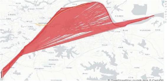
Figure 1 Different trajectory with same MMSI.

1 Introduction

AIS data is the primary data source of maritime supervision and traffic flow analysis [1–3]. The accuracy and reliability of data sources will directly affect the analysis results. However, the shortcomings of AIS equipment information being easily modified and signal transmission being greatly disturbed by the environment to cause the confusion of AIS original data, which exert a lot of negative effects on maritime supervision and ship safety. Among them, the most serious problem is that multiple ships share the same MMSI number. When this issue occurs, as shown in Figure 1, the normal trajectory on the screen is invisible in the mixed trajectory, which misleads the supervisor’s assessment and decision-making on the safety situation of the marine vessel, thus causing unnecessary collision risk [4, 5]. This issue has raised the attention of many scholars. In 2007, Harati-Mokhtari et al. [6] analyzed the reliability of AIS data, found the identity issue in AIS data, and summarized the common numbers and causes of such phenomena. Cutlip [7] pointed out that the ship MMSI problem existed in the fishing boat in the ocean may provide cover for illegal fishing behavior, thus avoiding the supervision of relevant departments. However, they have not put forward effective methods to solve such problems.

There are two main approaches to solving the identity problem. One is to filter the abnormal data as an abnormal value by setting the threshold, and the other is to separate these data as multiple trajectories. Most researchers adopt mature data cleaning technology in the field of database research. Wei et al. [8] studied the trajectory clustering method of AIS data. In the pre-processing process, the author found that there existed the same MMSI but different ship trajectory drift phenomena. In order to keep the data clean, the author chose to delete the trajectory directly. Obviously, the simple method of this kind of data will directly result in the loss and waste of data resources. Gao et al. [9] suggest that different ship trajectories with the same MMSI usually appear as z-beating, which is often mistaken as noise points in the data. Therefore, in the pre-processing, these offset points are usually filtered out by means of median or mean filtering, Kalman filtering, and example filtering. However, this method only maintains the integrity of a specific trajectory, rather than recovering multiple trajectories from it. Liu et al. [10] used AIS filtering and interpolation methods to clean abnormal data, so as to analyze the coverage of the Yangtze River inland AIS base station. Kraus et al. [11] firstly divides the trajectory according to the time threshold and performs anomaly data filtering on the chaos trajectory according to the speed threshold. This method can only get one of the trajectories, which results in the missing of other trajectory data. Either eliminating abnormal data or filtering it to get one of the trajectories will result in the loss and waste of AIS data resources, and there is no strict basis on how to determine a suitable threshold for data filtering. Mazzarella et al. [12] found that MMSI, like 0,1,123456789, was shared by many ships very common. Therefore, the author separates the ship’s trajectory point by point according to the dynamic information of the ship’s speed, time and angle. However, its data cleaning efficiency needs to be improved. Kodiyan et al. [13] analyzed a variety of data quality problems in movement data sets and proposed an algorithm to detect and repair data ID anomalies. Zhao et al. [14] analyses the main data quality problems existing in AIS, extracts the velocity difference and time difference from the trajectory points as characteristics and proposes a data cleaning framework based on separation, correlation and filtering for separating different ship trajectories sharing the same MMSI. However, in these methods, without considering the change of angle, the two close trajectories in the same period cannot be separated completely based on the difference of time and distance.

The core of separating AIS data of ships with the same MMSI is ship trajectory clustering. Zhu et al. [15] calculates and normalizes the distance matrix by considering velocity, angle, time and distance firstly. Then incremental DBSCAN method was applied to cluster the Inland Ship trajectories and analyze the behavior patterns of bifurcation channel inflow and upstream ferry. The disadvantage is that the selected trajectory sample is limited, which includes only some sections or seasonal data, so the analysis results can only represent the trajectory characteristics of a few ships. Zheng et al. [16] employs DBSCAN algorithm to cluster and merge berthing trajectory points under the framework of Hadoop. Compared with the commonly used stop/move model, the accuracy of this algorithm is improved by 20%. However, due to the limitation of ship type and data quantity of trajectory data and the rationality of DBSCAN parameter selection, some berth points cannot be identified. The trajectory clustering methods mentioned above are based on DBSCAN algorithm, which is poor to extract clusters with varying density. Yang et al. [17] uses TR-OPTICS algorithm to classify the trajectory points, improves the traditional OPTICS clustering algorithm, reduces the complexity of the algorithm and successfully realizes the taxi trajectory clustering.

The purpose of this paper is to collect, classify and recycle the different ships’ movement data with same MMSI as a recoverable data resource in the processing of AIS abnormal data, and to discuss and analyze the occurrence of major AIS issues in inland waterway traffic. Because the discovery and pre-processing of identity issues is a cyclic process, it requires the combination of model calculation and manual recognition. Visual analysis is a method of using human-computer interaction to combine data visualization technology with human visual cognition to obtain the wisdom behind the data. This method has been successfully applied in many fields, especially mobile data analysis and geographic information GIS systems [18–20]. The abnormal data processing is an iterative and iterative process. It needs to integrate automatic data processing technology and human subjective experience and knowledge to make a comprehensive judgment.

At first, this paper introduces the different ships with the same MMSI phenomenon and the causes of its occurrence. Secondly, the application of the optics-based spatiotemporal clustering method in separating the AIS chaos trajectory is illustrated. Then the overall analysis process and the specific functions of each visualization model and their interaction means are explained. Finally, the clustering algorithm and visual analysis method are empirically tested based on real river traffic flow data and typical case analysis. The results show that the combination of the spatiotemporal clustering method and the visual analysis method based on optics is feasible in the analysis of AIS abnormal data. Our main contributions are in two aspects. On one hand, a visual analytics method interacting with OPTICS algorithm was presented to deal with the identity issue of AIS data. On the other hand, the major situation of ship identity issues existing in inland waterway was discussed and resolved by examples to evaluate the AIS data quality.

2 Optics Method

The optics clustering algorithm is an improvement on the well-known DBSCAN algorithm and an extension of DBSCAN. The algorithm outputs a cluster structure of results sorted by the reachable distance, which makes it insensitive to the radius $ε$ .

2.1 Definition

Based on the definition of DBSCAN, the OPTICS method introduces two definitions needed by the algorithm: the core distance is the distance between the core point and its MinPts point (Equation (1)).

In the aspect of the core point $p$ , the reachable distance of $o$ to $p$ is defined as the maximum value of the distance from $o$ to $p$ and the core distance of $p$ (Equation (2)):

${core-dist}_{ε, M i n P t s}$
$= {\begin{matrix} UNDEFINED & if \| N_{ε} (p) \| < M i n P t s \\ MinPts -th smallest distance to N_{ε} (p) & otherwise \end{matrix}$	(1)
${reachability-dist}_{ε, M i n P t s} (o, p)$
$= {\begin{matrix} UNDEFINED & if \| N_{ε} (p) \| < M i n P t s \\ \max ({core-dist}_{ε, M i n P t s} (p), dist (p, o)) & otherwise \end{matrix}$	(2)

2.2 Procedures

The procedures of the algorithm are shown as follow:

X: The points to be clustered.
Q: cluster structure is sorted by reachable distance and the point with the smallest reachable distance is at the head of the team.
O: Result queue, the ordered queue as final output.
Input: sample set X, neighborhood parameters ( $ε$ , MinPts), the basic flow is:
(1) Initialize the core object set $Ω = \emptyset$
(2) Traverse the elements of X, if it is a core object, add it to the core object set $Ω$
(3) If the elements in the core object set $Ω$ have been processed, the algorithm ends, otherwise go to step 4.
(4) In the core object set $Ω$ , an unprocessed core object o is randomly select. Firstly, o marked as processed, and push it into the ordered list p, finally, the points that are unprocessed in the $ε$ -neighborhood of o are sequentially stored in the seeds set due to the reachable distance which is calculated according to timestamp, longitude, latitude and course.
(5) If the seed collection seeds $=$ $\emptyset$ , jump to step 3, otherwise, the closest seed point is picked from the seed collection seeds, mark it as visited and the seed as processed. Then the seed is pushed in the ordered list p and determines whether the seed is the core object. If yes, the unprocessed neighbor points are added to the seed collection and recalculate the reachable distance. Finally, the reachable distance is calculated with respect to the seed point and jumps to step 5.

After the ordered result queue is obtained by the above algorithm, the peaks and bottoms in the ordered queue are observed from cluster structure graph. In addition, the trajectories are clustered in the next step.

3 Design and Interaction of Visualization System

3.1 Analysis Framework

In the framework of collaborative visual analysis of abnormal data, as shown in Figure 2, users first exchange and filter the trajectory points of different regions in the map to explore the data of interest, and then cluster the data into OSM maps. Then, the results of cluster structure are drawn and the appropriate threshold is judged manually to separate mixed trajectories. Finally, different trajectories are tagged and stored in the database.

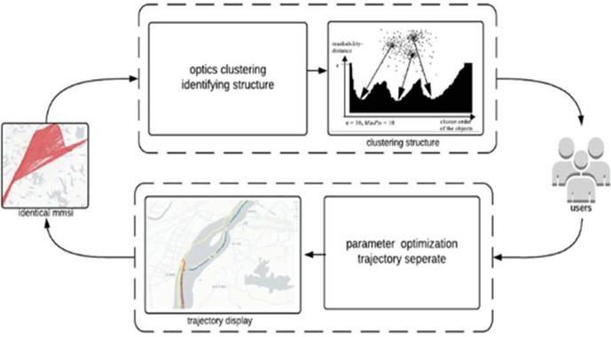
Figure 2 Analysis workflow.

3.2 Analysis Interface

The interface of the system consists of four parts, including parameter widget for optimizing parameter by visualization shown in the map, timeline visualization for displaying the detail information of sub-trajectory, cluster structure for determining parameter threshold and OSM, as shown in Figure 3. The OSM is an open platform that provides the basic map editing component and supports common trajectory point display operations. Additionally, users are free to draw points, lines and other data based on their data content.

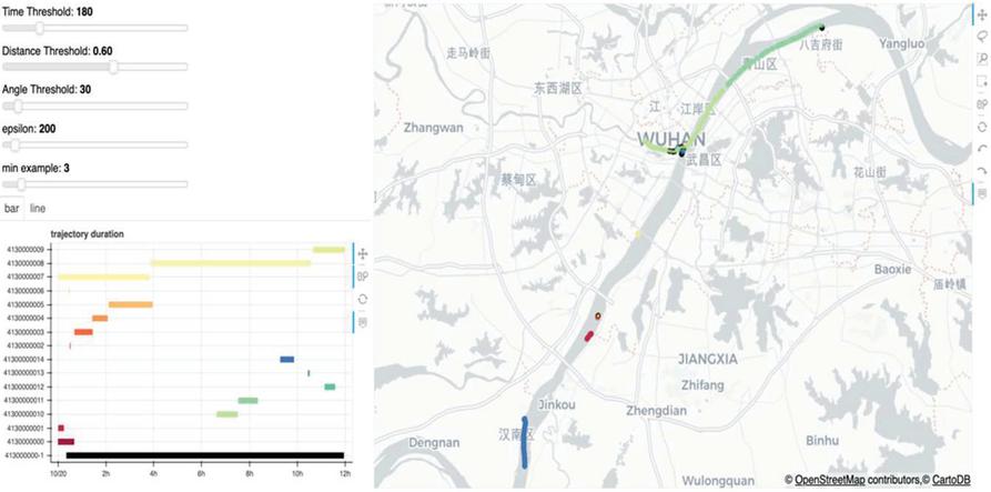
Figure 3 Analysis interface.

3.3 Analysis Interface

3.3.1 Map interaction

Apart from the basic operations such as zooming in, zooming out, and panning, the tool of OSM map includes lasso selection, box selection, and box enlargement. The lasso selection can be more convenient to filter the trajectory with any shape. As shown in Figure 4, Especially when multiple trajectories gather densely, it is flexible to use lasso selection to choose interesting tracks or points.

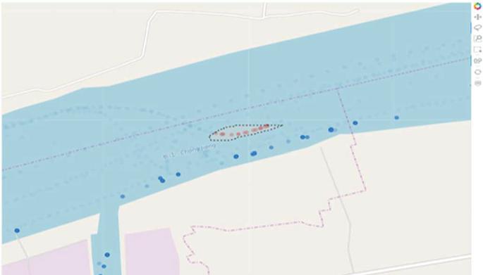
Figure 4 Selection on Map.

Figure 5 Cluster structure.

3.3.2 OPTICS parameter interaction

As mention in the above chapters, the optics algorithm calculates a cluster structure sorted by reachable distance. As shown in Figure 5, a curve graph is draw which regards firstly sorted reachable distances as the horizontal axis, and the distance value as the vertical axis. By observing the peaks and bottoms in the graph, the slider is adjusted to modify the optics parameter thresholds, in which epsilon denotes the distance value in vertical axis and min example refers to the minimum samples should be contained in one cluster. Then the cluster of different trajectory points is illustrated in OSM. Finally, the separation of different trajectories is realizing according to observation of the different visualization shown in map caused by algorithm optimization.

3.3.3 Sub-trajectory display and interaction

In the visualization of ship trajectory, the temporal correlation between trajectories is also an important clue to analyze ship behavior. The timeline model is used to display and interact with the separated trajectories. The time of the trajectory is displayed, and the time elapsed, so as to discover the correlation of the time series between the trajectories. When users interested in a sub-track in the map, they can select the prompt tool to hover mouse over the corresponding color and MMSI track bar to display the specific information of the track. As shown in Figure 6, the start and end time of the sub-track are shown as a text label.

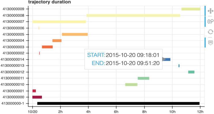
Figure 6 Sub-Trajectory information.

4 Case Study

The data in this paper is selected from the AIS base station of the Yangtze River Maritime Bureau in the AIS database. The main research areas are Nanjing, Wuhan and other inland river bridge areas. The main research objects are different ships with MMSI 413000000, 123456789. Among them, AIS data mainly contains the dynamic information, including the latitude and longitude, timestamp, speed and angle of the ship’s position and the static information, including the ship’s MMSI, the ship’s name and the number of the receiving base station.

After the cluster structure is obtained from the above data by adopting the OPTICS algorithm, the peaks and bottoms can be figured out clearly. Through the slider widget, clusters of different density can be obtained by selecting an appropriate threshold, so as to achieve the purpose of separating the mixed trajectory. In below, different situations will be discussed by dividing trajectory points into two categories: dynamic and static trajectory points.

4.1 Separation Between Dynamic Trajectory Points

4.1.1 Trajectory with similar direction

The similar direction trajectory refers to the trajectory of the vessels move in the same direction. When such trajectories share the same MMSI, they usually appear as a zigzag trajectory, as shown in Figure 7, which leads to visual disturbance to the analyst.

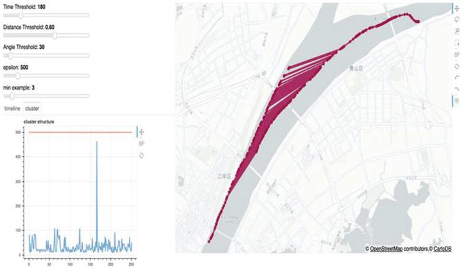
Figure 7 Mixed Trajectory with similar direction.

According to the peak and bottom in cluster structure shown in the lower-left corner, it can be observed that a prominent peak divides all trajectory points into two categories. When epsilon chooses between 110 and 460, the trajectory points belonged to two ships can be separated shown in Figure 8.

Figure 8 Trajectory after separation.

It can be figured out from the timeline model (Figure 9) that there is an overlap between the two separated tracks in the time axis, so sharing the same MMSI will present a zigzag shape.

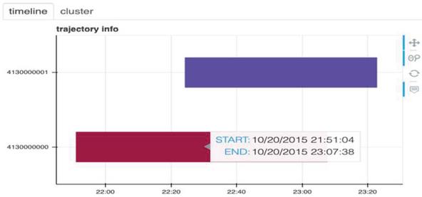
Figure 9 Sub-trajectory information display.

When the two tracks are close in time and space, even cross together, as shown in Figure 10.

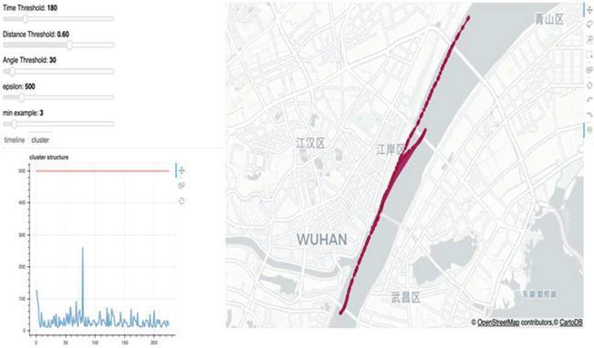
Figure 10 Cross trajectory.

It is still useful even in the case of Cross Trajectory. From the cluster structure, it can be observed that there are two clusters exist in the graph. When epsilon is chosen to be 200, the mixed trajectories are entirely separated to form two overlapping tracks shown in Figure 11.

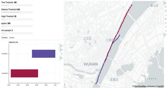
Figure 11 Trajectory after separation.

4.1.2 Trajectory with opposite direction

The opposite trajectories are also a common situation in chaos trajectory. Since in this type of chaos trajectory, the ships are constantly approaching and then successively moving away. Thus an x-shaped trajectory is produced as shown in Figure 12.

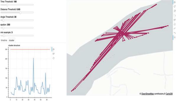
Figure 12 Mixed trajectory with opposite direction.

The separation method is the same as above. Firstly, by observing the graph of clustering structure, the threshold of reachable distance is found. Then the parameter epsilon is selected as 150. The separation effect of the two trajectories corresponding to the parameter is shown in Figure 13.

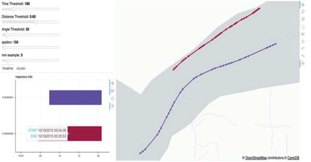
Figure 13 Trajectory after separation.

4.2 Separation Between Static Trajectory Points

There are many wharves in the inland waterway built for passengers and cargo ships. When the ship is staying at the wharf, a large amount of AIS data will still be generated due to the continued power supply. When two ships with the same MMSI appear, they will also cause a mixed trajectory shown in Figure 14. In order to separate such trajectory, the static trajectory points need to be extracted by a filter with a speed of 0 at the first. Then multiple complete ship trajectories are selected as the primary research objects.

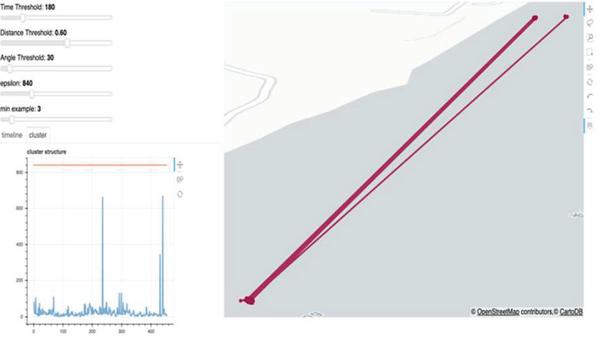
Figure 14 Mixed trajectory with static points.

According to the above cluster structure, the stay points can be divided into three classes when epsilon between 380 and 600. The separation effect is shown as Figure 15 when epsilon is 400. The results show that it is feasible in the separation of different stay points with same MMSI.

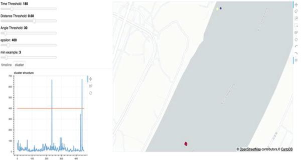
Figure 15 Trajectory after separation.

4.3 Separation Between Static and Dynamic Trajectory Points

By the above methods, the clustering and separation between static and dynamic trajectory points were respectively realized. Since the motion trajectories and the stationary trajectories usually exist in the inland waters at the same time, a fan-shaped trajectory is formed as shown in Figure 16 when the two situations occur simultaneously and the ships’ MMSI is identical.

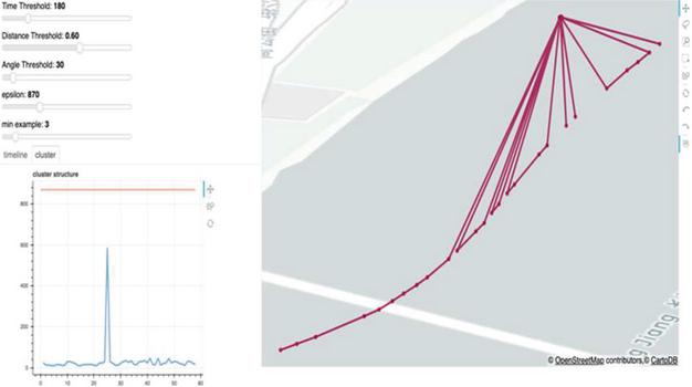
Figure 16 Trajectory mixed with dynamic and static points.

It is evident that there is a peak in the cluster structure, so it can be judged that when the parameter is between 100 and 600, the track points can be divided into two categories, as shown in Figure 17. The corresponding trajectory is divided into a stationary trajectory and a motion trajectory when the parameter is selected as 370.

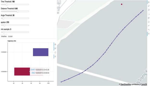
Figure 17 Trajectory after separation.

5 Conclusion and Future Work

In order to solve the problems existing in data filtering methods commonly applied in data pre-processing of different ships shared one MMSI in the inland waterway and ocean, this paper proposes a visual analysis method based on OSM map and OPTICS clustering for mixed trajectory separation. In the case study of the Wuhan section of the Yangtze River, the separation of the mixed trajectories under different situations is realized by discussing and analyzing the different situations between the static points and the moving points. The experimental results show that the visual analysis is effective in trajectories with identity issues. In the current study, when dealing with chaos trajectory, a single fixed threshold cannot be fully applied, and sometimes there is a case of excessive separation which is required further aggregation operations. In the future work, more visualization models will be added to display the separated trajectory data in a diversified way.

Acknowledgements

This work is supported by the Fujian Province Natural Science Foundation (Nos. 2018J01506, 2020J01860), and University-industry cooperation program of Department of Science and Technology of Fujian Province (No. 2019H6018) and The Key Project of Science and Technology of Wuhan (No. 201701021010132).

References

[1] Li M, Mou J, Liu RR, et al. Relational Model of Accidents and Vessel Traffic using AIS Data and GIS: A Case Study of the Western Port of Shenzhen City [J]. Journal of Marine Science and Engineering, 2019, 7(6): 163.

[2] Scheepens R, Hurter C, Van De Wetering H, et al. Visualization, selection, and analysis of traffic flows [J]. IEEE transactions on visualization and computer graphics, 2015, 22(1): 379–388.

[3] He W, Zhong C, Sotelo MA, et al. Shortterm vessel traffic flow forecasting by using an improved Kalman model [J]. Cluster Computing, 2017: 1–10.

[4] Claramunt C, Ray C, Salmon L, et al. Maritime data integration and analysis: recent progress and research challenges [J]. Advances in Database Technology-EDBT, 2017, 2017: 192–197.

[5] Chen C, Wu Q, Gao S. Quality assessment model for shipping data sources of the Yangtze River [C]//2017 4th International Conference on Transportation Information and Safety (ICTIS). IEEE, 2017: 355–361.

[6] Harati-Mokhtari A, Wall A, Brooks P, et al. Automatic Identification System (AIS): data reliability and human error implications [J]. The Journal of Navigation, 2007, 60(3): 373–389.

[7] Kimbra, Cutlip. “Spoofing: One Identity Shared by Multiple Vessels.” Global Fishing Watch. Web. 25 July. 2015.

[8] Wei Zhaokun. The vessels trajectory clustering and its applications based on AIS [D]. Dalian Maritime University, 2015

[9] Gao Qiang, Zhang Feng-Li, Wang Rui-Jin. Trajectory Big Data: A Review of Key Technologies in Data Pro-cessing [J]. Journal of Software, 2017, 28(4): 959–992.

[10] Liu L, Liu X, Chu X, et al. Coverage effectiveness analysis of AIS base station: a case study in Yangtze River [C]//2017 4th International Conference on Transportation Information and Safety (ICTIS). IEEE, 2017: 178–183.

[11] Kraus P, Mohrdieck C, Schwenker F. Ship classification based on trajectory data with machine learning methods [C]//2018 19th International Radar Symposium (IRS). IEEE, 2018: 1–10.

[12] Mazzarella F, Alessandrini A, Greidanus H, et al. Data fusion for wide-area maritime surveillance [C]//Workshop on Moving objects at Sea. 2013.

[13] Kodiyan NJ. Detection and correction of mover identity problems in movement datasets [D]. The Technical University of Munich. 2018.

[14] Zhao L, Shi G, Yang J. Ship trajectories pre-processing based on AIS data [J]. The Journal of Navigation, 2018, 71(5): 1210–1230.

[15] Zhu Jiao, Liu Jingxian, Chen Xiao, et al. Behavior Pattern Mining of Inland Vessels Based on Trajectories [J]. Journal of Transport Information and Safety, 2017, 35(3): 107–116.

[16] Zheng Zhentao, Zhao Zhuofeng, Wang Guiling. Ship trajectory extraction method for port stop area identification [J]. Journal of Computer Applications, 2017, 28(4): 959–992.

[17] Yang Shuliang, Bi Shuoben, Athanase Nkunzimana, et al. Spatial clustering method for taxi passenger trajectory. Computer Engineering and Applications, 2018, 54(14): 249–255.

[18] Lei Jinyu, Chu Xiumin, He Wei, et al. Visual Analytic System of Vessel Traffic in Bridge Waterway [J]. Journal of Shanghai Jiao Tong University, 2017, 51(7): 840–845.

[19] He Zhao-cheng, Zhou Ya-qiang, Yu Zhi. Regional traffic state evaluation method based on data visualization [J]. Journal of Traffic and Transportation Engineering, 2016, 16(1): 133–140.

[20] Andrienko G, Andrienko N, Fuchs G. Understanding movement data quality [J]. Journal of location Based services, 2016, 10(1): 31–46.

Biographies

Jinyu Lei received his Ph.D. in Transportation Engineering from Wuhan University of Technology, China. Currently he is a lecture with Minjiang University, China. His research interests include visual analytics, maritime situation awareness, and artificial intelligence with its application in transportation safety.

Xiumin Chu received his Ph.D. in Automotive Engineering from Jilin University, China. Currently he is a professor with National Engineering Research Center of Water Transport Safety, Wuhan university of technology, China. His research interests include safety control in waterway transportation, information collection and processing in traffic engineering, and intelligent waterway transportation.

Wei He received his Ph.D. in Transportation Engineering from Wuhan University of Technology, China. Currently he is an associate professor with Minjiang University, China. His research interests include data analysis and mining, traffic control and management, and artificial intelligence with its application in transportation safety.