Geospatially Partitioning Public Transit Networks for Open Data Publishing

Harm Delva, Julián Andrés Rojas, Pieter Colpaert and Ruben Verborgh

IDLab, Department of Electronics and Information Systems,

Ghent University – imec, Ghent, Belgium

E-mail: harm.delva@ugent.be; pieter.colpaert@ugent.be

*Corresponding Author

Received 15 December 2020; Accepted 29 March 2021; Publication 24 June 2021

Abstract

Public transit operators often publish their open data in a data dump, but developers with limited computational resources may not have the means to process all this data efficiently. In our prior work we have shown that geospatially partitioning an operator’s network can improve query times for client-side route planning applications by a factor of 2.4. However, it remains unclear whether this works for all network types, or other kinds of applications. To answer these questions, we must evaluate the same method on more networks and analyze the effect of geospatial partitioning on each network separately. In this paper we process three networks in Belgium: (i) the national railways, (ii) the regional operator in Flanders, and (iii) the network of the city of Brussels, using both real and artificially generated query sets. Our findings show that on the regional network, we can make query processing 4 times more efficient, but we could not improve the performance over the city network by more than 12%. Both the network’s topography, and to a lesser extent how users interact with the network, determine how suitable the network is for partitioning. Thus, we come to a negative answer to our question: our method does not work equally well for all networks. Moreover, since the network’s topography is the main determining factor, we expect this finding to apply to other graph-based geospatial data, as well as other Link Traversal-based applications.

Keywords: Linked data, open data, mobility, maintainability, web API engineering.

1 Introduction

Open Data can lower the barrier to entry for new players to enter existing markets, leading to more available applications for end-users. A direct result of this is that niche markets can be serviced, and Return of Investments are higher, since initial investments are relatively low. The OpenStreetMap data for example can be used to build very specific route planning applications, such as a cycling route planning for the city of Brussels¹ or a route planner for motorcyclists that want scenic and curvy roads.² Public transit data is a noteworthy success story of Open Data, in large part due to the General Transit Feed Specification (GTFS): the preferred data format of the Google Transit APIs, which many people interact with through Google Maps. This is an example of a rising tide lifting all boats; most operators just want to get their data into the Google APIs, but the same data can be used by others for any use case.

However, these GTFS datasets are not without their faults. While a GTFS feed of London’s public transit network is only 100 MB large after gzip compression, processing this data can require over 26 GB of memory.³ Such memory requirements make the data unwieldy to use in common environments such as entry-level cloud computing services. Moreover, not all operators respect the standard data model, and many have started providing non-standard data files. The Belgian railway operator for instance includes a file named stop_times_overrides.txt,⁴ but the meaning of this file is undocumented. Other operators do document their extensions,⁵ but all these extensions have fragmented the ecosystem at the cost of the data users.

Publishers of Open Data often follow the Linked Data principles [1], as the latter’s usage of the Resource Description Framework (RDF) can be a partial solution to the data interoperability problem. One of the principles of Linked Data is that URIs are used to identify resources, and these resources can then be accessed through the Web for more information [1]. People and autonomous agents alike, can keep following such links to get at least a basic understanding of the data’s semantics. In other words, Linked Data does not solve the interoperability problem; but it brings the problem into focus and presents data publishers and consumers with a common framework to work with heterogeneous data.

The Linked Connections specification [2] proposes a Linked Data alternative to GTFS data dumps, in which the public transit connections are published as a paginated collection, and each page contains data from a certain time interval. Applications that need only need data from a specific interval to answer a query can thus be more selective in the data they have to process. In our own prior work [3], we explored the option of fragmenting this geospatially, by the stops’ physical location as well as the connections’ departure time. We have shown that this can improve the query time performance of client-side route planning applications by a factor of 2.4, and that the method used to fragment the network itself is less important than the fragmentation’s granularity. However, it remained to be investigated what this means for other public transit networks, or other kinds of geospatial data in general. In this paper we aim to provide more general insights into why and how geospatial partitioning works and discuss what this entails for other use cases and other kinds of data.

2 Related Work

We identify four domains of related work which we discuss in the following subsections: (i) research in the field of Linked Data and how the Semantic Web has focused on making data reusable and interoperable, (ii) Linked Traversal Querying and how it uses Linked Data to solve queries (iii) contemporary mobility data specifications, and (iv) how public transit networks are currently being partitioned and for what purpose.

Throughout this paper we use three similar, but different, terms: cluster, partition, and fragment. When operating on a discrete set of objects, the difference between clustering and partitioning is one of perspective; clustering combines similar items while partitioning starts from the set of all items – so that clustering individual public transit stops partitions the network itself. A planar space, such as the world, can also be partitioned, in which case the partitions are often referred to as cells or regions. A Fragment on the other hand stems from the field of Linked Data and refers to Linked Data Fragments, which are resources on the Web.

2.1 Linked Data Fragments

To facilitate interoperability with other datasets, Open Data is often Linked Data as well. Tim Berners-Lee outlined the four principles of Linked Data [1]: (i) use URIs as names for things, (ii) use HTTP URIs so that people can look up those names, (iii) when someone looks up a URI, provide useful information using standards such as RDF [4], and (iv) include links to other URIs so that they can discover more things. In the conceptual framework of Linked Data Fragments [5], this is just one interface to access Linked Data. Data can also be published as a large data dump, or through a querying API on top of the raw data. What all these interfaces have in common is that they expose a fragment of the entire dataset, so that they can all be considered Linked Data Fragments, with data dumps and query APIs on the two extremes on the Linked Data Fragments axis [4]. This axis illustrates the trade-offs between different methods of publishing Linked Data on the Web. Data dumps put the data processing burden on the client’s side but allow the most flexibility for clients. Query APIs on the other hand put the processing burden on the server side but always restrict, in some way, the way the data can be used.

All Linked Data Fragments contain a set of controls: functions which can be used to discover other fragments. In the case of a data dump this set of controls will often be empty as there are no other fragments, whereas the set of controls of a query API is the API endpoint itself. Fragments elsewhere on the axis often contain hypermedia controls, which describe how, as well as for what purpose, other fragments can be used. Vocabularies such as Hydra [6] and TREE⁶ can be used to describe these controls as RDF triples. The former of which contains constructs such as paginated collections, access controls for resources, and URI templating. The TREE vocabulary focuses on paginated collections by adding qualifiers such as numeric values to the links. These qualifiers can be used to describe ordered collections, or searchable indexes.

2.2 Link Traversal Querying

Data found on the Web is traditionally replicated into centralized databases, so that the data can be indexed prior to opening it up to querying. Both the indices and the replicated data need to be kept in sync with the original data set, which can make such systems burdensome to maintain. Link Traversal Querying [7] is an alternative approach, where the query processor operators under the “follow-your-nose” principle of Linked Data. These processors traditionally operate without prior knowledge of the data [8]: they only know what they discover through following links on the Web. In other words, there is no replicated data set to keep in sync – all information is ephemeral. Query performance is in large part determined by the number of links that are traversed to come to an answer [9], making link prioritization a crucial feature of these query processors. We will use an instance of a Link Travel Query Processor later in this paper, to evaluate the behavior of the various public transit networks.

2.3 Mobility Data

The General Transit Feed Specification (GTFS) is, at the time of writing, the de facto standard for publishing public transit schedules. A single feed is a combination of 6 to 13 CSV files, compressed into a single ZIP archive. Its core data elements are stops, routes, trips, and stop times. Stops are places where vehicles pick up or drop off riders, routes are two or more stops that form a public transit line, trips correspond to a physical vehicle that follows a route during a specific period, and stop times indicate when a trip passes by a stop. This data is not only useful for route planning applications, but other applications also include embedding timetables in mobile applications, data visualization; accessibility analysis, and planning analysis [5].

The Linked Connections specification [2] defines a way to publish transit data that falls somewhere in the middle of the Linked Data Fragments axis. Connections are defined as vehicles going from one stop to another without an intermediate halt. These connections are then ordered by departure time, fragmented into documents, and are then published on the Web. Data consumers can use the semantics embedded in each fragment to solve their own queries. This, combined with the fact that each fragment is easily cacheable, make Linked Connections servers more scalable than full-fledged route planning services. Linked Connections fragments contain two kinds of hypermedia controls: a search template is defined for the collection as a whole, and every fragment links to the next and previous fragments. The search templates can be used by clients for accessing a specific point in time directly, while the pagination links are used for traversing a time interval.

2.4 Partitioning Public Transit Networks

Researchers in the field of route planning have noted that methods based on partitioning have been successful for accelerating queries on road networks, but that adapting those methods to public transit networks is hard [6, 7]. One of the main differences is that road networks are topological networks. Public transit networks on the other hand are also inherently time dependent. On top of that, it is not even clear what exactly needs to be partitioned as different algorithms can require wildly different data models [8].

The Scalable Transfer Patterns [9] algorithm aims to reduce preprocessing times of the original Transfer Patterns [10] algorithm. The authors compared 4 different techniques to partition stops into clusters of equal size: (1) k-means using the stops’ geographical locations, (2) a merge-based clustering with a utility function that punishes big partitions and rewards pairs of partitions with high edge weights between them, (3) a general-purpose graph clustering algorithm called METIS [11], and (4) a road partitioning method called PUNCH [12]. They found that k-means, despite being completely oblivious to the network structure outperformed both METIS and PUNCH while their own merge-based approach performed the best of all. HypRAPTOR [8] is another route planning algorithm that uses METIS to partition the network graph, but which uses clusters of trips instead of stops.

2.5 Prior Work

In our own prior work [3] we investigated what data publishers can do to make their open transit data easier to use. We used four different clustering methods to partition a single public transit network and evaluated each method’s effect on the query performance of a client-side route planning application. Voronoi diagrams were used to convert clusters of stops to geospatial partitions, whose boundaries were then described using the GeoSPARQL vocabulary [15]. Finally, the TREE vocabulary was used to create an index of partition-specific Linked Connection resources.

Our results showed that a small number of partitions combined with a simple method such as k-means is a good practical choice, as more granular partitions or complicated methods yield diminishing returns. However, we were left with few generalizable as it is still unclear whether the same method works equally well on other types of public transit networks, other kinds of geospatial data, or other kinds of data applications. In this work we aim to verify our original findings on the same network we used initially, as well evaluate the same method on two different networks.

Figure 1 On the left is a heatmap that visualizes the arrival locations of all connections on the Flemish regional transit network on Tuesday November 3 $^{r d}$ 2020. Visualized on the right is a heatmap of the passenger’s destinations, based on one week of anonymized query logs given to us by the operator themselves. Note that there are places with a considerable number of connections that are in low demand, especially in the West of the region.

3 Method

Geospatial data represents our physical world and under the assumption that people are most interested in their own surroundings, we posit that public transit data contains some sort of locality bias, i.e., data related to certain regions is in higher demand than data from most other regions. Looking at Figure 1, we see this bias manifest itself in two ways: public transit connections are more frequent in urbanized areas, and users of public transit networks favor 3 areas above all others (from left to right: the cities of Ghent, Antwerp, and Leuven). The Linked Connections publishing scheme enables applications to access data at a specific point in time, but each data fragment still contains data from the entire transit operator’s service area. Our own prior work has shown that geospatially partitioning this specific network improves the query performance of client-side route planners, and we now investigate how this translates to other networks and other applications.

3.1 Data Sources

We partition three public networks in Belgium: the national railways (NMBS/SNCB), the regional operator in the region of Flanders (De Lijn), and the network of the city of Brussels (STIB-MIVB). Table 1 shows a summary of the evaluated networks’ characteristics. For the sake of simplicity, we assume each network’s operating area matches its designated administrative area. The number of daily connections was measured on Tuesday November 3rd 2020, and we will keep using data from this day throughout the remainder of this paper.

Table 1 The national railway network is physically the largest, but also contains the least amount of data. The regional network on the other hand contains the most data, but the average stop has only 31 passages per day – compared to 97 passages per day on the national railway. The average stop on the city network is the busiest with 121 passages per day and is also by far the densest at 17 stops per km $^{2}$

Network	Area (km $^{2}$ )	Stops	Daily Connections	Size (MB)
National	30,689	677	65,837	13
Regional	13,625	36,425	1,139,335	1,910
City	162	2,675	323,941	346

3.2 Partitioning

Most existing work focuses on clustering stops, or trips, into discrete sets of objects. If a data publisher were to follow this approach, they would have to explicitly assign a label to every new stop the data owner adds. Failing to do so would cause them to publish incomplete data, as unlabeled stops will not be in any published cluster. Instead, we chose to partition the physical world instead of creating discrete sets of stops. The resulting partitions are then described semantically and published over the Web, allowing any agent to infer to which cluster every stop belongs. In other words, data publishers do not have to explicitly label every stop themselves – the data speaks for itself. Both data publishers and consumers perform this same reasoning step when encountering a new stop, so that all involved actors are at all times synchronized with each other.

We start by adapting two clustering methods that are often used to partition transit networks: k-means and METIS. However, both methods disregard one important feature of transit networks: k-means does not consider network connectivity and METIS does not consider physical locations. This leads us to design an additional method, called Hub, which clusters stops by their proximity to important transportation hubs. As others have shown good results from hierarchical methods, we also consider a merge-based adaption of Hub, which we name Merge. Each method is used to generate a geospatial partitioning, which divides the physical, continuous world into a set of non-overlapping regions, often referred to as cells.

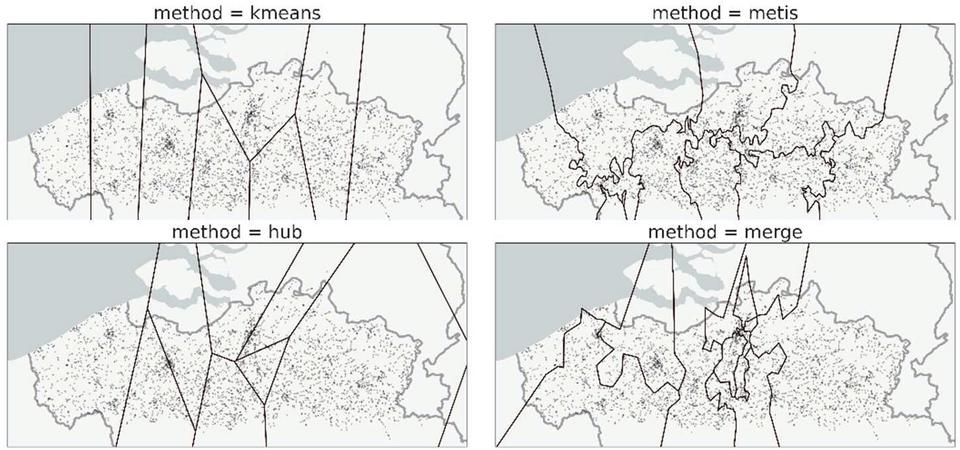
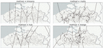
Figure 2 The 8 partitions each evaluated method creates on the regional transit network. Note that the two methods on the top row create regions of roughly equal sizes, while the approaches at the bottom create regions of varying sizes. The approaches in the left column create regions with simple shapes, while the ones on the right create irregular shapes. The Merge method even creates the illusion that more than 8 partitions are generated, as some are only held together by a thin sliver.

3.2.1 K-means

Existing work has found k-means to be competitive with more complex methods [9], so it should be considered among the state of the art for this use-case. As the name implies, this algorithm distributes a given set of points in exactly k clusters, where every point belongs to cluster with the nearest cluster mean. Iterative heuristics exist to compute this clustering, and we used the implementation from scikit.learn⁷ with default parameters, using the stops’ WGS84 coordinates as input.

To obtain a spatial partitioning from this, we create a Voronoi diagram using the cluster means as seed points. Because the Voronoi cells of two adjacent points on the convex hull share an infinitely long edge, we add some extra padding points that represent the bounding box of the operator’s service area – and then discard all infinite edges.

3.2.2 METIS

METIS is another algorithm that is used to partition public transit networks [8] [9] and is among the state of the art of graph clustering algorithms. We follow the conventional approach of creating a vertex for every stop and connecting them with an edge if they are connected through a single connection. Every edge is assigned a weight that corresponds to how many connections connect those stops. We used a Python wrapper⁸ of the reference implementation to compute the clustering, using the contig option to force contiguous partitions.

The METIS algorithm only sees the network as a connectivity graph though – it does not consider the physical location of the stops. This means that even though it creates contiguous clusters, those clusters are not contiguous in the physical world. We obtain a clean spatial partitioning using an additional post-processing step that (1) creates the Voronoi diagram of all stops, (2) merges all Voronoi cells that belong to the same cluster, and (3) merge isolated areas into the surrounding cluster.

3.2.3 Hub

Hub is our own method that aims to incorporate both the geospatial and the graph-like nature of public transit networks. It iteratively selects the stops based on which trips pass through it. In the first iteration it selects the stop with the most unique trips, in the subsequent iterations it selects the stop with the most unique trips that the previous stop(s) do not have. After k iterations it contains the k most important hubs, which lead us to name this method Hub. These selected stops are then used as seed points to create a Voronoi diagram. To illustrate the simplicity of this approach, Listing 1 contains all the necessary code, up until the creation of the Voronoi diagram.

images

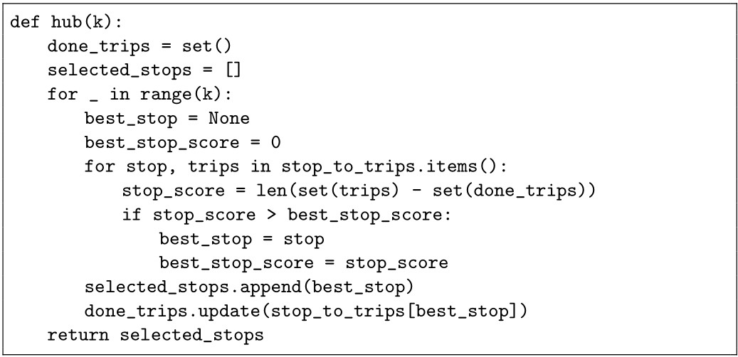
Listing 1 The Hub method implemented in just 14 lines of Python code.

3.2.4 Merge

Instead of stopping the Hub algorithm after k iterations we can also let it terminate, and then use the symmetric difference to merge the two most similar adjacent Voronoi regions until only k remain. As there is a finite number of trips, this algorithm has a clear termination condition: it stops when all trips are covered by one of the selected stops. This makes the process more complex, but existing work has shown good results using hierarchical clustering techniques [9]. We have named this approach Merge, as it is a merge-based variation of the Hub method.

images

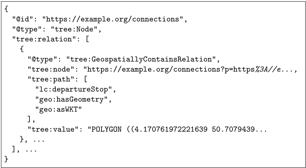
Listing 2 Excerpt of a JSON-LD representation of a view index. The tree:node property points to a hydra:PartialCollectionView, which is a connections page from the original Linked Connections specification. The tree:value property defines which geospatial area that view covers, while the tree:path property defines which property of the connections should be compared to this geospatial area.

3.3 Hypermedia Controls

Hypermedia plays an essential role in how data consumers discover, and interact with, resources on the Web. Especially in the case of Linked Data Fragments resources, as hypermedia controls are the glue that link individual fragments together. In the case of a regular Linked Connections data source, consumers access the data by either filling in a Hydra [13] search template, or by starting from any time fragment and following links until they find all required data. The existence of this search template can in turn be discovered by reading a fragment’s hypermedia controls, or it can be contained in a data catalogue. In the case of our partitioned data set, the server creates one view per partition, and then creates an index of all generated views. We express all geospatial data as Well Known Text (WKT) literals, as provided by the GeoSPARQL vocabulary [14]. The TREE vocabulary⁹ is then used to link to each generated view, including the view’s geospatial extent as qualifier to this link. Listing 1 contains an excerpt of such an index but note that it also states that each view contains connections whose departure stop lies in this region. Without this information, it would still be unclear to data consumers how these views can be used, e.g., one might assume incorrectly that a view contains all connections crossing its geospatial extent.

4 Evaluation

We evaluate the effectiveness of geospatially partitioning public transit network on the use case of a client-side route planner. Such an application lies at the intersection of route planning – the most common use case for mobility data – and Link Traversal Querying. We use an adapted implementation of the Connection Scan Algorithm [19], in which case the traversed links correspond to public transit connections. We consider a simplified scenario of route planning where the queries consist of 3 values: (i) a departure stop, (ii) a destination stop, and (iii) a departure time, and where the expected result is a route with the earliest possible arrival time. Initially, only the departure stop is known to be reachable at the specified departure time, the reachability of all other stops is discovered by following connections. Route planning starts with following the first connection that starts at the departure stop after the specified departure time. At this point two stops are known to be reachable at a certain time, and the process continues by following the next connection that starts at either of the reachable locations, and this continues until the destination stop is reached. To obtain realistic results, we also consider that travelers can walk between stops at a constant speed of 5 km/h.

We partitioned the three different public transit networks described in Section 3.1, using data from a single day – November 3rd 2020 – as input for the clustering algorithms. Each algorithm is used to create 4, 8, 16, and 32 clusters. A redis-backed server stores an ordered list of all connections within every generated region and exposes these using the hypermedia controls described in Section 3.3. The same server also hosts a version of the data with one cluster that contains all the data, i.e., without any geospatial partitioning. Altogether we test 51 different configurations (4 partitionings for each of the 4 methods, and the baseline for each of the 3 networks), and each data fragment contains 20 minutes of data.

For the regional public transit operator, we randomly selected 2000 queries from logs given to us by the operator itself, and likewise we selected 2000 queries for the national railway network from the publicly available iRail logs¹⁰. We were unable to obtain realistic queries for the city network, so we generate an artificial dataset by uniformly sampling departure and arrival stops from the list of existing stops. The departure times were likewise generated by uniformly sampling the query set of the regional network operator – under the assumption that the rush hours on both networks are similar. Finally, to measure the impact of the locality bias, we generated artificial query sets for the regional and national networks as well.

We aim to eliminate as many variables as possible to isolate the impact of the partitioning itself; the client and server run on two separate machines on the same local network, a constant 20 ms of latency is added to each response, and the client only processes one query at a time. As is fitting for an evaluation of client-side route planning, the client ran on a consumer-grade laptop which contains an Intel i7-8650U CPU, clocked at 1.90 GHz, and 16 GB of memory. All evaluation code, resources, and results are available through a publicly available Git repository.¹¹ Only the Linked Connections data itself is excluded due to file size restrictions, but the code to download these assets manually is included instead.

5 Results

We start by examining the baseline to gain some insights into how the baseline behaves, as well as what the differences are between the query set that was generated from real query logs and the artificial ones, we generated ourselves. Table 2 shows a large discrepancy between each evaluated network; whereas the average query time is only 0.6 s on the national railway network, this number increases to 26 s on the regional transit network. We also see the first piece of evidence of the locality bias in realistic route planning queries. Both the query times and distances are, on average, twice as large on the artificial query sets compared to the real ones.

Table 2 The mean query time and the physical distance between the departure and destination stops when using the original Linked Connections data, i.e., the baseline. Note the large standard deviations in the query times, but more so in the real query sets as these queries are skewed towards shorter journeys

Network	Query Set	Query Time (s)	Query Distance (km)
National	Real	0.6 $\pm$ 0.3	35.3 $\pm$ 23.1
	Artificial	1.2 $\pm$ 0.4	66.4 $\pm$ 39.7
Regional	Real	26.0 $\pm$ 21.4	20.5 $\pm$ 18.8
	Artificial	38.0 $\pm$ 17.6	43.3 $\pm$ 22.8
City	Artificial	2.9 $\pm$ 1.2	5.8 $\pm$ 2.9

5.1 Query Performance

Using geospatially fragmented data entails that clients must process less unnecessary data, so an improvement in query performance, i.e., the time it takes to answer a given query, is to be expected. However, this improvement is modest as there will always be a minimal amount of data that needs to be processed to answer a query. In other words, the large variation of query times as shown in Table 2 remains. To facilitate one-to-one comparisons, we measure the improvement relative to the baseline instead.

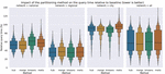
We use envelope plots [16] to visualize the results, as these plots show the median value as a black line, as well as the 75%, 87.5%, … quantiles as separate boxes. These additional statistics are not to be overlooked when interpreting the visualizations, as they show that some configurations have a tighter distribution than others, and that some have a more skewed distribution.

Figure 3 k-means is the least consistent of all evaluated methods, as it shows the worst results on the national railway network but the best results on the city network. Neither method does well on the city network however, with the median speedups ranging from 10% to 12%. Note that in 25% of the queries on the city network, METIS had a negative effect on the query performance.

In our prior work we concluded that the choice of partitioning method is less impactful than we initially expected, although the methods that resulted in simple boundaries had a slight edge. As we now expand our evaluation to other networks, we notice that this is not entirely true. Figure 3 shows that k-means, which we initially saw as the most practically viable option, is outperformed by the other evaluated methods. Although k-means performs well on the city and the regional networks, where the stops are distributed uniformly throughout the network, its effectiveness on the national railway network is noticeably worse. A visual inspection reveals that k-means can create empty partitions, as it gets skewed by irregularly visited international stations. For example, when creating just 4 partitions, one partition corresponds to the country of France – even though very few trains operated by the Belgian railways visit those stops. Indeed, k-means is the only evaluated method that does not consider the connection frequency. METIS shows the second worst results, especially in the worst case, and this method also considers only one dimension of the data: the connection frequency. Of the other two methods, merge is the most promising, which implies that simple partitions boundaries are less important than we initially believed. However, our results do confirm that the chosen method has minor impact. The median improvement using the Merge method – over all networks and all granularities – is 83%, while k-means results in a 66% improvement as well.

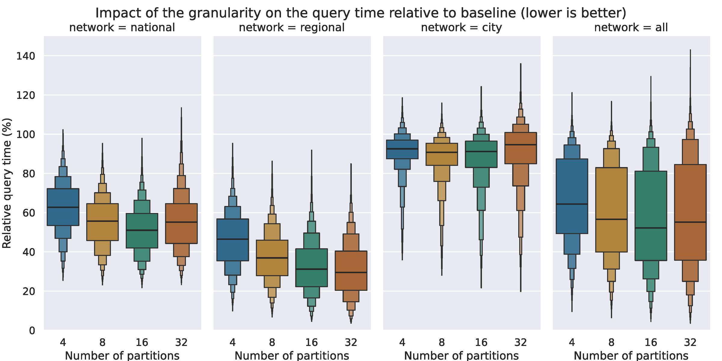
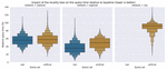
Figure 4 More granular partitions yields diminishing returns, as there is a minimal amount of data that needs to be processed to answer a query, while the computational overhead of adding more partitions does keep increasing. The optimal granularity depends on the network though; whereas 16 partitions show the best results on the national railway network, whereas the optimum for the regional network is closer to 32 – or beyond.

The partitioning granularity on the other hand is more impactful, although Figure 4 shows this again varies from network to network. Using 4 partitions is enough to reduce the query times on the regional network by 54%, and 32 partitions even results in a 70% reduction. Again, we see less improvements on the city network, where using 8 partitions yields the best results: a 10% improvement on the average query. When combining the results from both real query sets, i.e., from the regional and national networks, using 16 partitions reduces query times by 59%, or by 57% when using 32 partitions.

The lesser improvements on the city network could be due to the artificially generated query set, or it could be due to a characteristic of the network itself. As mentioned in Section 4, we have also generated artificial query sets for the other two networks. If the difference is entirely caused by the locality bias present in the real query sets, we would expect to see little to no improvements on the artificial query sets on the other networks as well. As Figure 5 shows, this is not the case. Even with the artificial query set, we see a signifcant improvement on both the regional and national network although the improvements are smaller than with the real query sets. The difference between the two query sets is particularly small on the national network – but a t-test reassures us that the difference is statistically significant (P $<$ 0.001). Altogether, this shows that the locality bias of a query set does have an impact on the potential speedups, but that there is more at play.

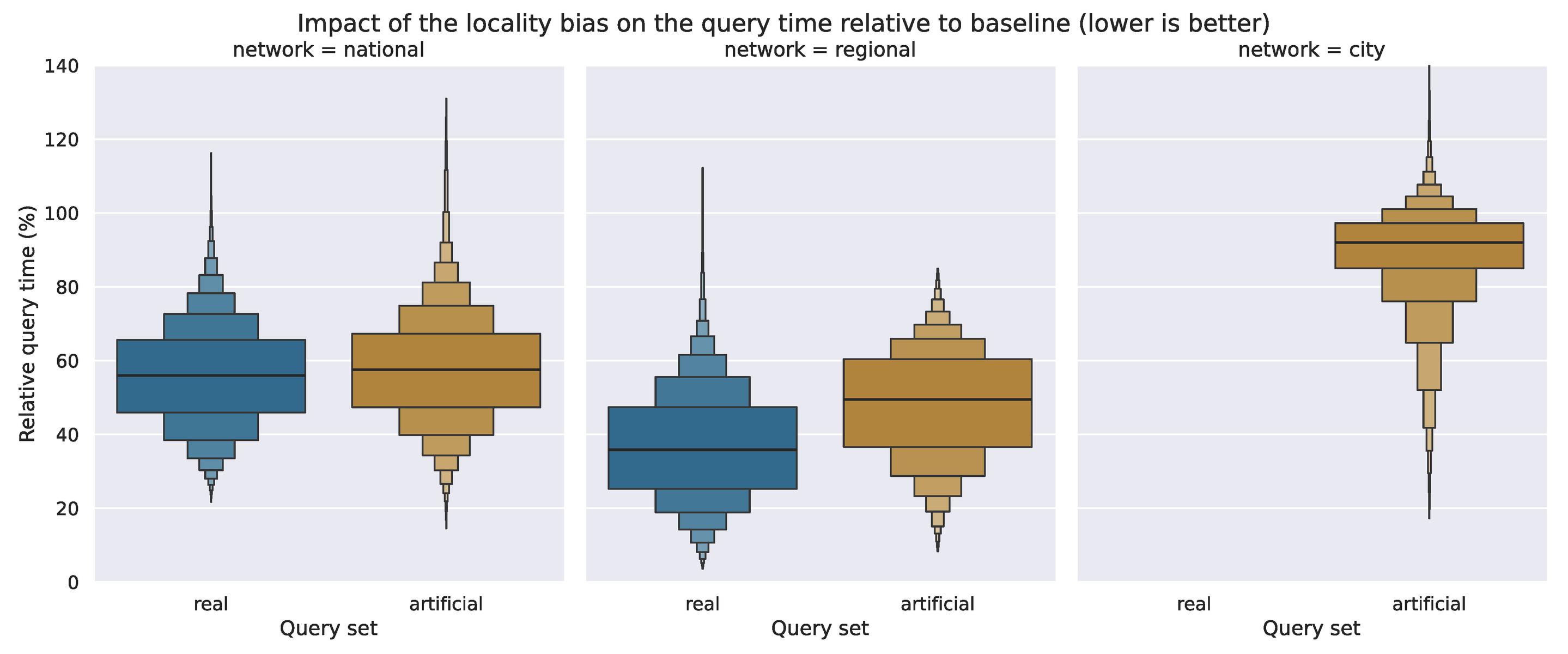
Figure 5 The improvements on the national network are nearly the same as when using the artificial query set, where query times are reduced by 42%, whereas the real query set sees a 43% improvement. On the regional network on the other hand, we only see a 46% improvement when using the artificial query set, compared to 63% when using the real query set. In any case, the improvements on both networks are significantly better than on the city network.

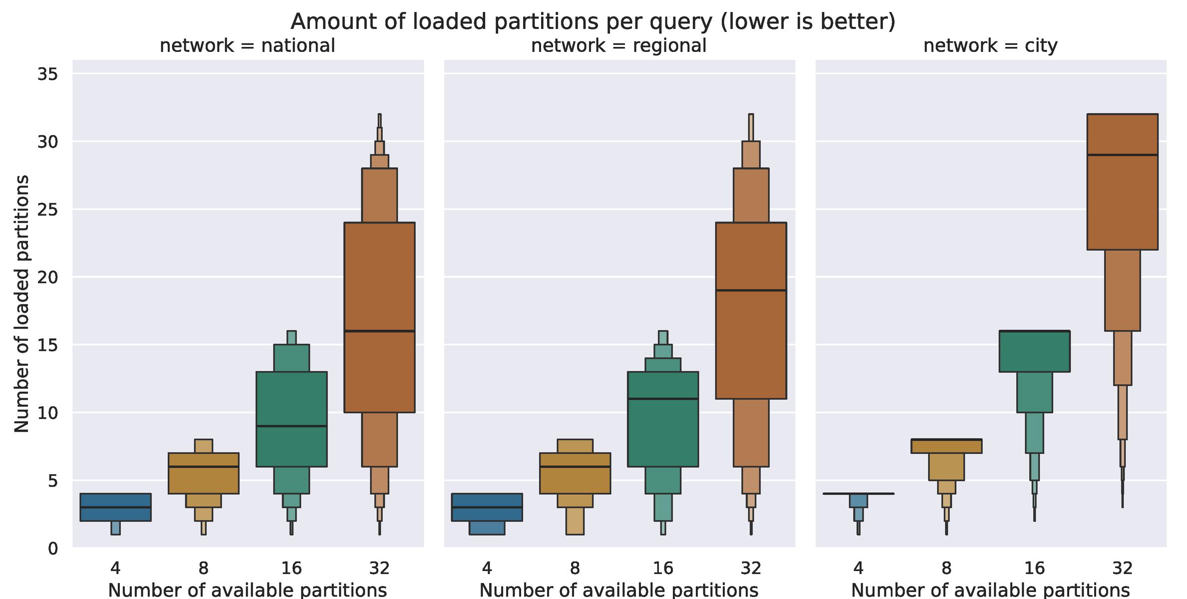
Figure 6 Up until a granularity of 32 partitions, the average query on the city network uses all available partitions. Using the artificially generated query sets of the other networks, the average query only requires half of all available.

Indeed, Figure 6 shows that when processing the artificial query sets on the regional and national networks that the average query can still be solved using half the available partitions, whereas the average query on the city network use all available partitions – except at a granularity of 32, when 29 partitions are used in the average case. Staying with the artificial query sets of all networks, we also evaluate how many of the networks’ stops are reached on average. Table 3 shows that seems to be the determining factor; the average query on the city network visits 72% of all stops in the network – twice the fraction of visited stops on the other networks. This may be a side effect of our optimistic usage of transfers on the routes – as we assume a constant walking speed of 5 km/h. However, the average speed when crossing the city network is still 10 km/h, while the average speed through the regional network is only 7 km/h. In other words, the network connectivity in the city network is not a direct result of the transfers – leaving the network topography itself as the most logical cause.

Table 3 The travel time, distance between departure and destination stops, and the percentage of stops reached by the average artificial query on each network

Network	Travel Time (Hour)	Query Distance (km)	Stops Reached (%)
National	3.6 $\pm$ 2.6	66.4 $\pm$ 39.7	36
Regional	5.9 $\pm$ 2.9	43.3 $\pm$ 22.8	33
City	0.6 $\pm$ 0.3	5.8 $\pm$ 2.9	72

5.2 Cache Behavior

Caching is an important aspect of Linked Connections, and Linked Data Fragments APIs in general, as the caching ensures the scalability of these APIs. As we are making the data more fine-grained, we must measure the effect this has on the overall caching behavior. Caching can happen at multiple points in the network, but since we use anonymized query logs, we cannot know which requests were done by the which clients. Instead, we focus exclusively on server-side caching, and assume all requests are done by distinct clients.

While running the query performance evaluations, we also record which resources are requested. These requests are then replicated and run through a simulated LRU cache to measure the hit rates. We set the cache size to 2% of what would be required to keep the entire dataset in memory. These caches are smaller than what would be used in a real setting, but this does make the differences between the configurations more apparent. Figure 7 shows that the cache hit rates do indeed drop quickly as the partitions become more granular. Indeed, the most granular partitioning would place every stop in its own partition, at which point it devolves into a standard REST API. However, even with 32 partitions the warm cache hit rates hover around 10%, which is largely due to the rush hour that is present in all evaluated query sets. We again see the difference between the national and regional networks, where we have access to a real query set with some locality bias, and the city network.

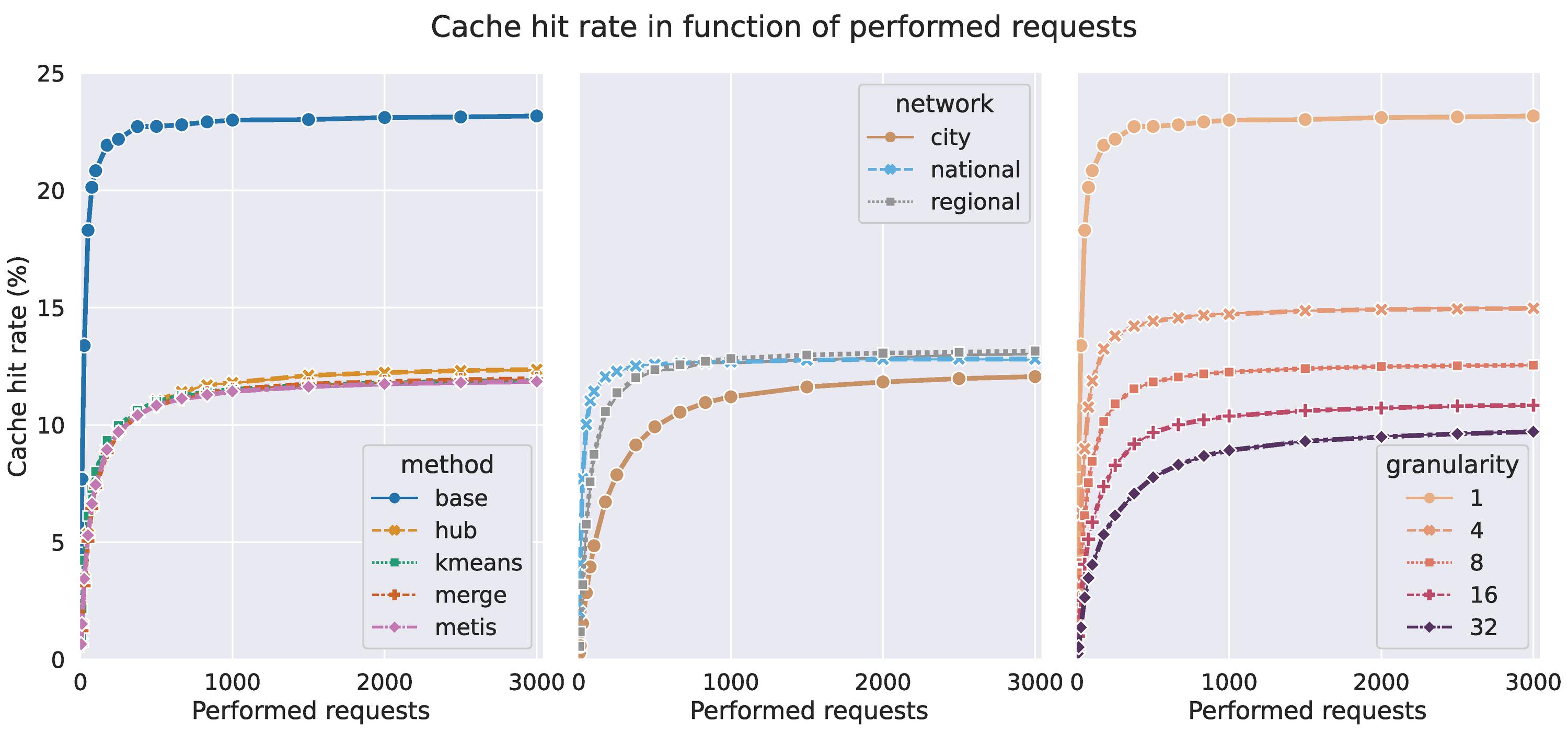
Figure 7 From left to right, we see that the unpartitioned baseline data achieves a warm cache hit rate of 23%, while the average hit rate of the partitioned data lies around 12%. In line with the query performance results, the national railway network and regional network yield better results. Finally, the difference between no partitioning at all and 4 partitions is larger ( $-$ 8%) than the drop from 4 partitions to 32 partitions ( $-$ 5%).

6 Discussion

On the regional public transit network, we came to mostly the same conclusions as in our prior work; all evaluated methods reduce query times by 62%. The national railway network sees smaller, but still comparable improvements. However, we did not succeed in making queries on the city network reliably faster, with 25% of the evaluated queries becoming slower with the partitioned data.

When seen as an instance of Link Traversal Querying, client-side route planning applications still follow the exact links regardless of the geospatial partitioning. As a result, the expected improvement is limited to reducing the amount of parsed unnecessary data – and there is little such data when querying over the dense city network as 72% of all available stops are by the average query. In other words, the intrinsic characteristics of this network of this network make it hard to partition efficiently.

Another determining factor is how people utilize the network itself, as it is easier to effectively partition a network if the average traveler only visits specific sectors of the network. We verified this by generating artificial query sets where the average query is equally likely to visit any stop in the network and found that this does indeed diminish the improvements. However, even with the artificial query sets, we see a 46% and 42% improvement on respectively the regional and national networks – indicating that network characteristics are more influential.

We also invalidate some findings of our own prior work, as increasing the partition granularity does make it harder to efficiently cache the data. Geospatially partitioned data is easier to cache if certain areas if certain partitions are requested more often, but routes often traverse otherwise unpopular regions. As a result, all partitions in between popular partitions become popular as well. When all partitions are in high demand, the available cache space cannot be used any more efficiently than with unpartitioned data. On the contrary, as the data becomes more granular, we see more cache misses as the API devolves in a standard REST API.

7 Conclusion

In this paper we investigated what data publishers can do to make their open transit data easier to use. Based on research from the field of route planning, we explored the idea of geospatially partitioning public transit networks. We evaluated 4 different clustering methods for the use-case of client-side route planning: k-means, METIS, and two domain-specific methods of our own. The partitions were obtained using Voronoi diagrams and were then published with the appropriate hypermedia controls that clients can use to discover clusters of public transit stops. As in our prior work, we see that the specific partitioning method has minor impact on the results, and that the partition granularity is more impactful.

We set out to learn whether this approach works equally well for various kinds of public transit networks, and the answer to this question is negative. Specifically, a dense city network proves hard to partition effectively, as the average evaluated query visits 72% of all available stops – implying that this network is too connected. We expect that this insight applies to other kinds of graph-like geospatial datasets, and future research could explore the relation between established graph metrics and the graph’s suitability for geospatial partitioning. Finally, we wanted to know whether these insights translate to other use cases as well, or if they are limited to the specific case of client-side route planning. If strongly connected graphs are simply ill-suited to geospatial partitioning, this would translate directly to other link-travel based applications.

Notes

¹https://routeplanner.bike.brussels

²https://kurviger.de/en

³https://github.com/opentripplanner/OpenTripPlanner/issues/2063

⁴https://data.gov.be/nl/node/62230

⁵https://gtfs.org/extensions/

⁶https://treecg.github.io/specification/

⁷https://scikit-learn.org/0.20/modules/clustering.html#k-means

⁸https://metis.readthedocs.io/en/latest/

⁹https://treecg.github.io/specification/

¹⁰https://gtfs.irail.be/logs/

¹¹https://github.com/hdelva/jwe_paper_results

References

[1] T. Berners-Lee, “Linked data-design issues,” 2006. [Online]. Available: https://www.w3.org/DesignIssues/LinkedData.html.

[2] P. Colpaert, A. Llaves, R. Verborgh, O. Corcho, E. Mannens and R. Van de Walle, “Intermodal public transit routing using Liked Connections,” in International Semantic Web Conference: Posters and Demos, 2015.

[3] H. Delva, J. A. Rojas, P.-J. Vandenberghe, P. Colpaert and R. Verborgh, “Geospatial Partitioning of Open Transit Data.,” in International Conference on Web Engineering, Helsinki, 2020.

[4] E. Miller, “An introduction to the resource description framework,” Bulletin of the American Society for Information Science and Technology, vol. 25, pp. 15–19, 1998.

[5] R. Verborgh, O. Hartig, B. De Meester, G. Haesendonck, L. De Vocht, M. Vander Sande, R. Cyganiak, P. Colpaert, E. Mannens and R. Van de Walle, “Querying datasets on the web with high availability,” in International Semantic Web Conference, 2014.

[6] M. Lanthaler and C. Gutl, “Hydra: A Vocabulary for Hypermedia-Driven Web APIs.,” LDOW, vol. 996, 2013.

[7] O. Hartig, C. Bizer and J.-C. Freytag, “Executing SPARQL queries over the web of linked data,” in International Semantic Web Conference, 2009.

[8] O. Hartig, “Zero-knowledge query planning for an iterator implementation of link traversal based query execution,” in Extended Semantic Web Conference, 2011.

[9] O. Hartig and M. T. Ozsu, Walking without a map: optimizing response times of traversal-based linked data queries, 2016.

[10] A. Antrim and S. J. Barbeau, “The many uses of GTFS data - opening the door to transit and multimodal applications,” Location-Aware Information Systems Laboratory at the University of South Florida, 2013.

[11] A. Berger, D. Delling, A. Gebhardt and M. Müller-Hannemann, “Accelerating time-dependent multi-criteria timetable information is harder than expected,” in 9th Workshop on Algorithmic Approaches for Transportation Modeling, Optimization, and Systems (ATMOS’09), 2009.

[12] R. Bauer, D. Delling and D. Wagner, “Experimental study of speed up techniques for timetable information systems,” Networks, 2011.

[13] D. Delling, J. Dibbelt, T. Pajor and T. Zündorf, “Faster transit routing by hyper partitioning,” in 17th Workshop on Algorithmic Approaches for Transportation Modelling, Optimization, and Systems (ATMOS 2017), 2017.

[14] H. Bast, M. Hertel and S. Storandt, “Scalable transfer patterns,” in 2016 Proceedings of the Eighteenth Workshop on Algorithm Engineering and Experiments (ALENEX), 2016.

[15] H. Bast, E. Carlsson, A. Eigenwillig, R. Geisberger, C. Harrelson, V. Raychev and F. Viger, “Fast routing in very large public transportation networks using transfer patterns,” in European Symposium on Algorithms, 2010.

[16] G. Karypis and V. Kumar, “A fast and high quality multilevel scheme for partitioning irregular graphs,” SIAM Journal on scientific Computing, vol. 20, pp. 359–392, 1998.

[17] D. Delling, A. V. Goldberg, I. Razenshteyn and R. F. Werneck, “Graph partitioning with natural cuts,” in 2011 IEEE International Parallel & Distributed Processing Symposium, 2011.

[18] R. Battle and D. Kolas, “Geosparql: enabling a geospatial semantic web,” Semantic Web Journal, vol. 3, pp. 355–370, 2011.

[19] J. Dibbelt, T. Pajor, B. Strasser and D. Wagner, “Connection Scan Algorithm,” 2017.

[20] H. H. Wickham, K. Kafadar and Hadley, “Letter-value plots: Boxplots for large data,” 2011.

Biographies

Harm Delva. He is a PhD student at IDLab, affiliated with both Ghent University and imec. My original research subject lay at the intersection of the Semantic Web technologies and Linked Open Data publishing, but with a focus on researching how applications can find and use this data – beyond the traditional SPARQL usecase. You can find more information on hdelva.be.

Julián Andrés Rojas. He got his MSc on Telematics Engineering from University of Cauca, Colombia in 2014. He started his PhD at Ghent University – imec in Pieter Colpaert’s team in 2017 on Linked Data publishing and querying on the Web. As part of his research, he has investigated the design and performance of Web interfaces for cost-efficient publishing and querying of Linked Open Data. Julián has applied his research and participated on projects about decentralized data sharing ecosystems in different domains such as public transit route planning, bicycle infrastructure, railway infrastructure and scientific research. Julián is author of several peer-reviewed publications presented in recognized venues such as ISWC, ESWC, TheWebConference and ICWE.

Pieter Colpaert. He is a post-doctoral researcher at IDLab – Ghent University – imec working on cost-efficient and maintable Linked Data Web APIs. Together with his team he applies this to different domains such as transport and mobility, cultural heritage, base registries, governmental data, environmental sensor data, or scholarly communication. He co-founded Open Knowledge Belgium, and is still a voluntary board member there, to fight for a world where knowledge creates power for the many, and not the few.

Ruben Verborgh. He is a professor of Decentralized Web technology at IDLab, Ghent University – imec, and a research affiliate at the Decentralized Information Group of CSAIL at MIT. He is also a technology advocate for Inrupt, supporting the Solid ecosystem that gives you back control and choice-online and offline. He loves discussing about the Web, Linked Data, decentralization, Web APIs, hypermedia clients, and much more.