An Algorithm with Efficiently Collecting and Aggregating Data for Wireless Sensor Networks
Peng Xiong1 and Qinggang Su2,*
1School of Electronics and Information, Shang hai Dianji University, Shanghai, China
2Chinesisch-Deutsche Kolleg für Intelligente Produktion, Shanghai Dianji University, Shanghai, China
E-mail: xiongp@sdju.edu.cn; suqg@sdju.edu.cn
*Corresponding Author
Received 22 January 2021; Accepted 03 February 2021; Publication 28 May 2021
Abstract
Due to the resource constraint, in wireless sensor network, the node processing ability, wireless bandwidth and battery capacity and other resources are scarcer. For improving the energy efficient and extend the lifetime of the network, this paper proposes a novel algorithm with the distributed and energy-efficient for collecting and aggregating data of wireless sensor network. In the proposed protocol, nodes can autonomously compete for the cluster head based on its own residual energy and the signal strength of its neighbouring nodes. To reduce the energy overhead of cluster head nodes, with a multi-hop way among cluster heads, the collected data from cluster heads is sent to a designated cluster head so as to further send these data to a base station. For improving the performance of the proposed protocol, a new cluster coverage method is proposed to fit the proposed protocol so that when the node density increases, network lifetime can be increased linearly as the number of nodes is increased. Simulations experiments show that network lifetime adopting the proposed protocol is sharply increased. And, the proposed protocol makes all the nodes die (network lifetime is defined as the death of last one node) in the last 40 rounds so that networks adopting the proposed protocol have higher reliability than networks adopting compared protocols.
Keywords: Collecting data, aggregating data, minimum spanning tree, cluster.
1 Introduction
With the development of new technology in the field of electronics and communications, a micro-wireless sensor with sense, wireless communication and data processing capability has been used widely. Because of the low-cost and low-power attributes, these sensors can are organized into wireless sensor networks (WSN) to monitor and sense a variety of environmental information (such as temperature, humidity, etc.). Today, WSN with a lot of micro-sensor and efficient-antenna nodes has become an important calculating platform [1–5].
Unlike the wireless mobile ad hoc networks (MANET), WSN typically has greater node’s density and weaker node’s mobility (generally, the nodes are no longer moved after being deployed) [6–8]. And due to the cost and size constraints, the sensor node processing ability, wireless bandwidth and battery capacity and other resources are scarcer. In particular, in many applications, because the deployment environment constraints, the node’s energy cannot be added, which makes how to extend the lifetime of the sensor network has become one of the key factors to be considered in the design of WSN. There have been a lot of research works to extend the lifetime of WSN [9–16] from different aspects. For the aspect of communication protocols, this paper presents a data collection and aggregation protocol with the efficient energy.
2 Related Work
The main task of WSN is to send the collected data from a general node to a base station (BS or The Sink). The simplest way to achieve this task is to send directly [17–21], that is, every node in network directly sends its collected data to BS. But, for those sensor nodes away from the base station, the energy overhead using for sending the data is very high so as to cause the sensor nodes to die soon. To solve this problem, some of the energy-saving algorithms have been proposed [22–26].
The reference [22] presented famous LEACH algorithm. It is a distributed and self-organized protocol. Its core idea is to reduce the number of nodes directly communicating with a base station to achieve the purpose of saving energy. The protocol uses rounds as a unit, each round is divided into two phases: cluster setup phase and stabilization phase. In the setup phase, with self-organized way, the cluster heads(CHs) are served by the nodes which are randomly selected. Then the selected cluster heads randomly broadcast, and the ordinary nodes join into the nearest cluster head according to the strength of the received signal to construct a cluster. In the stabilization phase, all members in the same cluster send the collected data to their CH so as to further aggregate and send them to BS. Since the cluster head must is randomly selected in each round, this algorithm can ensure that the energy overhead is uniformly distributed to all the nodes By data aggregation and the reduced number of nodes directly communicating with BS, compared with the others with the direct communication protocols, LEACH can extend the sensor network lifetime (the first node death) by 8 times. However, LEACH does not take into account the following: (1) The optimization of the number of CHs. In a sensor network, if the probability of a node becoming a CH in any round is p, then the number of cluster heads will increases proportionally with the number of nodes. (2) the way that CH communicates directly to BS can lead to higher energy overhead of the CHs away from BS; (3) The way of randomly selecting CHs causes the algorithm to not control the distribution of CHs in the network, while the distribution of CHs can determine the energy overhead of network in the current round.
Lindsey and Raghavendra research shows that in a certain distance range, the node transceiver consumes more energy than the node amplifying consumes. Based on it, they proposed PEGASIS protocol in the reference [23] so as to reduce the energy overhead of nodes. Its idea is to use greedy algorithm for all nodes in the network to construct one chain with the length sum of all edges close to the minimum, and each edge in the chain just receives or sends data once. Namely, in each round, a node receives data from a neighbour node located in the chain and aggregates these data with the existing data of the node so as to send them to another neighbour node in the chain. This sending and aggregating starts at the end node of the chain, along the chain, to the specified node, and then the specified node sends the final aggregated data to BS. Compared with LEACH protocol, PEGASIS has fewer the nodes to communicate directly to BS and has the stronger ability for aggregating data, which obviously reduces the energy overhead in each round. Especially when BS is far away from the monitored area, the effect is more obvious. However, for PEGASIS protocol, the network lifetime extending is under the condition that all nodes knew the global information of network, so it exists the following problems: (1) Due to the large scale of the sensor network and the node resource limitation, it is very difficult to save the globe information to a single node; (2) The reasons leading to the node failure is complex and varied, so maintaining global information requires a high cost; 3) PEGASIS protocol organizes all nodes in the network into one chain. If a node in the chain is dead, all data from the chain end node to this node is lost, so its fault-tolerant is poor (as shown in Figure 1, the node 4 is dead); (4) The length of the chain depends on the number of nodes, so there is a significant delay in the procedure of collecting data for a large WSN.
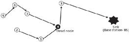
Figure 1 Illustration of PEGASIS protocol.
PEDAP protocol proposed in the reference [24] further developed PEGASIS protocol, the core idea of which is to construct all nodes of the sensor network into a minimum spanning tree. PEDAP protocol assumes that all nodes are isomorphic and the base station knows the location information of them in the network. Moreover, the base station can predict the remaining energy of any node in the network according to the node energy overhead which is certain in the radio communication model in each round. After a certain number of rounds, PEDAP protocol requires the base station to recalculate the routing information to exclude the dead nodes. When the calculation is complete, the base station sends its desired message, such as the father node of the node in the spanning tree and the time slot using for sending the data to its father node in each round, to each node. By this way, in the setup phase of PEDAP protocol, all nodes just need to receive messages from the base station, so the energy overhead in this phase is minimal compared with LEACH and PEGASIS protocols. However, when the reasons that the nodes is failure are not lack of energy (as shown in Figure 2, the node 4 is dead), PEDAP protocol is difficult to exclude the death nodes in time.
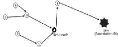
Figure 2 Illustration of PEDAP protocol.
As can be seen from the above analysis, if the algorithms based on the global or centralized scheme want to exclude the accidental death nodes, each node needs to periodically broadcast their own state, leading to the poor elasticity and a lot of energy overhead. The routing algorithm based on the cluster has good scalability and fault tolerance because of the property of the distributed and self-organization. The proposed protocol (ECAP) in this paper is just a data collection and aggregation protocol based on the cluster.
3 System Model and Problem Description
In line with the algorithms proposed in the reference [22–25], ECAP protocol is based on the cluster and uses round as unit. Each round consists of three stages: cluster generation, collection tree creation and data collection. They are respectively represented with T, T and T. Where T means the network monitoring stage in which the data from nodes is sent to BS to process. In order to ensure the effective working time, the algorithm must meet the formula T, T T.
3.1 The Network Model
In this paper, the sensor network with N nodes randomly and uniformly deploying in a rectangle area A abides by the following rules:
(1) Once deployed, all nodes are no longer moved. And the network does not require man-made maintenance.
(2) The location of BS that is outside the A is fixed, and BS is unique.
(3) All the nodes have similar ability (the processing / the communication) and are equal in status.
(4) The nodes are not equipped with GPS and cannot know its location by measuring.
(5) The nodes can adjust the transmit power according to the distance, that is, the wireless transmit power is controllable.
(6) The energy overhead of node in each round is not uniform.
The first three rules are typical settings in general sensor network. The fourth rule shows that ECAP protocol needn’t to use the location information of node. We think that when the system scale is increased, the number of exchanged message will be sharply grew, and the method determining the node location by exchanging message will lead the network efficiency to decrease. Furthermore, the energy overhead for exchanging message can also reduce the network lifetime. The fifth property mainly shows that from the aspect of the energy-saving, using different energy levels to send the messages from the intra-cluster communication and inter-cluster communication can significantly reduce the energy overhead of the nodes so as to extend the network lifetime. The sixth property shows that because the node energy overheads are different, ECAP must ensure that the energy overheads are uniformly shared by all the nodes.
3.2 Wireless Communication Model
In the past of years, there were many researches on low-energy wireless communication. ECAP uses the same wireless communication model as the reference [27]. In wireless communication model, a given threshold is d that is a constant depending on the environment. When the distance between the sending node and the receiving node is less than d, the energy using for transmitting data is in proportion to the square of this distance, or it is in proportion to the fourth power of this distance. And they correspond respectively to free space model and multipath fading models. Thereby, based on the distance between the sending node and the receiving node, the sending node may use different energy overhead models to get the energy for transmitting the data. Assuming that node a sends k bytes of data to node b outside distance d, then the energy overhead can be calculated using the following formula:
| (1) |
When b gets data from a, the energy overhead using for the wireless receiving device is as following:
| (2) |
Where the E denotes the energy overhead for the transceiver and the E denotes the energy overhead for the amplifier and its number depends on the distance between the sending node and the receiving node and the tolerable bit-error rate. Moreover, the most protocols and algorithms used data aggregating technologies to decrease the amount of sending and receiving data so as to save energy. ECAP protocol uses data aggregation technologies to reduce the energy overhead too. In line with PEGASIS protocol, ECAP assumes that the ability of data aggregation is , where A is an aggregating coefficient, N is the number of all nodes in the network and K is the packet size. The energy overhead for aggregating data is indicated in E. In addition, this paper assumes that the wireless channel is symmetric, that is, whether from the a to the b or from the b to the a, the energy overhead transmitting the message m is same.
3.3 Problem Description
Essentially, in the sensor network, in the case of minimizing the energy overhead of the system, the methods which use round as unit to extend the network lifetime can distribute the energy overhead uniformly to each node. For the cluster-based algorithm, the structure of the cluster will determine the energy overhead of system. Assuming that area A is randomly deployed with N nodes, this paper think that in order to decrease the energy overhead of system in each round and ensure that the energy overhead is uniformly distributed to each node, the cluster algorithm needs to meet the following requirements:
(1) The algorithm should be fully distributed and self-organization. And the node determines independently the self-state only according to the local information. Each node must determine whether to be a cluster head or a cluster member before the T ends.
(2) The energy overhead for communicating between the nodes should be as much as possible to meet the free space model, that is, the intra-cluster communication and inter-cluster communication need to meet the free space model. Since LEACH algorithm cannot ensure that the distribution of the cluster heads is ideal in the network, when the cluster head distribution is bad, the intra-cluster communication does not meet the free space model, leading to a large energy overhead as shown in Figure 3.
(3) The energy levels used for the inter-cluster communication and intra-cluster communication is different. In the case that the node density is sufficient, the coverage radius for communicating of the energy for the inter-cluster communication must is at least two times more than the cluster radius, and the network composed of all the CHs should be connectable.
(4) Optimizing the CH distribution. When the communication between the CHs meets the free space model, it is necessary to ensure that the interval between any two CHs is greater than the cluster radius r. In this paper, the r represents the size of cluster, that is, only those nodes with the distance away from a cluster head which is less than r can be allowed to join the cluster constructed by this CH. On account of the interference of the wireless channel, when the interval between the two CHs is less than r, it will aggravate the interference of the intra-cluster communication each other, leading to the unnecessary message retransmission so as to bring the extra energy overhead.
(5) The choice of the cluster head should take the residual energy of node into account. Unlike LEACH protocol, ECAP protocol does not assume that the energy overhead of cluster head is same in each round, so it is required to ensure that the energy overhead is uniformly distributed to each node so as to avoid the premature death of some nodes.
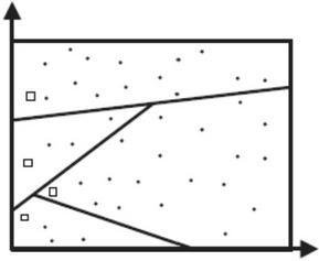
Figure 3 Illustration of the cluster distribution in LEACH protocol.
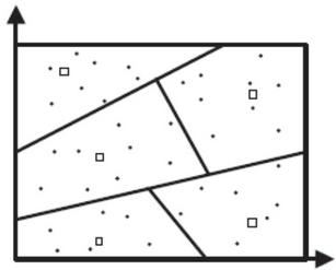
Figure 4 Illustration of the cluster distribution in ECAP protocol.
4 Protocol Description
ECAP protocol uses round as unit and is divided into three phases: T, T and T. In T, Once selected, the cluster head receives the messages from all the nodes which will join in the cluster constructed by this cluster head. And this cluster head creates a TDMA slot schedule and broadcasts the TDMA schedule to its member nodes. In order to further save energy, in T after T, CH is selected from all CHs as the unique node CH which can communicate with BS. And then the CH and the other cluster heads are respectively serve as the root node and the offspring nodes to create an approximate minimum spanning tree. In T, phase, the member nodes send the data to the cluster head according to the allocated time slot. After receiving the messages from all the offspring nodes in the spanning tree, the cluster head aggregates these data and sends them to its parent node. The above steps are repeated until the root node. And finally, the root node sends the aggregated data to the base station.
4.1 Cluster Generation Algorithm
In ECAP algorithm, the size of the cluster is fixed, and its radius r d/2. In order to ensure the connectivity between the cluster heads, ECAP defines that the communication radius R of cluster head must meet the formula R 2r, and the distance d between two neighboring cluster heads must meet the formula r d R. By these formula, the cluster heads in the sensor network will have an ideal distribution as shown in Figure 4. Since the size of the cluster is fixed and the relation among the clusters needs to meet the above constraints, in the monitored area A with the known size, the number of clusters required to cover A is directly depended on the size of A and the clusters. The reference [28] gives the formula to compute the minimum number of nodes required to cover A. In the formula (3), n represents the minimum number of nodes required to cover A.
| (3) |
Based on the formula (3), in order to restrict the number of the initial CHs, ECAP protocol defines the initial probability that any node S (1 i N) is to become a cluster head is as following.
| (4) |
Obviously, the final number of cluster heads: N Np. When ECAP protocol runs, in order to distribute uniformly the energy overhead to all the nodes, the probability p that a node becomes CH is related to its energy.
| (5) |
Where E is the current energy of node, and E is the initial energy of node. When the energy of node is less than a threshold E, it will no longer compete for CH. The lost energy using for sending, receiving and aggregating data can be predicted, so E can be calculated depending on the formula (6).
| (6) |
Where the “cycle” represents the number of times for collecting data in each round, and the “C” is the average number of members in a cluster, and the “l” is the size of packets.
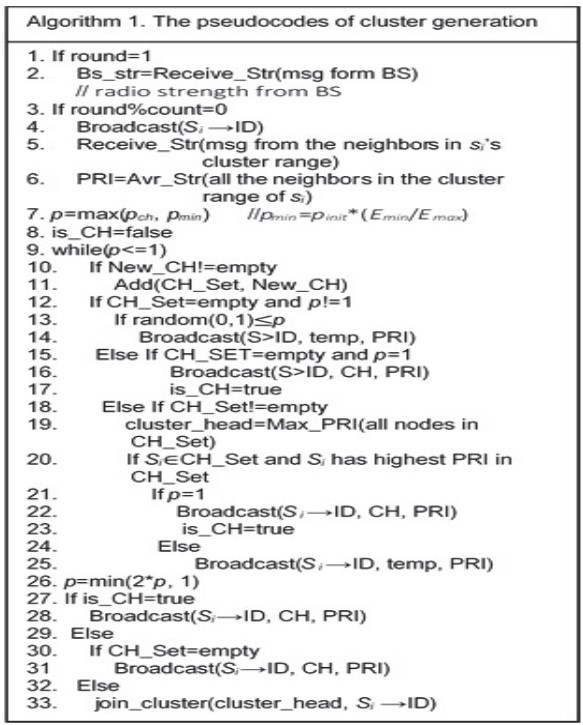
For any node S, in each round, the T must run the cluster generation algorithm. The main body of algorithm is some cycle codes, and the number of times for cycle depends on the E of node. The time of one cycle is t, the t should be sufficient to ensure that the S can receive the messages from all the nodes in a circular with the centre S and the radius r. Also, in order to extend the lifetime of the sensor network, when the node compete for CH, the energy is not the only factor to be considered. Before the start of cycle, S broadcasts within the scope of r and receives the data from the nodes within the same range. And then based on the received wireless signal intensity, let , where the m represents the quantity of neighbouring nodes in a circular with the radius r and the center S. The higher the PRI, the smaller the energy overhead of cluster with the cluster head S. So the PRI can be acted as a priority for node competing for CH. Since the node death (energy depletion) is predictable in the static sensor network, if the node has a small failure rate, the change of the neighbour set of each is little. Moreover, since ECAP protocol can distribute uniformly the energy overhead to each node so as to extend all nodes’ life in the network, it further increases the steady of the set of the neighboring nodes. It can be seen from the third line to the sixth line in the Algorithm 1 that in ECAP protocol, all nodes broadcast every count rounds to calculate the PRI, where the value of the count depends on the failure rate of node in the network.
At the beginning of each cycle, S first determines whether there is the broadcasts from a new cluster head, and if so, it adds the new cluster head to the candidate temporary cluster head set CH_Set. If the CH_Set is not empty and does not contain S, then S loses the opportunity as a cluster head. But if there is no the candidate cluster heads in the CH_Set announcing itself as a cluster head when a cycle is ended, then S doesn’t considers it is in any cluster and announces itself as a cluster head. If S is a candidate cluster head (S CH_Set), when a cycle is ended and the priority of S is also highest, then S announces itself as a cluster head. Otherwise, when a cycle is ended, if there is the other candidate cluster head announcing to be a CH, then S joins into the cluster constructed by this CH. If the CH_Set is still empty when a cycle is ended, that is, S doesn’t belong any cluster, then S announces to be CH. It is important that in the procedure competing for CHs, the broadcast radius of node is r. The specific algorithm is shown in Algorithm 1.
4.2 Approximate Minimum Spanning Tree
It can be seen from the first line to second line in the Algorithm 1 that BS will broadcast to the entire network when the network starts to work. Each node uses the received signal strength BS_str as a parameter competing for the CH. After ending the construction of cluster, each CH starts to compete for the CH, and ECAP protocol defines the probability that each CH becomes a candidate CHas following.
| (7) |
Where BS_str is the signal strength received by CH from BS and BS_str is the maximum signal strength in A from BS. Since the shortest distance between BS and A is known, BS_str can be calculated by Formula (1). Obviously, if the closer CH is to BS and the greater the energy, the greater the probability this CH becoming the candidate CH is. This CH takes a random value p from the domain (0, 1). And if there is p p, then this CH becomes the candidate CH and broadcasts the message with its identity and p to all neighbour CHs within the range of radius R. And all neighbour CHs receive the message and forward it until all CHs receive the message. Finally, the candidate CH with the largest p becomes the CH. It is noted that if there are the ps of the multiple candidate CHs to be equal, then the node with the largest ID becomes the CH. If the CH does not become a candidate CH and does not receive the message that the other CH becomes the candidate CH within the predetermined time, let p p/2 and repeat the above process until p , then announces itself as a candidate CH. At the end of the network lifetime, due to the death of the large number of nodes resulting in the node density in A not to ensure the connectivity among CHs, if CH cannot receive the message from the candidate CH within the scheduled time, then this CH automatically becomes CH so as to ensure that the survival nodes can send their collecting data to BS.
Once CH is selected, the routing tree with the CH as root can be constructed. First, the CH broadcasts the message with itself ID to all neighbour CHs within the range of R. Once received the message, the neighbour CH adds the path information between it and the CH to the message and forwards it. This process is repeatedly executed until all cluster heads get their own routing information of reaching the CH. In order to reduce the exchanging complexity of the message and to save the limited storage space of nodes, CH only save the routing information with the least route-hops among all received routing information, and then selects the nearest upstream node as the parent node (based on the strength of received signal) to transmit the CHILD message. For example, Figure 5(a) denotes the neighboring relationship among the cluster heads. Where M is the selected cluster head node CH. M launches a broadcast, R and S broadcast the paths {M,R} and {M,S} to all cluster heads within the range of radius R when they received the broadcast from M. Because the path {M,R} is longer than the path {M}, the path {M,R} will be discarded by S. For the same reason, the path {M,S} will be discarded by R. For node N, the length of the path {M,R} obtaining from R and the path {M,S} obtaining from S is same, they will be saved. Figure 5(b) shows the paths saved by every node after the broadcast. Here, R and S are upstream nodes of N. If the signal intensity received from S by N is larger than R, D send the information CHILD to S. The final collection tree is shown in Figure 5(c).
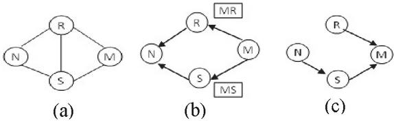
Figure 5 The algorithm for generating approximation minimum spanning tree.
4.3 Cluster Coverage
In the reference [29], the random deployment, the rule deployment and the planned deployment were discussed. In the random deployment, the nodes in a monitored area meet uniform distribution. In the rule deployment, the nodes are placed according to a regular geometric topology, such as the grids. In the planned deployment, the node density of key section in a monitoring area is higher than that of the general areas. This paper only focuses on the random deployment and the planned deployment. In the planned deployment, for the entire monitored area, although the deployment of nodes does not conform to the random uniform distribution, the deployment of nodes is close to be random in the small range. So the following analysis results for the random deployment are also applicable to the planned deployment. It is impossible to ensure that the nodes to be deployed cover the entire area in a random deployment, so this paper attempts to address the following issues: In the monitored area C with the radius R, in the case of the random deployment, how many nodes with the sensing radius r are required to ensure that the covered area in the entire area can achieve the desired value. For the convenience of description, it makes the center coordinate of C be (0, 0) and defines as follows:
Definition 1 The neighbour area. For (x, y) C, the definition of its neighbour areas is as follows:
| (8) |
Definition 2: The area . For the area , there is . And for any point , , the following relation is required:
| (9) |
For , if one node at least is contained by its neighbour area, then the point (x, y) is covered. Since the deployment of nodes in C conforms to the uniformly distribution, the probability that the nodes may be placed in the neighbour area of the point (x, y) is . It is assumed that m nodes are deployed in C, the probability of the point (x, y) being covered by these nodes is as following.
| (10) |
For , the size of its neighbour area is , so the probability that a single node may being placed in the neighbour area is . For , if there are m nodes with random deployment in C, based on the formula (9), the probability of this point being covered by these nodes is as following.
| (11) |
In the case where the node density is sufficient, the cluster constructed in each T phase can cover the entire monitored area A. Although the theoretical size of a cluster is , but in order to cover the monitored area A, there is an overlap between the neighbour clusters, that is, the actual range of the cluster is less than . Therefore, the number m of required nodes to achieve the covering value can be worked out approximately by the formula (11) according to the p designed by the specific application. In order to save energy, CH randomly select m nodes from its own cluster members as data collection nodes of the current round, and let the other members go into the sleep during the current round. The cluster head can dispatch its members by the intra-cluster broadcast TDMA.
5 Performance Analysis
5.1 Parameter Setting
ECAP protocol uses GlomoSim as the platform for simulation experiments, the experiment parameters are in Table 1. In the experiments, the network lifetime includes three different meanings: the death of the first node, the death of a half of the nodes and the death of the last node. In addition, in the simulation experiments, it is assumed that the perceived radius r of each node is 12 m. And when the node energy is less than the E (0.002 J), the node is considered dead.
Table 1 Simulation parameter
| Parameter | Value |
| Network size | (100100), (150 150), (200 200), (250 250), |
| (300 300), (350 350) | |
| Sink Position | (50,175), (50,200), (20,215), (50,230), (50,245), (50,260), |
| (50,275), (50,300), (50,400) | |
| Node number | 100,150,200,250,300,350,400450,500,1000 |
| Threshold distance(d0) | 75 m |
| Cluster radius(rc) | 30 m |
| Coverage radius(rs) | 12 m |
| Eelec | 50 nJ/bit |
| e_fs | 13 pJ/bit/m |
| e_mp | 0.0013 pJ/bit/m |
| E_fusion | 5 nJ/bit |
| Data Packet size | 500 bytes |
| Broad packet size | 25 bytes |
| Packet header size | 25 bytes |
| round | 5 TDMA frames |
| Initial energy | 2 J |
In order to compare the four protocols of DIRECT, LEACH, PEGASIS and ECAP, this paper simulated respectively the influence of the changes of the size of the monitored area, the changes of BS’s location and the number change of nodes on their performance. The results and analysis are shown in Section 4.3. In the simulation experiments, ECAP protocol is further divided into and ECAP-2 adopting the cluster coverage algorithm and general ECAP-1.
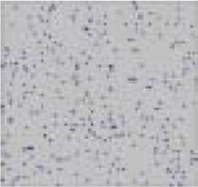
Figure 6 The distribution of nodes.
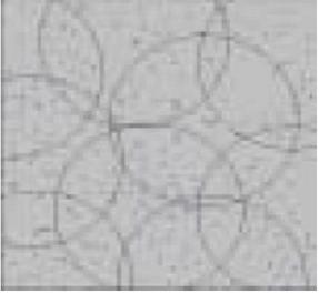
Figure 7 The distribution of cluster heads at 420th round.
5.2 Number and Distribution of Cluster Head
In order to verify that ECAP protocol can construct the clusters with the good distribution, the experiments randomly take 200 samples of the number of cluster heads and the distribution of cluster heads from two scenarios with 100 m 100 m and 200 m 200 m. The minimum number of cluster heads required to cover the monitored area A is N, according to the formula (3), then there is . The experiments show that after running ECAP protocol in each round, the number of the samples that the number of generated cluster heads is no more than accounts for 98% of all the samples, where, in the worst case, the number of generated cluster heads is . The experiment results illustrate that the number of generated cluster heads in each round is connected with r and the size of A. And the constructed clusters in A have good distribution. Figure 6 is the distribution graph of the nodes in a scenario with 100m 100m and the node number of 300. Figure 7 shows the cluster head distribution in the network at 420th round. It can be seen from these two figures that the distance between any two cluster heads is greater than r, and the clusters constructed by these cluster heads have fully covered all nodes in the network.
5.3 Experimental Results and Analysis
When the base station location is at (50, 245), the size of monitored area A is 100 m 100 m and the number of nodes is 100, Figure 8 showed the relationship of the number of dead nodes with the working time of network (the number of rounds). It can be seen that the curve of ECAP protocol in Figure 8 is almost a straight line parallel to the X axis. Because ECAP protocol can distribute uniformly the energy overhead to each node in the sensor network, the time that the first node and the last node die is very close, usually within 40 rounds. As can be seen from Figure 8, compared with LEACH protocol and PEGASIS protocol, ECAP protocol extends the network lifetime by 310% and 55% (the death the first node) respectively. Moreover, since the node density in the A is small, ECAP-2 protocol with the cluster covering algorithm cannot significantly extend the network lifetime, its performance slightly better than ECAP-1protoco.

Figure 8 The time of node death in a network with the size 100 m 100 m.
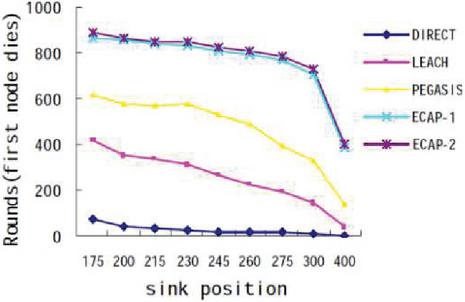
Figure 9(a) The relationship of the distance between network and BS with network lifetime (FDN).
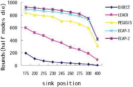
Figure 9(b) The relationship of the distance between network and BS with network lifetime (HDN).
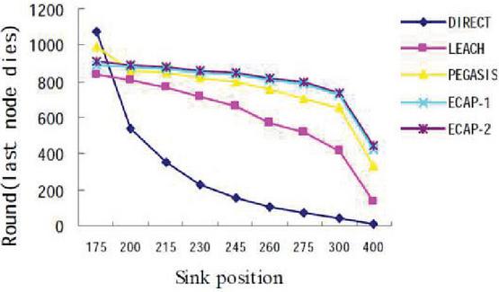
Figure 9(c) The relationship of the distance between network and BS with network lifetime (LDN).

Figure 10(a) The relationship of the size of network with network lifetime (FDN).
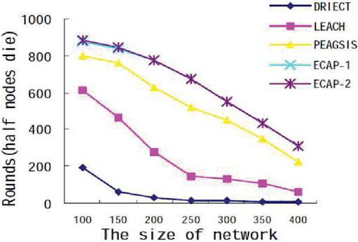
Figure 10(b) The relationship of the size of network with network lifetime (HDN).
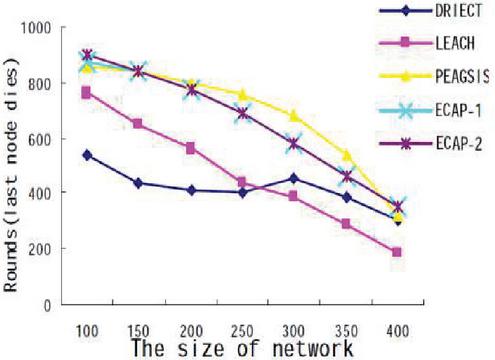
Figure 10(c) The relationship of the size of network with network lifetime (LDN).
From Figure 9, they respectively describe the relationship between the base station location and the three kinds of network lifetime that the death of the first node (FDN), the death of a half of nodes (HDN) and the death of the last node (LDN). Figure 8(a) shows that when the network lifetime is defined as FND, the reducing speed of network lifetime of ECAP protocol is slowest as the distance between the A and the base station increases. The experiments show that when the coordinate of BS is changed from (50,175) to (50,300), the network lifetime is reduced from 892 rounds to 732 rounds. Although the reduction is less than 18%, it is much better than that of PEGASIS and LEACH protocols. At the same time, it can be seen that the curve change of ECAP protocol in the three protocols is smallest, which means that in the sensor network running ECAP protocol, the difference of time among three kinds of network lifetime is very small.
The experiments consider the effect of the size of the A on the performance of three protocols. As can be seen from Figure 10, ECAP protocol can still maintain good performance as the size of A grows. The reasons are that there is a rational distribution of clusters in ECAP protocol, and the data is sent to BS by the multi-hop method to reduce the energy overhead of CHs so as to ensure that the performance of ECAP protocol is superior to LEACH protocol and PEGASIS protocol under the same conditions.
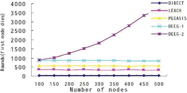
Figure 11 Network lifetime as the number of nodes increases (FDN).
Figure 11 shows the relationship of the number of nodes with the network lifetime. A noteworthy phenomenon is that that except ECAP-2, the above protocols cannot significantly extend the network lifetime as the number of nodes increases. The reason is that they did not consider the coverage problem of the nodes. Actually, when the node density is sufficient, a part of the nodes can cover the entire A. At this time, the other nodes are redundant and can sleep to reduce the overhead of energy to extend the network lifetime. Thus, except ECAP-2, all nodes are active in each round of the network running the other four protocols, so the network lifetime cannot be extended with the number of nodes increasing. In addition, since the CHs generated by ECAP protocol are only related to the size of the A and the distribution of nodes, the number of cluster members in ECAP-1 protocol increases as the number of nodes increases so as to lead to an increase in the energy overhead of the CHs, which further leads to advancing the time that the first node is to die. The figure still shows that when the number of nodes is 100, the time that the first node is to die is at the 890th round. And when the number of nodes is increased to 500, the time that the first node is to die is advanced to the 831st round. Since ECAP-2 protocol uses the cluster coverage method, when the number of member in a cluster goes beyond the practical application requirement, the cluster head in this cluster informs the redundant members to go in sleep. The experiments show that the network lifetime running ECAP-2 protocol increases linearly with the increase of the number of nodes.
For the protocols using rounds as a unit, the number of times that all active nodes collect the data in one round is consistent (this value is set to five in this experiments.), so the total number of times that all nodes in the network collect the environmental data can measure the performance of the corresponding protocol. According to the distance changes between the base station and the monitored area A, The sum of times that all nodes in the four protocols collect respectively the environmental data before the network failure (at the time of the first node to die) are computed and shown in Figure 10. It can be seen that the number of times for collecting the data in ECAP-1 protocol is much larger than that of the other three protocols(DIRECT protocol, LEACH protocol and PEGASIS protocol). And in the four protocols, as the distance between the base station and the monitored area A increases, the decreasing speed of the number of times for collecting the data in ECAP-1 protocol is slowest. This reason is that in ECAP protocol, the constructed cluster has good distribution in the network, and the data collected by each cluster is sent to the base station by the multi-hop method between the cluster heads, which can reduces the energy overhead of CHs and distribute uniformly the energy overhead to all the nodes. The simulation experiments show that the death time of the first node in ECAP protocol is usually within the last 40 rounds (the last node is dead). So the number of times for collecting the data in ECAP protocol is much larger than that of the other protocols, and the monitoring quality of ECAP protocol is higher than the other three protocols.
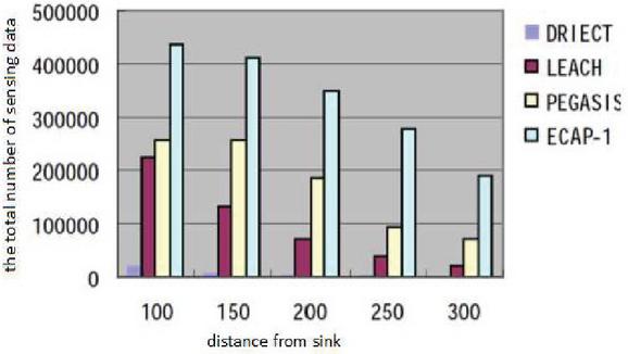
Figure 12 The total number of sensed data from all the nodes (FDN).
It can be seen from the experiment results that, except Figure 12, ECAP-1 and ECAP-2 protocols have similar performance in all graphs. The reason is that the node density is small and the redundant nodes are few so th at ECAP-2 protocol using the cluster coverage algorithm cannot also obviously extend the network lifetime. And when the redundant nodes increases, it can be seen from Figure 11 that the network lifetime running ECAP-2 protocol is much better than the other four protocols (DIRECT protocol, LEACH protocol, PEGASIS protocol and ECAP-1). However, in the T phase of ECAP protocol, all the nodes must be active and participate in the work constructing the clusters so as to consume energy, so when the number of redundant nodes reach a certain limit, the network lifetime will be no longer extended as the number of the nodes increases. In addition, the experiments show that the energy consumed by ECAP protocol in the T and T phases accounts for 0.4% to 0.7% of the total energy, which is comparable to PEGASIS protocol and greater than LEACH protocol (the energy consumed by LEACH protocol in the T phase accounts for 0.05% to 0.07% of the total energy).
6 Conclusions and Future Work
This paper presents a distributed protocol for efficient data collection and aggregation of wireless sensor networks. In the proposed protocol, the node competes for the cluster heads based on the residual energy and the signal strength of the neighbouring node. Once the cluster head is selected, the ordinary node will select a nearest cluster head to join so as to construct a cluster. In order to further save the energy, the CHs far from BS send the collected data to BS by the multi-hop method. In addition, ECAP protocol can extend the network lifetime by a simple cluster-covered algorithm when the node density is increased. The experiments show that ECAP protocol can extend the network lifetime, and get the death of all nodes to concentrate in the last 40 rounds, so that the monitoring results based on ECAP protocol are more accuracy.
WSN are often deployed in the areas where people are difficult to maintain. Because of the harsh environmental factors, the sensor node generally has a high failure rate. So if the cluster head are failure, in the sensor network running the cluster algorithm with single cluster head, then the collected data from all members will be lost. For achieving the better fault tolerance, the future work will improve the reliability in data collection and transmission on the basis of the proposed protocol.
Acknowledgements
This work sponsored by the National Natural Science Foundation of China (No.11261037) and the Nation Science Foundation of Shanghai (No.19ZR1420000).
References
[1] Mohammad Alibakhshikenari1, Bal S. Virdee , P. Shukla etc. Meta-Surface Wall Suppression of Mutual Coupling between Microstrip Patch Antenna Arrays for THz-Band Applications. Progress In Electromagnetics Research Letters, Vol. 75, 105–111, 2018.
[2] Kasilingam Rajeswari, Subbu Neduncheliyan. Genetic algorithm based fault tolerant clustering in wireless sensornetwork. IET Communications, Volume 11, Issue 12, August 2017, p. 1927–1932.
[3] H. Lee and A. Keshavarzian. Towards energy-optimal and reliable data collection via collision-free scheduling in wireless sensor networks. In INFOCOM, 2008.
[4] A Mohammad, BS Virdee, A Abdul, L Ernesto. A novel monofilar-archimedean metamaterial inspired leaky-wave antenna for scanning application for passive radar systems. Microwave and Optical Technology Letters, 15 June 2018.
[5] Y. Wu, Z. Mao, S. Fahmy, N. Shroff, Constructing maximum-lifetime data–gathering forests in sensor networks, IEEE/ACM Trans. Netw. 18(5) (2010) 1571–1584.
[6] Seong Yun Cho. Implementation Technology for Localising a Group of Mobile Nodes in a Mobile Wireless Sensor Network, Vol 67, November 2014, pp. 1089–1108
[7] W.-W. Ji, Z. Liu. Locating ineffective sensor nodes in wireless sensor networks. IET Communications, Volume 2, Issue 3, 2008, pp. 432–439.
[8] Pottie GJ, Kaiser WJ. Wireless integrated network sensors. Communications of the ACM, 2000, 43(5):51–58.
[9] Mallika Mhatre, Anoop Kumar, C. K. Jha. Energy-efficient WSN using membership handshaking clustering technique for isolated nodes. Pervasive Computing: A Networking Perspective and Future Directions. pp. 145–152, 30 January 2019.
[10] Yanjun Yao, Qing Cao, and Athanasios V. Vasilakos. EDAL: An energy-efficient, delay-aware, and lifetime-balancing data collection protocol for heterogeneous wireless sensor networks, IEEE/ACM Transactions on Networking Vol. 23(3), 2015, pp. 810–823.
[11] M. shobnan, R. Sabitha, S.Karthik. Cluster-based systematic data aggregation model (CSDAM) for real-time data processing in large-scale WSN. Wireless Personal Communications. 13 January 2020, 7(5): 16–27.
[12] Gaurav Bathla, Rajneesh Randhawa. Enhancing WSN lifetime using TLH: A routing scheme. Networking Communication and Data Knowledge Engineering. 14 November 2017, pp. 25–35.
[13] D. Luo, X. Zhu, X. Wu, G. Chen. Maximizing lifetime for the shortest path aggregation tree in wireless sensor networks, in: INFOCOM, 2011 Proceedings IEEE, April, 2011, pp. 1566–1574.
[14] Y. Wu, Z. Mao, S. Fahmy, N. Shroff. Constructing maximum-lifetime data–gathering forests in sensor networks, IEEE/ACM Trans. Netw. 18(5) (2010) 1571–1584.
[15] S. S. Jaspal, Umang, Brijesh Kumar. Energy saving using memorization: A novel energy efficient and fault tolerant cluster tree algorithm for WSN. Intelligent Decision Support Systems for Sustainable Computing. volume 70, pp. 179–206 (2017).
[16] M. C. Rajalakshmi, A. P. Gnana Prakash. MLO: Multi-level Optimization to Enhance the Network Lifetime in Large Scale WSN. Emerging Research in Computing, Information, Communication and Applications. pp. 265–271, 18 July 2015.
[17] Hongzhu Yue, Qijie Jiang, Chuanbin Yin, Jonny Wilson. Research on data aggregation and transmission planning with Internet of Things technology in WSN multi-channel aware network. The Journal of Supercomputing. Volume 76, pages 3298–3307 (2020).
[18] Jing (Selena) He, Shouling Ji, Yi Pan, and Yingshu Li, Constructing Load-Balanced Data Aggregation Trees in Probabilistic Wireless Sensor Networks, Transactions On Parallel And Distributed Systems, vol. 25(7), 2014.
[19] Shuai Gao, Hongke Zhang, and Sajal K. Das, Efficient Data Collection in Wireless Sensor Networks with Path-Constrained Mobile Sinks, IEEE Transactions on Mobile Computing, vol. 10(5), 2011.
[20] S. Ji, R. Beyah, Z. Cai, Snapshot/continuous data collection capacity for largescale probabilistic wireless sensor networks, in: IEEE International Conference on Computer Communications, INFOCOM, 2012, pp. 1035–1043.
[21] B. Dezfouli, M. Radi, K. Whitehouse, S.A. Razak, T. Hwee-Pink, Dicsa: distributed and concurrent link scheduling algorithm for data gathering in wireless sensor networks, Ad Hoc Netw. 25 (Part A) (2015) 254–271. [Online]. Available: http://www.sciencedirect.com/science/article/pii/S1570870514002005
[22] Heinzelman WR, Kulik J, Balakrishnan H. Adaptive protocols for information dissemination in wireless sensor networks. In: Proc. of the 5th Ann. Int’l Conf. on Mobile Computing and Networking. 2001. 174–185.
[23] Lindsey S, Raghavendra CS. Pegasis: Power-Efficient gathering in sensor information systems. In: Proc. of the IEEE Aerospace Conf. 2002. 1–6.
[24] Tan HO. Power efficient data gathering and aggregation in wireless sensor networks. SIGMOD Record, 2003.
[25] Bandyopadhyay S, Coyle E. An energy-efficient hierarchical clustering algorithm for wireless sensor networks. In: Proc. of the IEEE INFOCOM. 2003.
[26] Younis O, Fahmy S. Distributed clustering in Ad-hoc sensor networks: A hybrid, energy-efficient approach. In: Proc. of the IEEE INFOCOM. 2004.
[27] Heinzelman WR. An application-specific protocol architecture for wireless microsensor networks. IEEE Trans. on Wireless Communications, 2002, 1(4):660-670.
[28] Slijepcevic S, Potkonjak M. Power efficient organization of wireless sensor networks. In: IEEE Int’1 Conf. on Communications (ICC). 2001.
[29] Tilak S, Abu-Ghazaleh N, Heinzelman W. Infrastructure tradeoffs for sensor networks. In: Proc. of 1st Int’l Workshop on Wireless Sensor Networks and Applications (WSNA 2002). 2002. 49–57.
Biographies

Peng Xiong, received the B.Sc. degree and M.Sc. degree in Electrical Engineering from Nanchang University China in 1998 and 2004, respectively, and Ph.D. degree in Computer science and technology from East China Normal University China in 2009. From 2010 on, he is a faculty member in the school of electronic information, Shanghai Dianji University China. He is a member of China Computer Federation (CCF), and his research is currently focused on network secure, wireless networks, cloud computing and big data etc.

Qinggang Su, received the B.Sc. degree in Computer Science from Anhui University of Technology in 2002, and got the M.Sc. degree in Communication Engineering in Shanghai Jiao Tong University, and is studying for Ph.D. degree at East China Normal University. He became a faculty member in the school of electronic information, Shanghai Dianji University China from 2002, and he is rhe vice dean of Chinesisch-Deutsche Kolleg für Intelligente Produktion of Shanghai Dianji University now. He is a member of China Computer Federation (CCF), and his research is currently focused on wireless networks, 5G application and smart manufacturing.
Journal of Web Engineering, Vol. 20_3, 615–640.
doi: 10.13052/jwe1540-9589.2033
© 2021 River Publishers