Towards the Importance of the Type of Deep Neural Network and Employment of Pre-trained Word Vectors for Toxicity Detection: An Experimental Study

Abdullah Talha Kabakus

Department of Computer Engineering, Faculty of Engineering, Duzce University, Turkey

E-mail: talhakabakus@duzce.edu.tr

Received 18 February 2021; Accepted 30 July 2021; Publication 27 October 2021

Abstract

As a natural consequence of offering many advantages to their users, social media platforms have become a part of their daily lives. Recent studies emphasize the necessity of an automated way of detecting offensive posts in social media since these ‘toxic’ posts have become pervasive. To this end, a novel toxic post detection approach based on Deep Neural Networks was proposed within this study. Given that several word embedding methods exist, we shed light on which word embedding method produces better results when employed with the five most common types of deep neural networks, namely, Convolutional Neural Network (CNN), Long Short-Term Memory (LSTM), GRU (Gated Recurrent Unit), Bidirectional Long Short-Term Memory (BiLSTM), and a combination of CNN and BiLSTM. To this end, the word vectors for the given comments were obtained through four different methods, namely, ($i$) $Word2vec$, ($ii$) $fastText$, ($iii$) $GloVe$, and ($iv$) the $Embedding$ layer of deep neural networks. Eventually, a total of twenty benchmark models were proposed and both trained and evaluated on a gold standard dataset which consists of $16K$ tweets. According to the experimental result, the best $F1-score$, $84.844\%$, was obtained on the proposed CNN model without employing pre-trained word vectors which outperformed the state-of-the-art works and implies the effective embedding ability of CNNs. Other key findings obtained through the conducted experiments are that the models, that constructed word embeddings through the $Embedding$ layers, obtained higher $F1-score$s and converged much faster than the models that utilized pre-trained word vectors.

Keywords: Word embedding, word vector, deep neural network, convolutional neural network, recurrent neural network, toxic comment detection.

1 Introduction

Social media platforms have become the essential reason for using the web in the last decade as a recent report by the cooperation of We Are Social and Hootsuite highlights that almost $85\%$ of the web users ($3.8$ billion of $4.5$ billion) use social media platforms and almost $60\%$ of the world’s population uses the web [1]. Social media platforms let users share their opinions on anything they want. Alongside sharing their own opinions, people tend to use these platforms to seek others’ opinions about anything they are interested in. During this bi-directional opinion sharing on these platforms, debates happen due to the ability to add comments. Cyberbullying has been defined by many national crime prevention councils as most studies reported that the prevalence rates of cyberbullying range from $10\%$ to $40\%$ of internet users [2]. The effects of cyberbullying vary from temporary anxiety to suicide [3]. When one of these sides uses ‘toxic comments’ as a result of using offensive language, unfortunately, virtual fights do happen which can lead people both to stop expressing themselves and to stop seeking others’ opinions out of fear of abuse through social media platforms [4] which eventually means less number of visitors and less money when the subscription models and ads are considered [5]. Also, legal reasons might require these platforms to propose countermeasures against the toxic comments such as actively monitoring all the available content on the platform and deleting when such comments are detected within $24$ hours [5]. Therefore, a mechanism for the detection of these toxic comments is a key necessity for social media platforms to let people use these platforms without any concerns. This detection mechanism needs to be ‘automated’ to not be time-consuming and labor-intensive when the fact that an enormous volume of content posted daily on the social media platforms was considered. Toxic comment detection is a challenging task. First of all, what makes a comment ‘toxic’ is quite subjective. Not all comments that contain swear words convey negative meanings as expected. One example of this case is that $78\%$ of the swearing posts in the Formspring,¹ a question-and-answer-based social network, are actually non-toxic comments [6]. Similarly, it is reported that $82\%$ of the toxic tweets in a Twitter toxic comment (tweet) dataset do not use any swear words [6]. Therefore, the presence of swear words is neither necessary nor sufficient to regard a comment as ‘toxic’ [6]. A toxic comment is generally classified into five classes as follows [5]: ($i$) obscene language, ($ii$) insult, ($iii$) threat, ($iv$) identity hate, and ($v$) severe toxic.

The first step of detecting toxic comments is understanding the content of these comments. Word embeddings are the vectorial representations of words that each vector consists of real numbers. This mapping lets creating more compact and expressive word presentations [7] that can be utilized with many machine learning algorithms. Word embedding has been widely used in Natural Language Processing (NLP) applications such as machine translation [8], conversational dialog systems, and sentiment classification [9]. Words can be represented as vectors or bag-of-words. The biggest advantage of utilizing vector representations, that are constructed through word embeddings, instead of the bag-of-words representation, is that vector representations are capable of capturing the semantic meaning of the text [10]. Various types of deep neural networks have demonstrated the state-of-the-art in many domains. In addition to various deep neural networks, there exist various widely used state-of-the-art word embedding methods in the literature. Therefore, the main motivation of this study is to shed light on which type of deep neural network and which word embedding method provide the best performance for toxic detection. To this end, in this study, a total of twenty models based on the five most commonly used types of deep neural networks, namely, Convolutional Neural Network (CNN), Long Short-Term Memory (LSTM), GRU (Gated Recurrent Unit), Bidirectional LSTM (BiLSTM), and a combination of $CNN$ and $BiLSTM$, were proposed with utilizing three state-of-the-art word embedding methods, namely, $Word2vec$ [11, 12], $fastText$ [13], and GloVe (Global Vectors for Word Representation) [14] for toxic detection on a gold standard dataset. The main contributions of this study are given as follows:

• A total of twenty models based on the five types of widely-used deep neural networks, namely, $CNN$, $LSTM$, $GRU$, $BiLSTM$, and a combination of $CNN$ and $BiLSTM$, were experimented in order to reveal the performance differences of these deep neural networks for the toxic detection task.

• The effects of various word embedding methods on the proposed deep neural network models were investigated in order to shed light on which embedding method provides a better result for the toxic comment detection task when it is deployed with a deep neural network.

• Instead of utilizing handcrafted features, which are not robust against the variations of writing style, the features of the proposed models were automatically extracted thanks to the proposed deep neural network models.

• Instead of training the deep neural networks for a fixed number of epochs, the training process was dynamically managed thanks to an employed callback. To the best of our knowledge, this is the first study in the literature on toxic comment detection that employed this technique.

• The learning rate of each proposed deep neural network was adapted to the performance of the network thanks to an employed callback. To the best of our knowledge, this is the first study in the literature on toxic comment detection that employed this technique.

2 Related Work

Davidson et al. [15] employed a variety of traditional machine learning algorithms, namely, Logistic Regression, Naïve Bayes, Decision Tree, Random Forest, and Linear SVM, for hate speech detection. To this end, they utilized the Twitter API to construct their own dataset to evaluate the employed models. According to the experimental result, the best performing model, which was based on Logistic Regression with L2 regularization, achieved an overall $precision$ of $0.91$, a $recall$ of $0.90$, and an $F1-score$ of $0.90$ on the constructed dataset. They also reported that both Logistic Regression and Linear SVM significantly better performance than the other models.

Zhang et al. [16] proposed an approach for toxic detection that was based on a deep neural network that was a combination of Convolutional and GRU networks. According to the conducted experiments, the best $F1-score$, $0.94$, of the proposed model was obtained on the dataset constructed by Davidson et al. [15]. Another finding of this study was that the proposed model outperformed the other SVM and CNN models. Similar to our model, they implemented their model by using Keras. But unlike our implementation, they employed Theano as the backend of Keras instead of TensorFlow.

Badjatiya et al. [17] investigated hate speech detection on Twitter. To this end, they employed three methods, namely, ($i$) CNN, ($ii$) LSTM, and ($iii$) fastText. When it comes to word embedding, they utilized two methods to initialize the word embeddings, namely, ($i$) random embeddings, and ($ii$) GloVe embeddings. According to the experimental result, the proposed LSTM model with Gradient Boosted Decision Trees on the randomly initialized embeddings achieved the best performance on a Twitter dataset [18] with providing a $precision$, $recall$, and $F1-score$ of $0.73$. It is worth mentioning that, as the authors mentioned in the paper, the random embedding method surprisingly yielded a better performance for their model. The methodological issue in this study is that they extracted the features by utilizing the complete labeled dataset which leads to an artificial increase in the performance of the model while underestimating the generalization error as a result of overfitting [19]. This issue was discussed in detail by Arango et al. [19] and they reported that replication of this model obtained a macro averaged F1-score of $73.1\%$ when this methodological issue was taken into account. They trained the models for a fixed number ($10$) of epochs. Unlike this training preference, the number of epochs the model was trained for was dynamically set for the proposed model which means that the training was stopped when the model’s performance has started decreasing. Another difference in terms of model training is that the learning rate of the proposed model was dynamically adapted through the performance of the model in the last epochs.

Zampieri et al. [20] proposed an approach to detect both the toxic language and the type of toxic in social media. To this end, they experimented on three methods, namely, ($i$) SVM, ($ii$) BiLSTM, and ($iii$) CNN. In order to evaluate the proposed models based on the aforementioned methods, they complied a new Twitter dataset, namely, OLID (Offensive Language Identification Dataset) which consisted of a total of $14,100$ tweets. According to the experimental result, the best $Macro-F1$ $score$, $0.80$, was obtained by the proposed CNN model for the toxic language detection task.

Park and Fung [21] proposed three methods based on CNN to classify sexist and racist abusive language, namely, ($i$) CharCNN which is a character-level CNN, ($ii$) WordCNN which segments the input sentences into words and converted into $300$-dimensional embeddings, and ($iii$) HybridCNN which is a combination of CharCNN, and WordCNN that utilizes both character and word inputs. They utilized the Twitter datasets provided by Waseem and Hovy [18] and concatenated them into a new one. Then they divided this concatenated dataset into three datasets as follows: ($i$) “One-step” dataset that aims multi-class segmentation for the labels “$none$”, “$racism$”, and “$sexism$”, ($ii$) “Two-step-1” dataset that merges the “$sexism$”, and “$racism$” labels into one abusive label and aims abusive language detection, and ($iii$) “Two-step-2” dataset that consists of the labels “$none$”, and “$abusive$” in order to experiment a classifier to distinguish “$sexism$” and “$racism$”. According to the experimental result, the proposed HybridCNN achieved an $F1-score$ of $0.827$ on the “One-step” dataset and the Logistic Regression achieved an $F1-score$ of $0.824$ on the “Two-step” dataset.

Twitter is not the only social media platform that has been investigated for the toxic detection task. Van Hee et al. [22] utilized the ASKfm, an online question-and-answer platform, to construct a dataset. The constructed dataset comprised $113,698$ manually annotated posts written in English. They proposed a model based on Linear SVM and evaluated its performance on their own dataset. The proposed model was tuned thanks to the Grid Search, a widely-used tuning method to reveal the optimum values of hyper-parameters. According to the experimental result, the proposed model achieved an $F1-score$ of $0.6426$. In addition to the ASKfm, Wikipedia was also utilized for toxic detection task in the literature. Chakrabarty [23] proposed an approach based on a $6$-headed machine learning TF-IDF (Term Frequency-Inverse Document Frequency) model. This proposed model was evaluated on a labeled Wikipedia comment dataset and the model achieved a $Macro-F1score$ of $0.9817$. Similar to the ASKfm, Formspring is another online question-answer platform that was utilized for the toxic detection task. Reynolds et al. [24] constructed a dataset by crowd-sourcing the Formspring platform which consisted of $3,915$ posts. In order to label these posts, the authors utilized the Amazon Mechanical Turk service, an online service to set labels for the given datasets. They employed a C4.5 decision tree and an instance-based learner for toxic detection on the constructed dataset. According to the experimental result, both learners achieved an $accuracy$ of $78.5\%$ for the true positives. Agrawal and Awekar [6] proposed deep neural networks, which were similar to the models proposed by Badjatiya et al. [17], for detecting toxic comments on Twitter, Formspring, and Wikipedia. They experimented with four types of deep neural networks, namely, ($i$) CNN, ($ii$) LSTM, ($iii$) BiLSTM, and ($iv$) BiLSTM with an attention mechanism. They evaluated the proposed models on the same dataset of Badjatiya et al. [17] but they oversampled the data from the “$hate$” class after observing that only a few posts were marked as “$hate$” for their training set. The methodological issue here is that they oversampled the dataset before the train-test split which is a reason for the ‘overfitting’ problem [19]. This issue was discussed in detail by Arango et al. [19] and they reported that replication of this model obtained a macro averaged F1-score of $79.6\%$ when this methodological issue was taken into account. Similar to Badjatiya et al. [17], the models within this study were trained for $10$ epochs.

3 Material and Method

In this section, first, the employed word embedding models are briefly described. Second, the proposed deep neural network models for toxic detection are described. Finally, the gold standard dataset that was used by the proposed models is described.

3.1 Word Embedding Methods

In the following subsections, the three employed word embedding methods, namely, ($i$) $Word2Vec$, ($ii$) $fastText$, and ($iii$) $GloVe$, are briefly described. The word embedding models based on these methods were implemented using a widely used Python library, namely, gensim [25].

3.1.1 Word2Vec

$Word2vec$ is a state-of-the-art technique to efficiently create word embeddings from a given text, which is generally a large corpus of text. $Word2vec$ was proposed in 2013 by a team whose members work at Google.

3.1.2 GloVe

$GloVe$ is a global log-bilinear regression model for unsupervised learning of word representations that aims to represent words as numerical sequences that are trained on aggregated global word-word co-occurrence statistics from a corpus. $GloVe$ was proposed in 2014 and was developed as an open-source project at Stanford University.

3.1.3 fastText

$fastText$ is another widely used word embedding method that is based on $Word2vec$ and developed by Facebook AI Research (FAIR) lab. The initial version of $fastText$ was released in 2015. The advantages of $fastText$ are listed as follows: ($i$) It is robust for rare words, ($ii$) it is able to group inflected words, and ($iii$) it is fast to compute [26].

An overview of the employed word embedding methods within this study is listed in Table 1. In order to compare the performance of the word embedding methods, their pre-trained models, which were trained on the same corpus, namely, Common Crawl, were employed. Alongside these methods, as an additional embedding method, the pre-trained word vectors were not given to the proposed deep neural networks in order to reveal the efficiency of deep neural networks to create word vectors from the given textual data.

Table 1 An overview of the employed word embedding methods

Model	Embedding Method	Vector Size	Vocabulary Size	Corpus
$E_1$	$Word2vec$	$300$	$2.8M$	Common Crawl
$E_2$	$fastText$	$300$	$1M$	Common Crawl
$E_3$	$GloVe$	$300$	$1.2M$	Common Crawl

3.2 Proposed Deep Neural Network Models

A total of twenty models, which were based on the five of the most popular deep neural networks, namely, ($i$) $CNN$, ($ii$) $LSTM$, ($iii$) $GRU$, ($iv$) $BiLSTM$ [27], and ($v$) a combination of $CNN$ and $BiLSTM$, were proposed to reveal the efficiency of employing the pre-trained word vectors instead of the word embedding ability of deep neural networks. In the following subsections, the proposed deep neural network models are described. The proposed models were implemented using Keras [28], which is a Python library and acts as a wrapper for various backends. TensorFlow [29], an open-source machine learning library developed by Google, was employed as the backend of Keras since it is the recommended one [30] by the developer of Keras, who also works as a software engineer at Google. The proposed models were experimentally designed as there are no clear rules that can be applied to any kind of deep neural networks except the best practices, which were strictly followed. An overview of the proposed model is presented in Figure 1. The pseudocode of the proposed model is listed in Table 2.

Figure 1 An overview of the proposed model.

Table 2 The pseudocode of the proposed model

Preprocess data

Load all tokens into a list and assign to $\mathit{t}$

Calculate maximum sequence length of $\mathit{t}$ and assign to $\mathit{m}\mathit{a}\mathit{x}\mathbf{\_}\mathit{l}\mathit{e}\mathit{n}$

Construct word embeddings according to $\mathit{m}\mathit{a}\mathit{x}\mathbf{\_}\mathit{l}\mathit{e}\mathit{n}$

Construct deep neural network model

Define patience and monitored criterion as $\mathit{p}$, and $\mathit{c}\mathit{r}\mathit{i}\mathit{t}$

Train deep neural network

Set learning rate to 0.001 and assign to $\mathit{l}\mathit{r}$

Factor $\mathit{l}\mathit{r}$ by 0.1 when $\mathit{c}\mathit{r}\mathit{i}\mathit{t}$ is not improved

Stop training when $\mathit{c}\mathit{r}\mathit{i}\mathit{t}$ is not improved for $\mathit{p}$

Evaluate deep neural network

Figure 2 A plot of the distribution of the lengths of the tweets ($doc\mathrm{\_}len$).

3.2.1 Proposed CNN model

The proposed $CNN$ model consisted of $6$ layers. The model starts with an $Embedding$ layer to utilize or construct the word embeddings for the given comments. The input length of the $Embedding$ layer (denoted with $max\mathrm{\_}len$), $22$, was determined by the sum of the mean of the length of each tweet (denoted with $doc\mathrm{\_}len$) with the standard deviation (denoted with $std$) of the $doc\mathrm{\_}len$ as the corresponding equation is given in Equation (1). A plot of the distribution of the lengths of tweets ($doc\mathrm{\_}len$) is presented in Figure 2. It is worth mentioning that each $Embedding$ layer in the proposed benchmark models was configured similarly.

$max\mathrm{\_}len=mean(doc\mathrm{\_}len)+std(doc\mathrm{\_}len)$

(1)

After the $Embedding$ layer, a convolutional layer (denoted with $Conv$) was employed to perform convolution operations on the input. After that, a $MaxPooling$ layer, which is responsible for reducing the dimensionality of the input by applying the maximum function on it, was employed. After the $Conv$ layer, a $GlobalMaxPooling$ layer was employed which sets the pool size to the input size to apply the maximum function to the entire input. Following this, a $Dropout$ layer, which is a widely used regularization technique that randomly drops neurons from the neural network to prevent the ‘overfitting’ problem [31], one of the biggest challenges of deep neural networks as a result of increased depth and complexity of deep neural networks [32, 33], was employed. Finally, a $Dense$ layer, which is a fully-connected neural network component that is responsible for classification, was employed. This $Dense$ layer was configured with $3$ outputs units since the aim of the model is a trinary classification. The $RectifiedLinearUnit(ReLU)$ [34] was employed as the activation function of the $Conv$ layer. The activation function of the $Dense$ layer was set to the $softmax$ since the aim of the model is to make a trinary prediction for each given tweet. $L2regularization$ was employed with this $CNN$ layer to the kernel weights matrix, bias vector, and the output of the layer to further prevent the overfitting problem in addition to the employed $Dropout$ layer [35]. The layers of the proposed $CNN$ model with their configuration parameters are listed in Table 3.

Table 3 The layers of the proposed $CNN$ model with their configuration parameters

Layer	Configuration Parameters
$Embedding$	– $inputdimension$: Total number of words in the vocabulary – $outputdimension$: $200$ – $inputlength$: Maximum length of the comments
$Dropout$	– $dropout\mathrm{\_}rate$: $0.8$
$Conv$	– $numberoffilters$: $64$ – $kernelsize$: $5$ – $activationfunction$: $ReLU$ – $padding$: $\mathrm{`}sam{e}^{\prime }$
$GlobalMaxPooling$	$-$
$Dropout$	– $dropout\mathrm{\_}rate$: $0.5$
$Dense$	– $numberofunits$: $3$ – $activationfunction$: $softmax$

3.2.2 Proposed LSTM Model

An $LSTM$ network is a special type of Recurrent Neural Network (RNN) that is capable of learning long-term dependencies thanks to having a long-term memory, and forget gates which lets the model overcome the general problem of gradient descent [36]. The proposed $LSTM$ model consisted of $5$ layers. Similar to the proposed $CNN$ model, the $LSTM$ model starts with an $Embedding$ layer to utilize the word embeddings for the given comments. After that, a $Dropout$ layer was employed to prevent the overfitting. Then, an $LSTM$ layer with $50$ output units was employed. After the $LSTM$ layer, another $Dropout$ layer was employed. Finally, a $Dense$ layer was employed for the classification. Similar to the proposed $CNN$ model, the final $Dense$ layer was configured with $3$ output units. The layers of the proposed $LSTM$ model with their configuration parameters are listed in Table 4.

Table 4 The layers of the proposed $LSTM$ model with their configuration parameters

Layer	Configuration Parameters
$Embedding$	– $inputdimension$: Total number of words in the vocabulary – $outputdimension$: $200$ – $inputlength$: Maximum length of the comments
$Dropout$	– $dropout\mathrm{\_}rate$: $0.25$
$LSTM$	– $numberofunits$: $50$
$Dropout$	– $dropout\mathrm{\_}rate$: $0.5$
$Dense$	– $numberofunits$: $3$ – $activationfunction$: $softmax$

3.2.3 Proposed GRU model

A $GRU$ is also another special type of $RNN$. The key difference between a $GRU$ and an $LSTM$ is that while an $LSTM$ has three gates, namely, ($i$) input, ($ii$) output, and ($iii$) forget gates, a $GRU$ has two gates, namely, ($i$) reset, and ($ii$) update gates. This architectural difference makes $GRU$ simpler, faster to train, and better on generalization on small data compared to $LSTM$ [16]. So, a new benchmark model was constructed solely based on this architectural difference from the constructed $LSTM$ model. Therefore, the $LSTM$ layer in the previous $LSTM$ model was replaced with a $GRU$ layer for this new benchmark model. The layers of the proposed $GRU$ model with their configuration parameters are listed in Table 5.

Table 5 The layers of the proposed $GRU$ model with their configuration parameters

Layer	Configuration Parameters
$Embedding$	– $inputdimension$: Total number of words in the vocabulary – $outputdimension$: $200$ – $inputlength$: Maximum length of the comments
$Dropout$	– $dropout\mathrm{\_}rate$: $0.25$
$GRU$	– $numberofunits$: $50$
$Dropout$	– $dropout\mathrm{\_}rate$: $0.5$
$Dense$	– $numberofunits$: $3$ – $activationfunction$: $softmax$

3.2.4 Proposed BiLSTM model

The proposed $BidirectionalLSTM(BiLSTM)$ model is very similar to the proposed $LSTM$ model as it consisted of $5$ layers. The only difference between these two models is that, unlike the proposed $LSTM$ model, the $LSTM$ layers in the $BiLSTM$ model are bidirectional which comes from the idea of presenting each training sequence forward and backward to two separate $RNN$s, both of which are connected to the same output layer [37]. In theory, this architectural modification lets capturing richer contextual information instead of using high-order factorization [38]. The layers of the proposed $BiLSTM$ model with their configuration parameters are listed in Table 6.

Table 6 The layers of the proposed $BiLSTM$ model with their configuration parameters

Layer	Configuration Parameters
$Embedding$	– $inputdimension$: Total number of words in the vocabulary – $outputdimension$: $200$ – $inputlength$: Maximum length of the comments
$Dropout$	– $dropout\mathrm{\_}rate$: $0.25$
$BiLSTM$	– $numberofunits$: $50$
$Dropout$	– $dropout\mathrm{\_}rate$: $0.5$
$Dense$	– $numberofunits$: $3$ – $activationfunction$: $softmax$

3.2.5 Proposed CNN$+$BiLSTM model

The proposed $CNN+BiLSTM$ model is a sequential model that consists of a $CNN$ and a $BiLSTM$ for encoding, and decoding, respectively. This model is a typical ‘encoder-decoder’ network. The layers of the proposed $CNN+BiLSTM$ model with their configuration parameters are listed in Table 7.

Table 7 The layers of the proposed $CNN+BiLSTM$ model with their configuration parameters

Layer	Configuration Parameters
$Embedding$	– $inputdimension$: Total number of words in the vocabulary – $outputdimension$: $200$ – $inputlength$: Maximum length of the comments
$Dropout$	– $dropout\mathrm{\_}rate$: $0.8$
$Conv$	– $numberoffilters$: $64$ – $kernelsize$: $5$ – $activationfunction$: $ReLU$ – $padding$: $\mathrm{`}sam{e}^{\prime }$
$BiLSTM$	– $numberofunits$: $50$
$Dropout$	– $dropout\mathrm{\_}rate$: $0.5$
$Dense$	– $numberofunits$: $3$ – $activationfunction$: $softmax$

3.3 Training Configuration

Since one of the aims of the proposed study is to shed light on the performance differences between the types of widely-used deep neural networks, all of the proposed deep neural network models were trained under the same configuration as follows: The Adaptive Moment Estimation (Adam) [39], which was proposed as an extension to the Stochastic Gradient Descent (SGD) [40], was employed as the optimization algorithm, which is responsible for updating the weights of the layers on the basis of the calculated loss. Another optimization algorithm, the Root Mean Square Propagation (RMSprop) has achieved a slightly worse performance than $Adam$. The Categorical Cross-Entropy function was employed as the loss function since our task is a multi-class classification problem. A loss function in a deep neural network is responsible for calculating the loss of the model for each iteration to let the model reduce the loss on the next iteration. The metric that was evaluated by the model was defined as $accuracy$. $20\%$ of the training set was used as the validation set. The $batchsize$, which is the number of samples utilized in one iteration, was set to $128$. The training was started with the $EarlyStopping$ callback, which is responsible for stopping the training when the model’s monitored metric has stopped improving for the pre-defined number of epochs (a.k.a. patience). As a result of this mechanism, the $EarlyStopping$ callback helps to prevent the overfitting problem [41–43]. The monitored metric and patience of the employed $EarlyStopping$ callback were defined as the $validationloss$ (the loss calculated for the validation set), and $5$, respectively. Another callback that was employed is the callback of reducing the learning rate of the model when the monitored metric has stopped improving. For this callback, similar to the $EarlyStopping$ callback, the $validationloss$ was monitored and the learning rate of the model was factored by $0.1$ when the $validationloss$ has not decreased for $2$ epochs. The lower bound of the learning rate was defined as $e^{-6}$. To the best of our knowledge, this is the first study in the toxic comment detection literature that employs these callbacks during the training of the deep neural network. The hyper-parameters of the employed $Adam$ algorithm were set after the model optimization (described in Section 3.6) and are listed in Table 8.

Table 8 The hyper-parameters of the employed $Adam$ algorithm

Hyper-parameter	Value
Learning rate	$0.001$
Beta 1	$0.9$
Beta 2	$0.999$
Epsilon	$e^{-8}$
Decay rate	$0.00001$

3.4 Data Preparation

The proposed models were both trained and evaluated on a gold standard toxic tweets dataset which was proposed by Waseem and Hovy [18] and consisted of $16K$ tweets. The dataset contains a label that defines the toxicity type alongside the Id (Identifier) of the tweet defined by Twitter for each tweet. Since the Twitter terms prohibit sharing the texts of tweets, the dataset contains the Ids of tweets instead of their texts. Thanks to the Tweepy [44], an open-source Python library for accessing the Twitter API, the texts of the tweets were retrieved through their Ids. This dataset was annotated by crowd-sourcing the tweets of more than $600$ Twitter users. The labels that were defined for the tweets in the dataset are “$racism$”, “$sexism$”, and “$neither$”. The proposed model within this study is a multi-class model that aims to classify the given samples into the given three labels, namely, ($i$) “$racism$”, ($ii$) “$sexism$”, and ($iii$) the “$neither$”. The preprocessing phase, whose effect on the performance of neural networks is proven [45], contains the following operations to prepare data to be ready to yield into the proposed deep neural network:

• The tweets were lowercased to regard any forms of a word in terms of the case (e.g., uppercase, lowercase, sentence case, etc.) the same.

• The meaningless parts of tweets in terms of toxicity detection, namely, weblinks, usernames, and mentions were cleared from the tweets.

• The punctuation marks and whitespace characters were cleared from the tweets.

• The prefix of declaring that a tweet is a retweet of another one, the “$RT$”, was cleared from the tweets.

• The stop words, which are the most common words in a language, were cleared from the tweets in order to focus on more important, meaningful words for the aim of the model. The stop words of English were obtained through a widely used Python library for NLP, namely, Natural Language Toolkit (NLTK) [46].

• The $173$ tweets, whose texts were completely removed (became empty Strings) after the aforementioned preprocessing operations, were dropped from the dataset.

The utilized $Twitter$ dataset ($D$) does not provide separated training and test sets. Therefore, the dataset was split into subsets as follows: $70\%$ of it ($11,834$ tweets), and $30\%$ of it ($5,073$ tweets) were utilized as the training set, and the test set, respectively. An overview of the utilized dataset is given in Table 9.

Table 9 An overview of the utilized $Twitter$ dataset

Dataset	Number of Samples Labeled with “Racism”	Number of Samples Labeled with “Sexism”	Number of Samples Labeled with “Neither”
$Twitter$ ($D$)	$1,976$	$3,430$	$11,501$

3.5 Model Optimization

There are no standard guidelines for the construction of deep neural networks. Deep neural networks contain many hyper-parameters, which are parameters whose optimal values are revealed empirically based on the performance evaluation of deep neural networks. This process is known as the ‘hyper-parameter optimization’ task and is very determinative on the performance of the trained network since hyper-parameters of deep neural networks significantly affect the training process. Therefore, a wide range of hyper-parameters was empirically experimented with in an automated manner to reveal their optimal values as they are listed in Table 10. To this end, an open-source Python library that was specifically designed for Keras and was recommended by the developer of Keras [30] for the hyper-parameter optimization task, namely, Hyperas [47], was employed. The proposed models, which are described in the previous subsections, were optimized according to the experimental result of hyper-parameter optimization.

Table 10 The experimented values of hyper-parameters during the hyper-parameter optimization of the proposed models

Hyper-parameter	Experimented Values/Algorithms
Activation function	$ReLU$, $tanh$, $sigmoid$, $softmax$
Optimization algorithm	$Adam$, $SGD$, $RMSprop$, $Adadelta$
Loss function	$BinaryCross-Entropy$, $CategoricalCross-Entropy$, $SparseCategoricalCross-Entropy$, $Poisson$, $KLDivergence$
Learning rate	$e^{-6},e^{-5},e^{-4},e^{-3},e^{-2}$
Momentum	$0.0$, $0.9$, $0.99$
Decay rate	$0.00001$, $0.0001$, $0.001$, $0.01$, $0.1$
Dropout rate	$0.25$, $0.5$, $0.6$, $0.7$, $0.8$
Kernel size	$3$, $5$, $7$
Number of filters	$8$, $16$, $32$, $64$, $128$, $256$
Number of units in $LSTM$ layers	$8$, $16$, $32$, $50$, $64$, $100$, $128$, $256$
Number of units in the $Dense$ layers (except for the last $Dense$ layer which was fixed to $3$)	$32$, $64$, $128$, $256$
Batch size	$64$, $128$, $256$
Number of $Conv$ layers	$1$, $2$, $3$
Number of $LSTM$/$GRU$/$BiLSTM$ layers	$1$, $2$, $3$

4 Experimental Result and Discussion

All the experiments that were conducted within this study were carried out on the Colaboratory (a.k.a. Google Colab) [48], which is a platform maintained by Google that provides free powerful GPUs alongside permanent (through the provided integration with the Google Drive service) and temporary storages. Google Colab comes with many useful Python data science libraries including but not limited to TensorFlow, Keras, scikit-learn, NumPy, and Pandas on a Linux server operating system. NLTK is one of these built-in libraries of Google Colab and it was utilized during the data preprocessing phase as is described in detail in the previous section. In addition to these advantages, it is possible to execute the Linux Command-Line Interface (CLI) commands on the provided machine which lets us download the necessary resources (e.g., the pre-trained word vectors for the utilized word embedding methods, the utilized dataset, the NLTK resources for English, etc.).

The motivations behind the conducted experiments were twofold: First, we shed light on the performance differences between the types of the most commonly used deep neural networks. Second, we shed light on the performance differences between various widely-used word embedding methods. To this end, a total of twenty benchmark models were constructed. The proposed models were both trained and evaluated on the utilized $Twitter$ dataset ($D$), which is described in the previous section. The confusion matrix is the de facto standard of measuring the efficiency of classifiers and defines the $accuracy$, $precision$, $recall$, and $F1-score$ evaluation metrics. Since the detection of the toxicity level is a classification problem, the confusion matrix was employed to measure the efficiency of the proposed model. While $\mathrm{`}Positiv{e}^{\prime }(P)$ corresponds to the target class of classifiers, $\mathrm{`}Negativ{e}^{\prime }(N)$ corresponds to the opposite class of the $P$. $Precision$ is the ratio of correctly classified $positives$ ($TP$) to all $positive$ predictions ($P$). $Recall$ (a.k.a. $TruePositiveRate$) is the ratio of correctly classified $positives$ ($TP$) to all (actual) $positive$ samples. $Accuracy$ is the ratio of correct predictions to all predictions. $Precision$ and $recall$ are often in tension since the improvement of $precision$ typically reduces the $recall$. $F1-score$ is the harmonic mean of $precision$ and $recall$ and takes both $FalsePositive(FP)$ and $FalseNegative(FN)$ scores into account. The higher the $F1-score$, the better is the result. $\mathrm{`}Tru{e}^{\prime }(T)$, and $\mathrm{`}Fals{e}^{\prime }(F)$ correspond to correctly classified samples, and incorrectly classified samples, respectively. The formulas of these evaluation metrics are given in the following equations:

$$\mathit{Accuracy}=(\mathit{TP}+\mathit{TN})/(T+F)$$	(2)
$$\mathit{Precision}=\mathit{TP}/(\mathit{TP}+\mathit{FP})$$	(3)
$$\mathit{Recall}=\mathit{TP}/(\mathit{TP}+\mathit{FN})$$	(4)
$$\mathit{F1}-\mathit{score}=(2*\mathit{Precision}*\mathit{Recall})/(\mathit{Precision}+\mathit{Recall})$$	(5)

Each experiment within this study was repeated $10$ times and the final scores are the averages of the scores obtained in these $10$ trials. According to the experimental result of the evaluation of the constructed benchmark models on the $Twitter$ dataset ($D$) as it is listed in Table 11, the benchmark model $M_4$, which was based on the proposed $CNN$ model without utilizing pre-trained word vectors, achieved a weighted $F1-score$ of $84.844\%$, which was the highest weighted $F1-score$ achieved amongst the constructed twenty benchmark models and an accuracy of $84.861\%$. The most mismatched predictions were observed as follows: $24.42\%$ of the tweets labeled as “$sexism$” were predicted as “$none$”, and $21.84\%$ of the tweets labeled as “$racism$” were predicted as “$none$”. The most accurately predicted class was found as $\mathrm{`}\mathrm{`}non{e}^{\prime \prime }$ as the precision of this class was calculated as high as $89.05\%$. The confusion matrix of this evaluation is presented in Figure 3. Other key findings obtained through the conducted experiments are that the models, that constructed word embeddings through the $Embedding$ layers, obtained higher $F1-score$s and converged much faster than the models that utilized pre-trained word vectors.

Table 11 The performance comparison of the constructed benchmark models on the $Twitter$ dataset ($D$) (best in bold)

	Type of Deep	Pre-trained	Number	Weighted
Model	Neural Network	Word Vectors	of Epochs	F1-score (%)
$M_1$	$CNN$	$E_1$	$84$	$71.742$
$M_2$	$CNN$	$E_2$	$76$	$72.755$
$M_3$	$CNN$	$E_3$	$49$	$66.717$
${\mathbf{M}}_{\mathbf{4}}$	$\mathbf{C}NN$	$-$	$50$	$84.844$
$M_5$	$LSTM$	$E_1$	$153$	$71.109$
$M_6$	$LSTM$	$E_2$	$285$	$68.289$
$M_7$	$LSTM$	$E_3$	$89$	$68.883$
$M_8$	$LSTM$	$-$	$17$	$83.121$
$M_9$	$GRU$	$E_1$	$104$	$74.140$
$M_{10}$	$GRU$	$E_2$	$108$	$75.413$
$M_{11}$	$GRU$	$E_3$	$145$	$75.230$
$M_{12}$	$GRU$	$-$	$18$	$81.295$
$M_{13}$	$BiLSTM$	$E_1$	$68$	$73.204$
$M_{14}$	$BiLSTM$	$E_2$	$389$	$71.347$
$M_{15}$	$BiLSTM$	$E_3$	$162$	$74.035$
$M_{16}$	$BiLSTM$	$-$	$14$	$82.621$
$M_{17}$	$CNN+BiLSTM$	$E_1$	$31$	$59.271$
$M_{18}$	$CNN+BiLSTM$	$E_2$	$11$	$55.312$
$M_{19}$	$CNN+BiLSTM$	$E_3$	$33$	$58.693$
$M_{20}$	$CNN+BiLSTM$	$-$	$24$	$83.984$

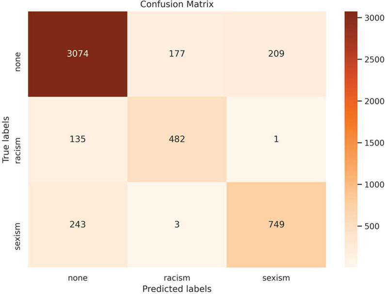
Figure 3 The confusion matrix of the evaluation of the best benchmark model, namely, $M_4$.

As some of them are described in Section 2, there exist various toxic detection studies that utilize different datasets based on different platforms. To benchmark the performance of the proposed model, the related works, that utilized the same dataset as the proposed model, were included in the comparison. As the comparison is listed in Table 12, the proposed model outperformed the related state-of-the-art studies. The plot of the comparison of the related work in terms of obtained classification score is presented in Figure 4.

5 Conclusion

Table 12 The comparison of the proposed work with the related work that utilized the same dataset ($D$) as the proposed model

Related Work	Target Classes	Evaluation Metric	Metric Score
Badjatiya et al. [17]	$racism$, $sexism$, and $none$	Macro averaged $F1-score$	0.73102
Park and Fung [21]	$racism$, $sexism$, and $none$	$F1-score$	$0.8270$
	A combination of $abusive-none$, and $racism-sexism$		$0.8240$
Zhang and Luo [49]	$racism$, $sexism$, and $none$	$F1-score$	$0.8300$
Waseem and Hovy [18]	$racism$, $sexism$, and $none$	$F1-score$	$0.7393$
Agrawal and Awekar [6]	$racism$, $sexism$, and $none$	Macro averaged$F1-score$	$0.7960$${}^2$
Proposed model	$\mathit{r}\mathit{a}\mathit{c}\mathit{i}\mathit{s}\mathit{m}\mathbf{,}\mathit{s}\mathit{e}\mathit{x}\mathit{i}\mathit{s}\mathit{m}$, $\mathit{a}\mathit{n}\mathit{d}\mathit{n}\mathit{o}\mathit{n}\mathit{e}$	Weighted $\mathbf{F1}-\mathit{s}\mathit{c}\mathit{o}\mathit{r}\mathit{e}$	0.8484

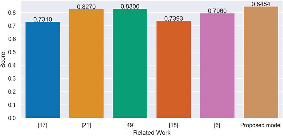
Figure 4 The plot of the comparison of the related work in terms of obtained classification score.

In this study, a novel toxic detection approach based on DNNs was proposed and its efficiency was proven thanks to the conducted experiments. To reveal the most efficient deep neural network model, five widely-used DNNs architectures, namely, ($i$) $CNN$, ($ii$) $LSTM$, ($iii$) $GRU$, ($iv$) $BiLSTM$, and ($v$) a combination of $CNN$ and $BiLSTM$, were investigated. Word embeddings play a critical role in the performance of machine learning models. Therefore, in addition to these DNNs, three widely-used word embedding methods, namely, ($i$) $Word2Vec$, ($ii$) $fastText$, and ($iii$) GloVe, were integrated into the proposed DNNs. As a result of this experimental setup, a total of twenty benchmark models were constructed. These models were evaluated on a gold standard dataset to reveal their efficiency in terms of the detection of toxic posts on social media. According to the experimental result, the proposed $CNN$ model without employing pre-trained word vectors obtained an $F1-score$ of $84.844\%$, which outperformed the related state-of-the-art studies. Other key findings obtained through the conducted experiments are that the models, that constructed word embeddings through the $Embedding$ layers, obtained higher $F1-score$s and converged much faster than the models that utilized pre-trained word vectors. As future work, we would like to cover fine-grained toxicity categories. Also, the proposed novel toxic post detection approach can be applied to posts in other languages. Finally, the networks of the senders of the posts in social media can be investigated to reveal its effect on toxicity detection.

Notes

¹Formspring was later rebranded as Spring.me.

²According to the paper of Arango et al. [19] which takes the methodological issue of this study into account as is briefly discussed in Section 2. Please refer to their paper for more detail regarding this issue.

Acknowledgment

The author would like to thank Waseem and Hovy for sharing their valuable dataset, and Google for providing free resources through the Colab platform.

Funding Information

This research did not receive any specific grant from funding agencies in the public, commercial, or not-for-profit sectors.

References

[1] S. Kemp, “Digital 2020,” We Are Social & Hootsuite, 2020. https://wearesocial.com/digital-2020 (accessed Jan. 29, 2021).

[2] E. Whittaker and R. M. Kowalski, “Cyberbullying Via Social Media,” J. Sch. Violence, vol. 14, no. 1, pp. 11–29, 2015, doi: 10.1080/15388220.2014.949377.

[3] S. Hinduja and J. W. Patchin, “Bullying, Cyberbullying, and Suicide,” Arch. Suicide Res., vol. 14, no. 3, pp. 206–221, 2010, doi: 10.1080/ 13811118.2010.494133.

[4] K. Khieu and N. Narwal, “CS224N: Detecting and Classifying Toxic Comments.”

[5] J. Risch and R. Krestel, “Toxic Comment Detection in Online Discussions,” in Deep Learning-Based Approaches for Sentiment Analysis, Springer, 2020, pp. 1–27.

[6] S. Agrawal and A. Awekar, “Deep Learning for Detecting Cyberbullying Across Multiple Social Media Platforms,” in Proceedings of the Advances in Information Retrieval – 40th European Conference on IR Research (ECIR 2018), 2018, pp. 141–153, doi: 10.1007/978-3-319-76941-7_11.

[7] N. Nandakumar, B. Salehi, and T. Baldwin, “A Comparative Study of Embedding Models in Predicting the Compositionality of Multiword Expressions,” in Proceedings of the Australasian Language Technology Association Workshop 2018 (ALTA 2018), 2018, pp. 71–76.

[8] S. Liu, N. Yang, M. Li, and M. Zhou, “A Recursive Recurrent Neural Network for Statistical Machine Translation,” in Proceedings of the 52nd Annual Meeting of the Association for Computational Linguistics (ACL 2014), 2014, pp. 1491–1500, doi: 10.3115/v1/p14-1140.

[9] D. Tang, F. Wei, N. Yang, M. Zhou, T. Liu, and B. Qin, “Learning Sentiment-Specific Word Embedding for Twitter Sentiment Classification,” in Proceedings of the 52nd Annual Meeting of the Association for Computational Linguistics (ACL 2014), 2014, pp. 1555–1565, doi: 10.3115/v1/p14-1146.

[10] H. Li, X. Li, D. Caragea, and C. Caragea, “Comparison of Word Embeddings and Sentence Encodings as Generalized Representations for Crisis Tweet Classification Tasks,” in Proceedings of the ISCRAM Asian Pacific 2018 Conference, 2018, pp. 1–13.

[11] T. Mikolov, I. Sutskever, K. Chen, G. Corrado, and J. Dean, “Distributed Representations of Words and Phrases and their Compositionality,” in Advances in Neural Information Processing Systems 26: 27th Annual Conference on Neural Information Processing Systems 2013, 2013, pp. 3111–3119.

[12] T. Mikolov, K. Chen, G. Corrado, and J. Dean, “Efficient Estimation ofWord Representations in Vector Space,” in Proceedings of the International Conference on Learning Representations (ICLR 2013), 2013, pp. 1–12.

[13] T. Mikolov, E. Grave, P. Bojanowski, C. Puhrsch, and A. Joulin, “Advances in Pre-Training Distributed Word Representations,” in Proceedings of the 11th International Conference on Language Resources and Evaluation (LREC 2018), 2018, pp. 52–55.

[14] J. Pennington, R. Socher, and C. D. Manning, “GloVe: Global Vectors for Word Representation,” in Proceedings of the 2014 Conference on Empirical Methods in Natural Language Processing (EMNLP 2014), 2014, pp. 1532–1543.

[15] T. Davidson, D. Warmsley, M. Macy, and I. Weber, “Automated Hate Speech Detection and the Problem of Offensive Language,” in Proceedings of the 11th International Conference on Web and Social Media (ICWSM 2017), 2017, pp. 1–4.

[16] Z. Zhang, D. Robinson, and J. Tepper, “Detecting Hate Speech on Twitter Using a Convolution-GRU Based Deep Neural Network,” in Proceedings of the 15th International Conference (ESWC 2018), 2018, pp. 1–15, doi: 10.1007/978-3-319-93417-4_48.

[17] P. Badjatiya, S. Gupta, M. Gupta, and V. Varma, “Deep Learning for Hate Speech Detection in Tweets,” in Proceedings of the 26th International World Wide Web Conference 2017 (WWW ’17 Companion), 2017, pp. 759–760, doi: 10.1145/3041021.3054223.

[18] Z. Waseem and D. Hovy, “Hateful Symbols or Hateful People? Predictive Features for Hate Speech Detection on Twitter,” in Proceedings of the 2016 Conference of the North American Chapter of the Association for Computational Linguistics: Human Language Technologies (NAACL-HLT 2016), 2016, pp. 88–93, doi: 10.18653/v1/n16-2013.

[19] A. Arango, J. Pérez, and B. Poblete, “Hate Speech Detection is Not as Easy as You May Think: A Closer Look at Model Validation,” in Proceedings of the 42nd International ACM SIGIR Conference on Research and Development in Information Retrieval (SIGIR ’19), 2019, pp. 45–54, doi: 10.1016/j.is.2020.101584.

[20] M. Zampieri, S. Malmasi, P. Nakov, S. Rosenthal, N. Farra, and R. Kumar, “Predicting the Type and Target of Offensive Posts in Social Media,” in Proceedings of the 2019 Conference of the North American Chapter of the Association for Computational Linguistics: Human Language Technologies, Volume 1 (Long and Short Papers), 2019, pp. 1415–1420, doi: 10.18653/v1/n19-1144.

[21] J. H. Park and P. Fung, “One-step and Two-step Classification for Abusive Language Detection on Twitter,” in Proceedings of the 1st Workshop on Abusive Language Online to be held at the annual meeting of the Association of Computational Linguistics (ACL) 2017 (ALW1), 2017, pp. 41–45, doi: 10.18653/v1/w17-3006.

[22] C. Van Hee et al., “Automatic detection of cyberbullying in social media text,” PLoS One, pp. 1–22, 2018, doi: 10.17605/OSF.IO/RGQW8.

[23] N. Chakrabarty, “A Machine Learning Approach to Comment Toxicity Classification,” in Proceedings of the 1st International Conference on Computational Intelligence in Pattern Recognition (CIPR 2019), 2019, pp. 1–10.

[24] K. Reynolds, A. Kontostathis, and L. Edwards, “Using machine learning to detect cyberbullying,” in Proceedings of the 2011 10th International Conference on Machine Learning and Applications and Workshops (ICMLA 2011), 2011, pp. 241–244, doi: 10.1109/ICMLA.2011.152.

[25] R. Rehurek and P. Sojka, “Software Framework for Topic Modelling with Large Corpora,” in Proceedings of the LREC 2010 Workshop on New Challenges for NLP Frameworks, 2010, pp. 45–50.

[26] Z. Bairong, W. Wenbo, L. Zhiyu, Z. Chonghui, and T. Shinozaki, “Comparative Analysis of Word Embedding Methods for DSTC6 End-to-End Conversation Modeling Track,” 2017.

[27] S. Hochreiter and J. Schmidhuber, “Long Short-Term Memory,” Neural Comput., vol. 9, no. 8, pp. 1735–1780, 1997, doi: 10.1162/neco.1997.9. 8.1735.

[28] F. Chollet, “Keras: the Python deep learning API,” 2021. https://keras.io (accessed Jan. 29, 2021).

[29] M. Abadi et al., “TensorFlow: A System for Large-Scale Machine Learning,” in Proceedings of the 12th USENIX Symposium on Operating Systems Design and Implementation (OSDI 2016), 2016, pp. 265–283.

[30] F. Chollet, Deep Learning with Python. Manning Publications, 2017.

[31] T. Zhang, W. Zheng, Z. Cui, Y. Zong, J. Yan, and K. Yan, “A Deep Neural Network-Driven Feature Learning Method for Multi-view Facial Expression Recognition,” IEEE Trans. Multimed., vol. 18, no. 12, pp. 2528–2536, 2016, doi: 10.1109/TMM.2016.2598092.

[32] A. Mollahosseini, D. Chan, and M. H. Mahoor, “Going deeper in facial expression recognition using deep neural networks,” in 2016 IEEE Winter Conference on Applications of Computer Vision (WACV 2016), 2016, pp. 1–10, doi: 10.1109/WACV.2016.7477450.

[33] Y. Liu, J. A. Starzyk, and Z. Zhu, “Optimized Approximation Algorithm in Neural Networks Without Overfitting,” IEEE Trans. Neural Networks, vol. 19, no. 6, pp. 983–995, 2008, doi: 10.1109/TNN.2007.915114.

[34] V. Nair and G. E. Hinton, “Rectified Linear Units Improve Restricted Boltzmann Machines,” in Proceedings, of the 27th International Conference on Machine Learning (ICML 2010), 2010, pp. 807–814.

[35] J. Xiong, K. Zhang, and H. Zhang, “A Vibrating Mechanism to Prevent Neural Networks from Overfitting,” in Proceedings of the 2019 15th International Wireless Communications and Mobile Computing Conference (IWCMC 2019), 2019, pp. 1737–1742, doi: 10.1109/IWCMC.2019.8766500.

[36] H. Wang, Y. Zhang, and X. Yu, “An Overview of Image Caption Generation Methods,” Comput. Intell. Neurosci., vol. 2020, pp. 1–13, 2020, doi: 10.1155/2020/3062706.

[37] A. Graves and J. Schmidhuber, “Framewise phoneme classification with bidirectional LSTM and other neural network architectures,” Neural Networks, vol. 18, no. 2005 Special Issue, pp. 602–610, 2005, doi: 10.1016/j.neunet.2005.06.042.

[38] W. Wang and B. Chang, “Graph-based Dependency Parsing with Bidirectional LSTM,” in Proceedings of the 54th Annual Meeting of the Association for Computational Linguistics (ACL 2016), 2016, pp. 2306–2315, doi: 10.18653/v1/p16-1218.

[39] D. P. Kingma and J. L. Ba, “Adam: A Method for Stochastic Optimization,” in Proceedings of the 3rd International Conference on Learning Representations (ICLR 2015), 2015, pp. 1–15.

[40] H. Robbins and S. Monro, “A Stochastic Approximation Method,” Ann. Math. Stat., vol. 22, no. 3, pp. 400–407, 1951, doi: 10.1214/aoms/1177729586.

[41] B. Wu, Z. Liu, Z. Yuan, G. Sun, and C. Wu, “Reducing Overfitting in Deep Convolutional Neural Networks Using Redundancy Regularizer,” in 26th International Conference on Artificial Neural Networks (ICANN 2017), 2017, pp. 49–55, doi: 10.1007/978-3-319-68612-7_6.

[42] X. Ying, “An Overview of Overfitting and its Solutions,” in Proceedings of the International Conference on Computer Information Science and Application Technology (CISAT 2018), 2018, pp. 1–6, doi: 10.1088/1742-6596/1168/2/022022.

[43] R. F. Liao, H. Wen, J. Wu, H. Song, F. Pan, and L. Dong, “The Rayleigh Fading Channel Prediction via Deep Learning,” Wirel. Commun. Mob. Comput., vol. 2018, pp. 1–11, 2018, doi: 10.1155/2018/6497340.

[44] “Tweepy,” 2021. https://www.tweepy.org (accessed Jan. 29, 2021).

[45] J. Camacho-Collados and M. T. Pilehvar, “On the Role of Text Preprocessing in Neural Network Architectures: An Evaluation Study on Text Categorization and Sentiment Analysis,” in Proceedings of the 2018 EMNLP Workshop BlackboxNLP: Analyzing and Interpreting Neural Networks for NLP, 2018, pp. 40–46, doi: 10.18653/v1/w18-5406.

[46] S. Bird, E. Klein, and E. Loper, Natural Language Processing With Python, 1st ed. O’Reilly Media, 2009.

[47] M. Pumperla, “Hyperas by maxpumperla,” 2021. http://maxpumperla.com/hyperas/ (accessed Jan. 29, 2021).

[48] “Colaboratory,” Google, 2021. https://colab.research.google.com (accessed Jan. 29, 2021).

[49] Z. Zhang and L. Luo, “Hate Speech Detection: A Solved Problem? The Challenging Case of Long Tail on Twitter,” Semant. Web, vol. 1, no. 0, pp. 1–21, 2018.

Biography

Abdullah Kabakus received the bachelor’s degree in computer engineering from Cankaya University in 2010, the master’s degree in computer engineering from Gazi University in 2014, and the philosophy of doctorate degree in Electrical-Electronics & Computer Engineering from Duzce University in 2017, respectively. He is currently working as an Associate Professor at the Department of Computer Engineering, Faculty of Engineering, Duzce University. His research areas include mobile security, deep learning, and social network analysis. He has been serving as a reviewer for many highly-respected journals.

Journal of Web Engineering, Vol. 20_8, 2243–2268.
doi: 10.13052/jwe1540-9589.2082
© 2021 River Publishers

Abstract

1 Introduction

2 Related Work

3 Material and Method

3.1 Word Embedding Methods

3.1.1 Word2Vec

3.1.2 GloVe

3.1.3 fastText

3.2 Proposed Deep Neural Network Models

3.2.1 Proposed CNN model

3.2.2 Proposed LSTM Model

3.2.3 Proposed GRU model

3.2.4 Proposed BiLSTM model

3.2.5 Proposed CNN$+$BiLSTM model

3.3 Training Configuration

3.4 Data Preparation

3.5 Model Optimization

4 Experimental Result and Discussion

5 Conclusion

Notes

Acknowledgment

Funding Information

References

Biography