Research on Data Release and Location Monitoring Technology of Sensor Network Based on Internet of Things

Bin Lin

School of Optical-Electrical and Computer Engineering, University of Shanghai for Science and Technology, Shanghai 200093, China

E-mail: Linbin2021@163.com

Received 18 March 2021; Accepted 23 April 2021; Publication 02 June 2021

Abstract

The Internet of Things is another information technology revolution and industrial wave after computer, Internet and mobile communication. It is becoming a key foundation and an important engine for the green, intelligent and sustainable development of economic society. The new networked intelligent production mode characterized by the integration innovation of the Internet of Things is shaping the core competitiveness of the future manufacturing industry. The application of sensor network data positioning and monitoring technology based on the Internet of Things in industry, power and other industries is a hot field for the development of the Internet of Things. Sensor network processing and industrial applications are becoming increasingly complex, and new features have appeared in the sensor network scale and infrastructure in these fields. Therefore, the Internet of Things perception data processing has become a research hotspot in the deep integration process between industry and the Internet of Things. This paper deeply analyzes and summarizes the characteristics of sensor network perception data under the new trend of the Internet of Things as well as the research on location monitoring technology, and makes in-depth exploration from the release and location monitoring of sensor network perception data of the Internet of Things. Sensor network technology integrated sensor technology, micro-electromechanical system technology, wireless communication technology, embedded computing technology and distributed information processing technology in one, with easy layout, easy control, low power consumption, flexible communication, low cost and other characteristics. Therefore, based on the release and location monitoring technologies of sensor network data based on the Internet of Things in different applications, this paper studies the corresponding networking technologies, energy management, data management and fusion methods. Standardization system in wireless sensor network low cost, and convenient data management needs, design the iot oriented middleware, and develops the software and hardware system, the application demonstration, the results show that the design of wireless sensor network based on iot data monitoring and positioning technology is better meet the application requirements, fine convenient integration of software and hardware, and standardized requirements and suitable for promotion.

Keywords: Internet of Things sensor network, data location monitoring technology, WSNs location algorithm, Huffman coding, industrial systems monitor the Internet of Things.

1 Introduction

Urban lifeline security operation monitoring system is an urban scale disaster monitoring network, which realizes the overall safety monitoring, early warning and rapid response to important urban infrastructure. In recent years, China’s Internet of Things related industries and technology applications have developed rapidly. Especially in the field of urban management, water supply, drainage, gas, heat and electricity are important infrastructure and organic components of urban lifeline, and guarantee to maintain urban life and production. It is urgent to apply Internet of Things technology to real-time monitoring of urban operation signs, improve the management level of urban lifeline and the ability of prevention, prediction and disposal, and guarantee the safe and stable operation of the city [1]. Research on sensor network data release and location monitoring technology based on The Internet of Things, starting from analyzing the current situation and main problems of urban lifeline management; Combining the development of the Internet of Things and its key technologies; With the application demonstration of urban lifeline real-time monitoring Internet of Things as the research background, the key technologies of sensor network data processing layer algorithm, sensor node position algorithm and algorithm accuracy improvement are studied. The network architecture of the Internet of Things consists of the perception layer, the network layer and the application layer. The sensor network processing of the Internet of Things runs through the whole network architecture [2]. At present, the Internet of things of sensor network processing research focused on the Internet of things application layer, using the sensor network data for high performance computing, artificial intelligence, database and fuzzy computing technology, such as general perception of collecting data processing, mainly related to parallel computing, data mining, platform service, information, etc. Through the collection of sensor network data, high performance computing is carried out so as to accurately locate and monitor the management of urban lifeline and other important projects. Intelligent processing and analysis of the collected perception data can also form a variety of applications with commercial value [3]. We need to digitize the complex systems, through the sensor network, monitoring and intelligent recognition based database of urban lifeline, establish a highly intelligent directly for urban lifeline running management, positioning detection, emergency support and leadership decision-making information sharing and exchange, to grasp the resource planning, scheduling, inventory demand operation information, such as the analysis and synthesis, wireless location technology is based on measuring the parameters of the radio waves, combined with specific localization algorithm to calculate the location information of object to be tested. It includes infrared, ultrasonic, Bluetooth, RADIO frequency identification, ultra-wideband, WIFI, Zidbee, etc., and was originally designed to meet the needs of long-distance navigation and navigation [4]. Wireless positioning resolution can be accurate to 0.25 m, which is widely used in mobile phone user positioning, mine personnel positioning, disaster site personnel search and rescue, container transport tracking, vehicle navigation and other aspects. In WSNs, in addition to reporting the location of detected events, location information can also be used for target tracking, assisting in routing and network topology management, etc. The European Telecommunications Standardization Association ETSI has developed a series of standards for the wireless positioning of GSM system. At present, the mobile positioning service industry has become one of the most potential mobile value-added services. In general, under the limited conditions of current sensor equipment and positioning system, efforts are made to achieve the most efficient and effective positioning method. Figure 1 illustrates a positioning problem, and it should be noted that a generic node can also be used as an anchor node, as long as it knows its location [5].

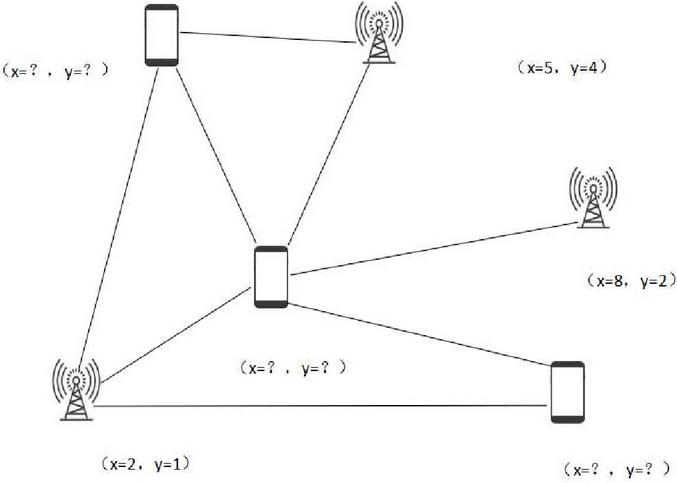
Figure 1 Anchor node location problem.

In the WSNs positioning algorithm selected in this paper, the positioning accuracy is generally expressed by the ratio of the error value to the wireless range of the node. In addition, some positioning algorithms use the size of the two-dimensional network to express its accuracy. Another important indicator of the merits of WSNs positioning algorithm is the density of reference nodes [6]. Due to human or using GPS in WSN way to deploy the reference node has a great influence on the environment and WSNs applications extensibility are, therefore, the reference node density can be used to evaluate location of one of the important indices for monitoring cost and scalability of the algorithm through the sensor network positioning monitoring data, the overall operation to provide effective services, enhancing the management level of safe operation. When the performance index of WSNs positioning algorithm is used for analysis, generally a better positioning algorithm should be characterized by high accuracy, low reference node dependence, strong fault tolerance and robustness, as well as low energy consumption and implementation cost. These performance indexes are not only the performance indexes to evaluate WSNs’ own positioning algorithm, but also the optimal objectives for its positioning algorithm research and design. In WSNs positioning, it is often necessary to comprehensively consider these performance indicators and make tradeoffs according to specific requirements, and propose positioning algorithms applied to different scenarios and standards [7]. As the basic unit of network, sensor node is generally composed of data acquisition module, processing module, wireless communication module and energy supply module, as shown in the figure. Sensor nodes are mainly responsible for data acquisition and preprocessing, and respond to data transmission according to the instructions of the monitoring center. Currently, most energy supply modules use batteries. The deployment of nodes can be randomly distributed in the monitored area, and the network can be formed in the form of self-organization. The location of each node can be determined by positioning or by virtue of node self-positioning algorithm [8, 9].

2 Algorithm Research

2.1 Sensor Network Data Processing Layer Algorithm

In the architecture design of middleware sensor for Internet of Things application, the data processing layer will process the data returned by the data acquisition layer, and the data compression component will compress and process the historical data collected, so as to save the initial data returned by the acquisition layer for redundant operation. Because the objects of urban lifeline real-time monitoring have the characteristics of wide location distribution, great quantity, great quantity and frequent sampling. In the transmission process of system data, due to the variety of real-time data, complex sources, fast update speed and high precision requirements, the amount of historical data to be saved is very large [10–12]. If these data are stored directly, it will take up a lot of storage space, and it will also backup the data transmission and publish historical data. The data compression component is a very important part of the sensor network data processing layer. It is mainly a common compression method used to publish and monitor network data. The lossless compression method based on statistics is based on variable-length coding theory, which is the most widely used compression method at present. By assigning the probability of each symbol in the source, Huffman code assigns the code word with the lowest probability, and the symbol with the higher probability, the code word with the shorter, so as to use as few code symbols as possible to represent the source data and achieve the effect of compression [13].

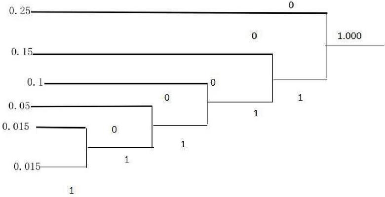
Figure 2 Huffman Coding process.

Another limit of Huffman coding is invalid, or if a source consists of two symbols can only assign the 0 s and 1 s two code word for two symbols, the average code length is 1, if the two symbols appear probability vary widely, coding efficiency will be very low, coding have solved this problem, this method broke this restriction, it took a long code word assigned to the input stream, not for sensor source distribution for each symbol of the code word it according to the probability of the emergence of the symbol sequence of several linear interval segmentation, and says it has split range of binary decimal code as the corresponding sequence [14]. The algorithm simplifies the revolving door algorithm by setting some rules, which avoids the storage of a large amount of temporary data, thus improving the efficiency of the algorithm and reducing the time complexity. However, there are two parameters in the algorithm that need to be set: compression deviation value and filtering value. If the setting of the compression deviation value is too small, it will affect the release rate of data, while if the setting is too large, it will affect the data release rate [15].

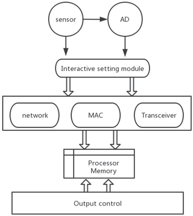
Figure 3 Sensor node structure diagram.

As shown in Figure 3, the cluster is a concept closely related to the sensor node in the sensor network, which is composed of several adjacent sensor nodes in the network, and one node is selected as the cluster head in each cluster. The formation of clusters and the selection of cluster heads usually depend on the cluster algorithm used in the network. Convergent nodes, commonly known as gateways, are mainly responsible for collecting data from clusters [16]. Convergent nodes can not only be connected to the network, but also directly to the task management node. The cluster data is transmitted to the convergent node by “multi-hop” routing, and the convergent node sends the data to the task management node, thus completing the information interaction between the sensor node and the task management node. The field information collected by sensor node is transmitted to task management node to realize site location monitoring. In addition, task manager has an important role, that is, it can manage the sensor nodes in the whole network and publish the data.

2.2 Algorithm Processing

Step 1: Determine the initial range of the two parameters

First, the absolute value difference between the historical data values is calculated, and the minimum value and the maximum value are selected as follows

As shown in the formula, the initial value range of the two parameters can be defined as:

$\xi \in (\mathrm{m},\mathrm{r}),\epsilon \in (\mathrm{l},\mathrm{m})$
$\{\begin{array}{c}\mathrm{l}=\min |{\mathrm{y}}_{\mathrm{n}}-{\mathrm{y}}_{\mathrm{n}-1}|\hfill \\ \mathrm{r}=\max |{\mathrm{y}}_{\mathrm{n}}-{\mathrm{y}}_{\mathrm{n}-1}|\hfill \\ \mathrm{m}=\mathrm{median}|\mathrm{yn}-\mathrm{yn}-1|\hfill \end{array}$	(1)

Step 2: coding, there are many suitable coding methods, choose the most commonly used quaternary coding, using 2-bit quaternion coding, respectively to represent the corresponding compression deviation and filter value size [17].

Step 3: fitness function, in the process of algorithm optimization, a good fitness function can guide the direction of optimization. Previously mentioned data compression technology includes two key technologies, data compression ratio and data decompression performance. The decompression algorithm corresponds to the compression algorithm used. The usual decompression algorithm is linear interpolation, as follows:

$$\widehat{\mathrm{y}}={\mathrm{y}}_0+\frac{{\mathrm{y}}_{\mathrm{n}}-{\mathrm{y}}_0}{{\mathrm{t}}_{\mathrm{n}}-{\mathrm{t}}_0}(\mathrm{t}-{\mathrm{t}}_0)$$

(2)

In order to ensure the performance of the algorithm and reduce the error caused by the decompression of the network data obtained by the sensor, the error of the network data release can be reduced. The fitness function is defined as follows:

$$\mathrm{Fitness}=1/\sqrt{\frac{1}{\mathrm{n}}\sum _{\mathrm{j}=1}^{\mathrm{n}}({\mathrm{y}}_{\mathrm{j}}-{\mathrm{y}}_{\mathrm{j}}^2)}$$

(3)

The fitness function represents the reciprocal of the compression error, and the larger the value, the better the effect of data release. An individual i is selected with the following probabilities:

$$\mathrm{Pi}=\mathrm{fi}/\sum _{\mathrm{i}=1}^{\mathrm{ps}}{\mathrm{f}}_{\mathrm{i}}$$

(4)

Step 4: stop condition, this paper sets the number of iterations as the algorithm stop condition. When the preset iteration number is reached and the algorithm ends, the output optimal individual is the optimal result of two parameters.

The encoded compressed matrix is shown in Figure 4.

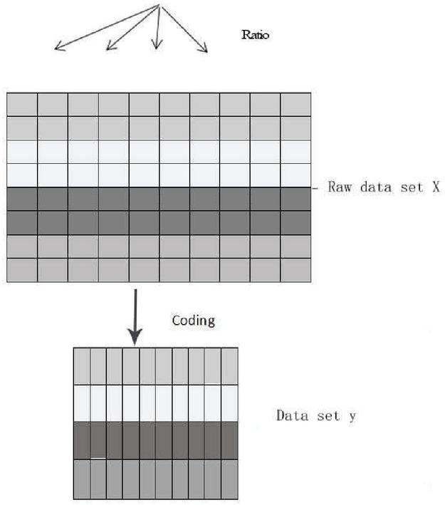
Figure 4 Compression algorithm matrix.

The process of data dissemination is:

1. uniformly split x by rows into $m$ subspaces

2. broadcast model to all nodes

3. $n\leftarrow num$ of columns of x

4. FOREACH subspace $i=1$; $m$, column $j=1$ n in parallel DO

5. $y[i,j]\leftarrow$ model [I] predict ($x$[i, j])

6. END FOREACH

7. RETURN y

2.3 Location Algorithm of Internet of Things Sensor Node

There are n sensors in the Internet of things grid, which periodically monitor the surrounding environment for data acquisition. The IED node is located in the center of the region, and the network can cover all the monitoring areas. Let CI represent the i sensor node, then the node set is:

$$C=\{{\mathrm{C}}_{\mathrm{i}}|\mathrm{l}\le \mathrm{i}\le \mathrm{n}\}$$

(5)

The energy consumption of the node to send X bit data to a d distance is:

$$ET\mathrm{x}(\mathrm{l},\mathrm{d})=\left\{\begin{array}{cc}\mathrm{l}{E}_{\mathrm{elec}}+\mathrm{l}{\epsilon }_{\mathrm{fs}}{\mathrm{d}}^2,\hfill & \mathrm{d}<{\mathrm{d}}_0\hfill \\ \mathrm{l}{E}_{\mathrm{elec}}=\mathrm{l}{\epsilon }_{\mathrm{mp}}{\mathrm{d}}^4,\hfill & \mathrm{d}\ge {\mathrm{d}}_0\hfill \end{array}\right\}$$

(6)

The energy consumption of nodes receiving l bits of data is:

$$E_{R\mathrm{x}}(\mathrm{l})=\mathrm{l}{E}_{\mathrm{elec}}$$

(7)

In the Internet of things based sensing network, the sensor nodes are distributed unevenly, and the sensing nodes are randomly distributed in the monitoring area. The distribution of the sensor node relay nodes and the computing nodes is shown in Figure 5.

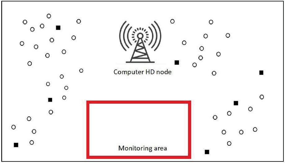
Figure 5 Select the distribution of sensor sensing network nodes in the monitoring area.

The code attempts to:

1. FOR $i=1\to m$ DO

2. FOR $j=1\to$ model[i], num Of Centers

3. $D[i,j]\leftarrow$ compute Dist (model[i], center[j], q)

4. END FOR

5. END FOR

6. n $\leftarrow$ num of columns of y

7. broadcast dist to all nodes

8. FOREACH subspace $\mathrm{i}=1$; m, column $\mathrm{j}=1$ n in

9. dist [i] $\leftarrow$ dist[i] $+$ D[i, y[i, j]]

10. END FOREACH

11. result $\leftarrow$ get TopK (dist)

12. RETURN result

Combined with the code, the nodes in a monitoring area are divided into several clusters based on density, and each cluster is selected in parallel. Figure 6 is a cluster diagram of a grid.

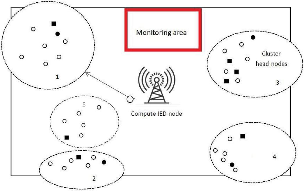
Figure 6 Select the schematic diagram of sensor node clustering in the monitoring area.

3 Improved Accuracy of the Algorithm

Because of the limited computing power and storage space of Internet of things wireless sensor network nodes, this paper adopts linear regression model, which improves the prediction accuracy and reduces the complexity of the algorithm. In the form of:

$${\mathrm{x}}^{\prime }=\mathrm{x}+\mathrm{yt}$$

(8)

The collection of n sensing data sampled by nodes in the Internet of things wireless sensor network in chronological order is recorded as:

$$TS=\{({\mathrm{t}}_1,{\alpha }_1),({\mathrm{t}}_2,{\alpha }_2),\mathrm{\dots },({\mathrm{t}}_{\mathrm{n}},{\alpha }_{\mathrm{n}})\}$$

(9)

In order to minimize the sum of squares between sampling data and error, is shown as:

$$D=\sum _{\mathrm{i}=1}^{\mathrm{n}}{\mathrm{D}}_{\mathrm{i}}^2=\sum _{\mathrm{i}=1}^{\mathrm{n}}{[{\alpha }_{\mathrm{i}}-(\mathrm{x}+{\mathrm{yt}}_{\mathrm{i}})]}^2$$

(10)

Then the network energy consumption is:

$EC(R)$	$={\mathrm{p}}_{0\mathrm{proc}}({\mathrm{t}}_{0^{\prime }\mathrm{setup}}+{\mathrm{t}}_{0^{\prime }\mathrm{acq}}+{\mathrm{t}}_{0^{\prime }\mathrm{proc}})+{\mathrm{p}}_{0^{\prime }\mathrm{tran}},{\mathrm{t}}_0,{\mathrm{t}}_{\mathrm{ran}}$
	$\mathrm{\hspace{1em}}+{\displaystyle \sum _{\mathrm{k}=1}^{H-1}}\{{\mathrm{p}}_{\mathrm{k}},\mathrm{proc}+({\mathrm{t}}_{{\mathrm{k}}^{\prime }\mathrm{proc}})\}$	(11)

The network packet loss rate is:

$$\mathrm{p}-\mathrm{loss}(\mathrm{p}({\mathrm{v}}_{\mathrm{s}},{\mathrm{v}}_{\mathrm{d}}))=\frac{\mathrm{loss}(\mathrm{e})}{\mathrm{packet}(\mathrm{p}({\mathrm{v}}_{\mathrm{s}},{\mathrm{v}}_{\mathrm{d}}))}$$

(12)

In order to solve the problems in practical application and improve the positioning accuracy. Assuming that the unknown node is A, from each beacon node, the weighted value of the average hop distance of each wrong node is recorded as

$$A_{\mathrm{i}}=\frac{\frac{1}{\mathrm{h}}}{{}_{\mathrm{i}=1}{}^{\mathrm{n}}\left(\frac{1}{\mathrm{h}}\right)}$$

(13)

Correction of distance values:

$${\mathrm{correction}}_{\mathrm{ij}}=\frac{(H_{\mathrm{i},\mathrm{f}}({\mathrm{Hopsize}}_{\mathrm{i}}{\mathrm{Dis}}_{\mathrm{i},\mathrm{j}})/H_{\mathrm{i},\mathrm{j}})}{{\mathrm{Dis}}_{\mathrm{i},\mathrm{j}}}$$

(14)

Final correction distance:

$$\mathrm{dis}{\mathrm{Corr}}_{\mathrm{k},\mathrm{i}}=\frac{{\mathrm{dis}}_{\mathrm{k},\mathrm{i}}}{1+{\mathrm{Correction}}_{\mathrm{k},\mathrm{i}}{\mathrm{h}}_{\mathrm{k},\mathrm{i}}}$$

(15)

A weighting factor is introduced into each set of positioning coordinates. The weighted factor is obtained by participating in the radius of each location area. The calculation formula is as follows:

$\mathrm{A}E$	$={\displaystyle \frac{\frac{\mathrm{A}{E}_1}{{\mathrm{r}}_B+{\mathrm{r}}_C+{\mathrm{r}}_E}+\frac{\mathrm{A}{E}_2}{{\mathrm{r}}_A+{\mathrm{r}}_B+{\mathrm{r}}_D}+\frac{\mathrm{A}{E}_3}{{\mathrm{r}}_A+{\mathrm{r}}_B+{\mathrm{r}}_D}+\frac{\mathrm{A}{E}_4}{{\mathrm{r}}_A+{\mathrm{r}}_{\mathrm{c}}+{\mathrm{r}}_E}+\frac{A{E}_5}{{\mathrm{r}}_C+r_D+r_E}}{\frac{1}{{\mathrm{r}}_A+{\mathrm{r}}_B+{\mathrm{r}}_C}+\frac{1}{{\mathrm{r}}_A+{\mathrm{r}}_B+{\mathrm{r}}_E}+\frac{1}{{\mathrm{r}}_E+{\mathrm{r}}_{\mathrm{c}}+{\mathrm{r}}_D}+\frac{1}{{\mathrm{r}}_B+{\mathrm{r}}_C+{\mathrm{r}}_D}+\frac{1}{{\mathrm{r}}_D+r_E+r_A}}}$	(16)
$\mathrm{B}E$	$={\displaystyle \frac{\frac{\mathrm{B}{E}_1}{{\mathrm{r}}_B+{\mathrm{r}}_C+{\mathrm{r}}_E}+\frac{\mathrm{B}{E}_2}{{\mathrm{r}}_A+{\mathrm{r}}_B+{\mathrm{r}}_D}+\frac{\mathrm{B}{E}_3}{{\mathrm{r}}_A+{\mathrm{r}}_B+{\mathrm{r}}_D}+\frac{\mathrm{B}{E}_4}{{\mathrm{r}}_A+{\mathrm{r}}_{\mathrm{c}}+{\mathrm{r}}_E}+\frac{B{E}_5}{{\mathrm{r}}_C+r_D+r_E}}{\frac{1}{{\mathrm{r}}_A+{\mathrm{r}}_B+{\mathrm{r}}_C}+\frac{1}{{\mathrm{r}}_A+{\mathrm{r}}_B+{\mathrm{r}}_E}+\frac{1}{{\mathrm{r}}_E+{\mathrm{r}}_{\mathrm{c}}+{\mathrm{r}}_D}+\frac{1}{{\mathrm{r}}_B+{\mathrm{r}}_C+{\mathrm{r}}_D}+\frac{1}{{\mathrm{r}}_D+r_E+r_A}}}$	(17)

A, B in the above formula is the final positioning coordinate.

4 Internet of Things Positioning Monitoring System Positioning Technology

As shown in Figure 7, In the positioning process of iot positioning monitoring system, the gateway first sends anchor node initialization information wirelessly, and all anchor nodes in the management area are initialized [18]. Then, the mobile unknown node is sent to initialize the request, and after the initialization of the mobile unknown node is completed, the unicast mobile node sends the reply information. The mobile node broadcasts the RSSI request message to the reference node, obtains coordinates and signal strength information of all reference nodes within one hop range, calculates its own position, and sends it to the gateway packaged [19].

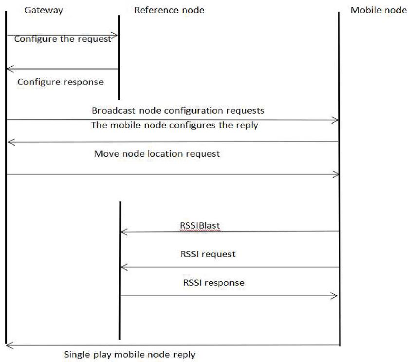
Figure 7 Positioning process diagram of iot positioning monitoring system.

As shown in Figure 8, the positioning engine is a device to calculate the position of the mobile node. Its basic principle is to calculate the positioning based on the coordinate value of the reference node and the signal strength between the obtained and the reference node. The positioning engine input coordinates and signal strength values of four reference nodes at a time, and input coordinates and information strength values of six reference nodes at a time for calculation. Write the reference coordinates and the measurement parameters. After obtaining the effective location information of anchor nodes, the algorithm also needs auxiliary measurement parameters to complete the positioning calculation of unknown nodes. This set of parameters includes 2 environmental measurement parameters A and N and 6 signal strength values obtained from reference nodes. When writing these parameters, you also need to identify position 1 and write to the positioning engine once [20–22].

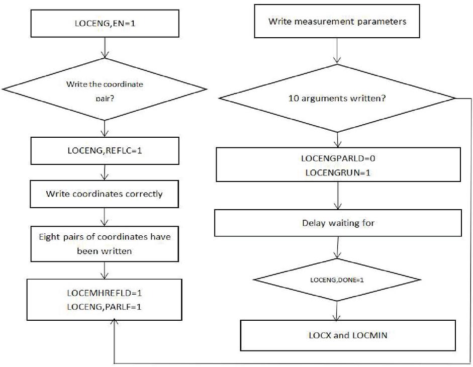
Figure 8 The flow chart of the positioning process of the iot positioning monitoring system.

5 Performance Tests

This experiment looks for positioning monitoring technology for urban open space location test, because the final scheme adopted in this paper is the positioning effect in the case of outdoor open space. The test environment is to ensure that there are no obstacles in the open space. The number of reference nodes considers two cases, one with 4 anchor reference nodes and the other with 6 anchor reference nodes. The specific area tested is within the plane range of 6 m $\times$ 6 m. In the case of 4 anchor nodes, take 4 vertices of the plane region; in the case of 6 anchor nodes, take 6 anchor reference nodes of the plane region. 6 unknown nodes are randomly placed, namely 6 unknown locations. The specific location information is shown in Table 1. The transmitting power of the nodes is set to 0dbm, and the nodes are all in a plane height. Both the anchor reference node and the unknown node adopt the whip antenna, the antenna square to make the RF signal to transmit outward and upward [23].

Table 1 Measurement results

Four Reference Nodes		SIX Reference Nodes
Actual	Node	Actual	Node
Node	Measuring	Node	Measuring
Coordinates (A,B)	Coordinates (A,B)	Coordinates (A,B)	Coordinates (A,B)
(2.2,2.3)	(2.5,3.6)	(2.2,2.3)	(0.5,2.8)
(2.4,6.6)	(4.4,5.6)	(2.4,6.6)	(3.7,6.2)
(4.3,4.4)	(2.3,5.6)	(4.3,4.4)	(5.3,5.2)
(6.7,2.7)	(8.7,0.9)	(6.7,2.7)	(5.8,2.2)
(6.4,7.2)	(5.4,6.5)	(6.4,2.7)	(5.8,2.2)
(9.8,2.4)	(22.8,4.5)	(9.8,2.4)	(22.2,4.0)
(8.8,4.4)	(6.8,7.5)	(8.8,4.4)	(20.4,6.3)

According to the performance analysis of the test results above, with the increase of the number of reference anchor nodes in the network, the distance error of the nodes will decrease accordingly. The error difference between the four anchor nodes and the six anchor nodes is obvious. In addition, in the region formed by 6 m $\times$ 6 m anchor nodes, the corresponding distance error is significantly lower than that outside the region of 6 m$\times$ 6 m. In the actual test, the local node sends a command to the remote node to initialize the test, and then repeats the test described above for many times. The layout and hardware structure are shown in Figure 10. Finally, the local node requests the packet containing the ranging results to the remote node, and the remote node sends the test result data to the local node after receiving the request. Over short distances, the TOF measurement results are negative [24]. Therefore, the ranging scheme is introduced in the short-distance ranging process, after a lot of specific experiments. It is learned that the RSSI value can be used to monitor different nodes, and the monitoring system flow built is shown in Figure 9. However, as the RSSI value and distance are inversely square, the farther the distance is, the more inaccurate the RSSI method is. In general, the RSSI method is accurate when the distance is less than about 19 m. RSSI ranging is used, and the RSSI and range model are important. Below are the solutions of RSSI and TOF respectively.

$T_{TOF}$	$={\displaystyle \frac{T_{RTT}}{2}}={\displaystyle \frac{T_{TOT}-T_{TAT}}{2}}$
$\mathrm{range}$	$=0.02\times {10}^{(\frac{108-RSSI}{19})}$	(18)

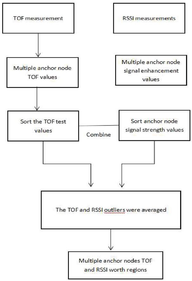
Figure 9 Internet of things location monitoring system monitoring and construction process.

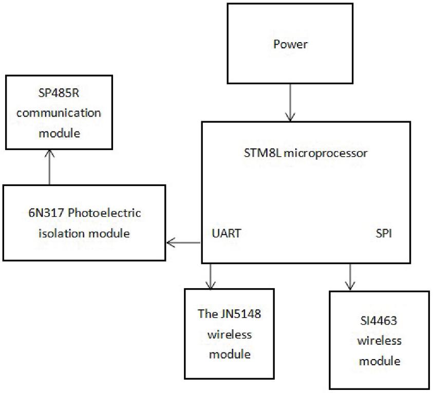
Figure 10 Layout and hardware structure of iot positioning monitoring system.

6 Inspection Analysis

In order to verify the effect of the Internet of Things positioning monitoring data compression algorithm mentioned in this paper, the synthetic data are simulated, the performance of the method is analyzed and compared, and the sine wave amplitude and sampling accuracy are considered comprehensively. At the same time, noise N(t) is superimposed on the data. N(t) is a random number whose value range is $[-0.65,0.65]$. Table 2 lists the simulation results of synthetic data, where the record limit of the traditional algorithm is 2.

Table 2 Simulation results

Data	Compression Algorithm	Compression Ratio	Compression Error
Data 1	SDT	4.99	2665.42
	ISDT	6.02	2602.92
Data 2	SDT	9.95	2566.22
	ISDT	22.39	2490.95

The results in Table 3 show that the proposed algorithm can effectively improve the performance of the traditional algorithm. From the point of view of the ratio of compressed published data, the algorithm in this paper increases by about 20% compared with the traditional algorithm, while the error is reduced by about 5% on average. This shows that the improved sensor network data publishing and positioning algorithm based on the Internet of things can effectively improve the compression effect and verify the feasibility of the method.

Table 3 Experimental recall rates for the number of different nodes

	The Recall	The Recall	The Recall	The Recall	The Recall	The Recall
Node	Rate	Rate	Rate	Rate	Rate	Rate
Values	(R $=$ 2)	(R $=$ 5)	(R $=$ 20)	(R $=$ 20)	(R $=$ 50)	(R $=$ 200)
2	0.226	0.330	0.482	0.604	0.846	0.929
2	0.232	0.329	0.469	0.602	0.855	0.923
3	0.220	0.322	0.464	0.600	0.849	0.922
4	0.224	0.329	0.466	0.593	0.854	0.922

As can be seen only from Table 3, the recall rates of the experiments on sensor cluster systems with different number of nodes differ little. In ensuring the recall rate under the condition of little change, from the table we can see in training, code, and query on the three stages of time consumption, increase in the number of nodes, training time drops rapidly and gradually slow, did not keep the ideal linear downward trend, this is due to the increase in the number of additional computational overhead increases when the cluster nodes, including network communication time, etc. On the whole, the time consumption decreases with the increase of nodes, which indicates that the algorithm system has good scalability. In addition, the relationship between the size of the training set and the training time is also tested on the data set collected by the sensor [25]. By changing the size of different training data sets, the recall rate and time consumption of experiments are compared to verify the scalability of the algorithm. In terms of experimental parameter setting, we used the same configuration as the cluster experiment in the previous experiment. Similarly, we use recall rate as a standard to measure the quality of query results. For differences, the training set sizes were 0.1 m, 0.2 m, 0.5 m and 1 M respectively for experiments, and the changes of experimental recall rate and time consumption were observed. Table 4 shows that when the size of the training set in the experiment is changed, the recall rate shows an increasing trend with the increase of the training set, but it is not obvious. From Table 5, we can see that with the increase of training set, the training time increases rapidly and then gradually increases slowly. The encoding time and the time for a single query change little because they are not affected by the size change of the training data set. Therefore, the experiment shows that the localization monitoring system has good scalability.

Table 4 Experimental recall of data size of different training sets

Training	Recall	Recall	Recall	Recall	Recall	Recall	Recall
Set	Rate	Rate	Rate	Rate	Rate	Rate	Rate
Size/M	(R $=$ 2)	(R $=$ 2)	(R $=$ 5)	(R $=$ 20)	(R $=$ 20)	(R $=$ 50)	(R $=$ 200)
0.1	0.224	0.329	0.466	0.593	0.623	0.854	0.922
0.2	0.223	0.322	0.469	0.596	0.629	0.826	0.924
0.5	0.222	0.323	0.463	0.600	0.626	0.859	0.924
1.0	0.222	0.326	0.462	0.603	0.626	0.855	0.926

Table 5 Experimental time of data size of different training sets

Training Set/M	Training Time/s	Encoding Time/s	Single Query/s
0.1	542.3	5.08	2.49
0.2	2235.6	5.22	2.48
0.5	2602.5	5.28	2.46
1.0	5626.3	4.93	2.46

7 Conclusion

This paper has realized a set of positioning monitoring system applied in sensor network technology of the Internet of Things and based on the Internet of Things, which can be used for monitoring personnel to implement layout monitoring at any time. This paper studies the problem of approximate neighbor query and location in the large-scale high-dimensional data publishing of sensors in the Internet of Things. Through the in-depth discussion of the hash method of product quantization, a set of approximate neighbor query system based on distributed hash algorithm is implemented on the sensor platform and technology of the Internet of Things. On the one hand, the system can compress and encode the sensor data, which can greatly reduce the space occupation. On the other hand, while ensuring the accuracy of query, the parallel computing of cluster system can greatly improve the efficiency of query. Through the key technology research of Internet of Things for urban monitoring in this paper, the design realization, smooth implementation and reliable operation of the project are guaranteed. At the same time, the practical application of these research results in the application demonstration system of urban monitoring Internet of things can improve the technical level of urban lifeline monitoring and management, which has important application value and practical significance, and will promote the development of urban lifeline management towards digitalization, precision and intelligence.

References

[1] Y. Zhang, L. Sun, J. Liu, et al., “Design and implementation of intelligent art lighting systems based on wireless sensor network technology,” in 2011 Chinese Control and Decision Conference (CCDC), Mianyang, China, 2011, pp. 3765–3770.

[2] B. Koo, H. Choi, and T. Shon, “WIVA: WSN monitoring framework based on 3D visualization and augmented reality in mobile devices,” in International Conference Smart Homes and Health Tlematics, Tours, France, 2009, pp. 158–165.

[3] W. C. Chu, and K. F. Ssu, “Location-free boundary detection in mobile wireless sensor networks with a distributed approach,” Computer Networks, vol. 70, pp. 96–112, Sep. 2014.

[4] W. Wei, Y. Zhang, F. Zhang, et al., “Research on Navigation Marks-Monitored Network System Based on WSN,” in Proceedings of the 2009 Asia-Pacific Conference on Information Processing, Shenzhen, China, 2009, pp. 521–524.

[5] R. R. Swain, P. M. Khilar, and T. Dash, “Neural network based automated detection of link failures in wireless sensor networks and extension to a study on the detection of disjoint nodes,” Journal of Ambient Intelligence and Humanized Computing, vol. 10, pp. 593–610, Feb. 2019.

[6] Z. Zhang, and Y. Zhang, “Application of wireless sensor network in dynamic linkage video surveillance system based on Kalman filtering algorithm,” The Journal of Supercomputing, vol. 75, pp. 6055–6069, Sep. 2019.

[7] M. Bouaziz, A. Rachedi, and A. Belghith, “EKF-MRPL: Advanced mobility support routing protocol for internet of mobile things: Movement prediction approach,” Future Generation Computer Systems, vol. 93, pp. 822–832, Apr. 2019.

[8] H. Lin, X. Liu, X. Wang, et al., “A fuzzy inference and big data analysis algorithm for the prediction of forest fire based on rechargeable wireless sensor networks,” Sustainable Computing: Informatics and Systems, vol. 18, pp. 101–111, Jun. 2018.

[9] R. K. Dwivedi, A. K. Rai, R. Kumar, “Outlier detection in wireless sensor networks using machine learning techniques: A survey,” in International Conference in Electrical and Electronics Engineering (ICE3), Gorakhpur, India, 2020, pp. 316–321.

[10] K. Thangaramya, K. Kulothungan, R. Logambigai, et al., “Energy aware cluster and neuro-fuzzy based routing algorithm for wireless sensor networks in IoT,” Computer Networks, vol. 151, pp. 211–223, Mar. 2019.

[11] S. K. Singh, and P. Kumar, “A comprehensive survey on trajectory schemes for data collection using mobile elements in WSNs,” Journal of Ambient Intelligence and Humanized Computing, vol. 11, pp. 291–312, Jan. 2020.

[12] M. Safaei, A. S. Ismail, H. Chizari, et al., “Standalone noise and anomaly detection in wireless sensor networks: A novel time-series and adaptive Bayesian-network-based approach,” Journal of Software: Practice and Experience, vol. 50, no. 4, pp. 428–446, Apr. 2020.

[13] Z. Zhang, J. Zhou, S. Tang, et al., “Computing minimum k-connected m-fold dominating set in general graphs,” INFORMS Journal on Computing, vol. 30, no. 2, pp. 217–420, Mar. 2018.

[14] M. Hussain, J. Ren, and A. Akram, “Classification of DoS attacks in wireless sensor network with artificial neural network,” International Journal of Network Security, vol. 22, no. 3, pp. 542–549, May 2020.

[15] H. Radhappa, L. Pan, J. X. Zheng, et al., “Practical overview of security issues in wireless sensor network applications,” International Journal of Computers and Applications, vol. 40, no. 4, pp. 202–213, 2017.

[16] J. Fan, T. Liang, T. Wang, et al., “Identification and localization of the jammer in wireless sensor networks,” The Computer Journal, vol. 62, no. 10, pp. 1515–1527, Oct. 2019.

[17] S. Sivamani, J. Choi, K. Bae, et al., “A smart service model in greenhouse environment using event-based security based on wireless sensor network,” Concurrency and Computation Practice and Experience, vol. 30, no. 2, e4240, Jan. 2018.

[18] V. Casares-Giner, T. I. Navas, D. S. Flórez, et al., “End to end delay and energy consumption in a two tier cluster hierarchical wireless sensor networks,” Information, vol. 10, no. 4, 135, 2019.

[19] V. Savangsuk, “Attacks on wireless sensor networks: review,” International Journal of Computational Intelligence Research, vol. 14, no. 7, pp. 607–617, 2018.

[20] S. Diwakaran, B. Perumal, and K. Vimala Devi, “A cluster prediction model-based data collection for energy efficient wireless sensor network,” The Journal of Supercomputing, vol. 75, pp. 3302–3316, Jun. 2019.

[21] S. Kumar, N. Lal, V. K. and Chaurasiya, “An energy efficient IPv6 packet delivery scheme for industrial IoT over G.9959 protocol based Wireless Sensor Network (WSN),” Computer Networks, vol. 154, pp. 79–87, May 2019.

[22] J. Cao, X. Zhang, C. Zhang, et al., “Improved convolutional neural network combined with rough set theory for data aggregation algorithm,” Journal of Ambient Intelligence and Humanized Computing, vol. 11, pp. 647–654, Oct. 2018.

[23] X. Yu, L. Zhou, and X. Li, “A novel hybrid localization scheme for deep mine based on wheel graph and chicken swarm optimization,” Computer Networks, vol. 154, pp. 73–78, May 2019.

[24] V. Mythili, A. Suresh, M. M. Devasagayam, et al., “Seat-dsr: spatial and energy aware trusted dynamic distance source routing algorithm for secure data communications in wireless sensor networks,” Cognitive Systems Research, vol. 58, pp. 143–155, Dec. 2019.

[25] R. Suguna, V. Rathinasabapathy, “An SoC architecture for energy detection based spectrum sensing using Low Latency Column Bit Compressed (LLCBC) MAC in cognitive radio wireless sensor networks,” vol. 69, pp. 159–167, Sep. 2019.

Biography

Bin Lin received his bachelor’s degree in energy and power engineering from University of Shanghai for Science and Technology in China. He is currently pursuing his master’s degree in computer science and engineering with the School of Optical-Electrical and Computer Engineering, University of Shanghai for Science and Technology, China. His current research interests include Internet of Things, wireless sensor networks and big data analysis.

Journal of Web Engineering, Vol. 20_3, 689–712.
doi: 10.13052/jwe1540-9589.2036
© 2021 River Publishers

Abstract

1 Introduction

2 Algorithm Research

2.1 Sensor Network Data Processing Layer Algorithm

2.2 Algorithm Processing

2.3 Location Algorithm of Internet of Things Sensor Node

3 Improved Accuracy of the Algorithm

4 Internet of Things Positioning Monitoring System Positioning Technology

5 Performance Tests

6 Inspection Analysis

7 Conclusion

References

Biography