Research on Outlier Detection for High-Dimensional Data Based on PPCLOF
Chen Chen1, Kaiwen Luo1, Lan Min2 and Shenglin Li3,*
1Department of Military logistics, Army Logistics University of PLA,
Chongqing, China
2College of Management Science, Chengdu University of Technology,
Chengdu, China
3College of Artificial Intelligence, Southwest University, Chongqing 400715, China
E-mail: yakamozchen@outlook.com
*Corresponding Author
Received 25 March 2021; Accepted 25 April 2021; Publication 02 June 2021
Abstract
Aiming at the “dimension disaster” problem encountered in the outlier detection of high-dimensional data, this paper uses the projection pursuit algorithm to perform non-linear dimensionality reduction on high-dimensional data by calculating the phase relationship between dimensions. According to the sample points obtained by dimensionality reduction, the LOF (Local Outlier Factor) algorithm is applied to calculate the outlier factor to obtain the relevant outlier data. In order to improve the calculation accuracy and efficiency of the LOF algorithm, clustering method is used to cut the outlier calculation data to reduce the amount of calculation. Experiments on real-world and artificial datasets, compared with the existing algorithms, demonstrated the effectiveness and efficiency of the proposed algorithm.
Keywords: Outlier detection, high-dimensional data, PPC, LOF.
1 Introduction
Outliers are generally regarded as individuals deviating from other objects. Outlier detection is an important step in data mining. The original dataset often contains some abnormal record. The detection and analysis of these abnormal records is of great significance. It is not only used in data cleaning before data analysis, but also used in machinery fault diagnosis, medical diagnosis and other fields. With the rapid development of information technology, datasets with tens, hundreds or even thousands of dimensions are often generated. These high-dimensional data have produced a serious “dimension disaster” problem, which has brought great challenges to data mining tasks, and has become a hot topic of research and discussion by related scholars. The main difficulty here is that high-dimensional data is often very sparse in all dimensional spaces, and the Euler distance between data objects no longer has obvious distinguishing meaning.
At present, the commonly used high-dimensional data outlier detection methods are as follows: First, statistics-based approach. Map the high-dimensional data to the low-dimensional space to reduce the dimensionality of the original dataset. Then use the traditional outlier detection algorithm to detect outliers [1]. Literature [2, 3] proposed to use PCA (Principal Component Analysis) to extract the features of data samples. For this type of algorithm, prior knowledge of the dataset is required. Therefore, it might not appropriate for dataset with unknown distribution or high-dimensional data. Literature [4, 5] used restricted Boltzmann machine (RBM) or Gaussian restricted Boltzmann machine (GRBM) to extract data features, which can effectively and non-linearly extract high-dimensional data. However, the parameters are difficult to set to better values. Second, distance-based approach. Distance-based outlier identification method is simple and effective. It has been widely studied and applied. Literature [6, 7] proposed a recognition method based on the sum of attribute distances. And literature [8, 9] proposed an angle-based detection method to avoid the “dimension catastrophe”. Literature [10, 11] proposed an outlier identification method for uncertain data and stream data. For these approaches, specified the distance and the proportion parameters might affect the algorithm results. Third, supervised learning approach. They usually learn from sample data to set normal or abnormal data model [12]. Its accuracy depends on the number and standards of training samples. However, it is challenging to labeling a large number of samples. Fourth, density-based approach. Literature [13, 14] believed that if data points in a certain subspace are sparse or outlier, it is also outlier or sparse in larger dimensional space. They proposed subspace detection methods. LOF algorithm is also a density-based approach [15]. But it has high computational complexity.
Based on the complexity of high-dimensional data outlier detection, this paper proposes the PPCLOF algorithm for high-dimensional data outlier detection. This method uses the PPC (Projection Pursuit Clustering) algorithm to perform nonlinear projections on the high-dimensional data to obtain the low-dimensional representation of the high-dimensional data. And the possible outliers are roughly filtered out. The LOF (Local Outlier Factor) algorithm is used to identify the outliers of better low-dimensional data. From theoretical analysis, this method can effectively extract the features of high-dimensional data nonlinearly, and can effectively identify outliers in high-dimensional data without providing parameters. Aiming at the weaknesses of the LOF algorithm, it effectively cuts low-dimensional data and improves the efficiency and accuracy of the algorithm.
2 PPCLOF Algorithm
2.1 Projection Pursuit Clustering Algorithm
In 1974, Friedman [16] and others proposed a projection pursuit classification model (Projection Pursuit Clustering, referred to as PPC model) that could be used to model nonlinear and non-normally distributed high-dimensional data. By studying the distribution law and structural characteristics of the sample points on different projection directions, the projection pursuit method is to fix the optimal direction. It projects the high-dimensional data onto the low-dimensional subspace through a certain combination. The objective function , also called the projection index function, represents the possibility of a certain sorting structure of the dataset. Find out the projection index function reaches the optimal projection value , and then the high-dimensional data characteristics are obtained through .
The modeling steps of the projection pursuit method:
Step 1: Preprocessing of high-dimensional sample data to determine system input.
Step 2: Construct the projection index function.
The projection index function has a very important position in the projection pursuit model. Because it is the only basis for determining the best projection vector. The most commonly used one-dimensional projection index function is the product of the standard deviation and the local density . The specific modeling process is as follows:
(a) Normalization of sample data
In order to eliminate the influence of different dimensions on the analysis model, the data is usually normalized during modeling. The specific process is as follows. Suppose the j-th index of the i sample is , is the number of samples, and m is the number of indexes. Use the range normalization method to normalize the data:
Positive indicators:
| (1) |
Reverse indicators:
| (2) |
In the formula 2.1 and 2.2, the maximum and minimum values of j-th index are and . Set as an m-dimensional unit vector, and apply related algorithms to project in different directions to find the best projection data characteristic value. Then the expression of the projected eigenvalue of the sample in one-dimensional linear space is
| (3) |
Then the one-dimensional projection index function is: , where is the standard deviation of and is the local density:
| (4) | ||
| (5) |
Where is the average value of , R is the window radius, the distance between samples i and k.
(b) Solve the best projection vector
The best projection vector and correlation coefficient of the projection pursuit model can be obtained by solving the function, namely:
| (6) |
The maximum value of the above formula is a high-dimensional, non-linear optimal problem, which is solved by genetic algorithm.
Step 3: Selection of window radius
The selection of the window radius has always been a difficult point in the solution of the projection pursuit model. The basic principle is the global projection points should be as scattered as possible. And the local points should be as dense as possible [17]. If the R value is too small, few samples might be selected. On the contract, a great value might select all samples. It violates the above principle [18, 19]. We choose as R value [20], which is a moderate value. There is always 1/51/3 of the samples in the window. And the size would not change abruptly.
2.2 Local Outlier Factor Algorithm
The LOF algorithm is a common used outlier detection method. Its main step is to estimate the outlier degree of data points. This outlier degree is measured by local outlier factor. The density of a data point with a larger LOF value is less than the density of data points around it. Such data object is judged as an outlier. On the contrary, those data points with smaller LOF or LOF values close to 1, are judged as normal points under this algorithm. In view of the research results of the LOF algorithm by Breunig [21], the detailed flow of the LOF algorithm is as follows.
For different datasets, different distance definitions should be selected according to the characteristics of the dataset. However, in the distance-based outlier detection method, outliers are defined as those data points that do not have “enough neighbors” and do not depend on the overall distribution of the dataset. For the LOF algorithm, first need to grasp the five concepts related to this algorithm: k-distance, k-distance neighborhood, reachable distance, local reach-able density, and local outlier factor LOF.
(1) K-distance: For any point q in the dataset, the k-th closest distance to point q is called the k-distance of point q, which is denoted as k-distance (q), where the distance referred to is Euclidean distance.
(2) K-distance neighborhood: For any point q in the dataset, the neighborhood formed by all the data object points which distance is not greater than q is called k-distance neighborhood.
(3) Reachable distance: Let p and q be any two data points in the dataset, then the reachable distance from data point q to data point p is defined as
| (7) |
The reachable distance between p and q is recorded as . represents the euclidean distance of p and q. represents the kth distance for point p.
1. Local reachable density: The local reachable density of data point q refers to the reciprocal of the average value of the first k-distance from q point to its neighborhood. This is a measure of the local density of q point, so “density” is used Said. Usually the local reachable density is denoted as lrd, and the definition is shown in formula (8).
| (8) |
represents the points set which are closest to q, and . Formula (8) defined local reachable density lrd(q) measures the sparseness of q in the set of the first k nearest points. If the value of lrd(q) is large, it indicates that the distribution of q points in k points is denser. Therefore, it is normal. Conversely, when the value of lrd(q) is small, it indicates that the data point q is sparsely distributed among the k points, and point q is an outlier.
(5) Local outlier factor LOF: The local outlier factor characterizes the degree of outlier of a data point, and is also an index to measure the possibility of a data point outlier, and its definition is shown in formula (9).
| (9) |
The outlier factor LOF represents a density contrast, a density difference of point q and the whole. A large number of studies have revealed if the LOF value is far greater than 1, the density of the point q is significantly different from the overall density of the data. Then the q point is considered as an outlier. If the LOF is close to 1, the difference between q and the others is small, so point q can be considered as a normal point. In the process of LOF method, every point of the dataset is traversed and calculated LOF value, which makes the algorithm slow. Moreover, there always be far more normal points in the dataset than outliers. Judeging the degree of outliers by comparing all points’ LOF values is resulting in too much time cost and it is unnecessary. Much storage resources would be wasted because of storing intermediate results. If some normal data points can be pruned before calculating the outlier factor, the calculation efficiency of the LOF method can be improved.
2.3 PPCLOF Algorithm
The main idea of the PPCLOF method is first use the PPC algorithm to project high-dimensional data to obtain the best projection direction and correlation coefficients to cluster the dataset. Then to cluster all types of centers with a distance greater than or equal to the radius during the clustering process. Points are used as outliers candidate set. It should be noted here that if the number of data points in a class is less than or equal to the preset number of outliers, the class does not need to be compared for radius, but directly judged as an outlier candidate set.
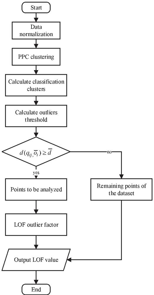
Figure 1 PPCLOF algorithm flow.
In PPCLOF algorithm, the dataset is preprocessed before LOF inspection. PPC clustering process is performed on the preprocessed dataset at first. In the clustering stage, for the objects in each category, the high-dimensional data objects are projected clustering. The projection index function is established. Then the relevant optimization algorithm is applied to solve the multi-dimensional projection index. So we obtain the optimal projection vector and correlation coefficient. For those objects whose distance from the center of the distance class is less than or equal to the radius, they are preliminarily judged as non-outliers. In fact, the main purpose of the clustering process is to prune non-outliers and obtain candidate sets of outliers. It would reduce unnecessary calculations in the LOF check process. The LOF process could be quickly implemented. Therefore, the time complexity of the PPCLOF algorithm would be lower. At the same time, because the LOF process is performed on the candidate set after pruning, the problem of wasting space resources is avoided.
After the high-dimensional data is reduced in dimensionality, the second stage is to calculate the data outlier factor. Call LOF method for the candidate dataset obtained in the first stage. Calculate the outlier factor LOF value of each data object. Then sort the obtained LOF values, and judge the first m points with the largest LOF values as outliers. The specific process is shown in Figure 1:
Since the PPCLOF algorithm has two stages, its time complexity consists of two parts. The stage of PCC process for marking the candidate set of outliers; the calculation of the LOF value for all candidate points, and the time required to sort the LOF values at the same time. The time complexity of the clustering algorithm is O(knt), where k is the number of classifications, t is the number of iterations during clustering, and n is the number of objects in the dataset. Usually and . The time complexity of the LOF method is O(N), where N is the number of data points in the outlier candidate set. Therefore, the time complexity T of PPCLOF is: . Normally, in a dataset, the number of outliers is far less than the number of normal points. So N generally does not exceed half of n. Assuming , the time complexity of the PPCLOF algorithm is about , because and . So we have . The time complexity of PPCLOF is .
3 Experiments Result and Discussion
3.1 Experiments on Real-world Data
Since there is currently no recognized outlier detection dataset, machine learning datasets are generally used to be outlier detection dataset. Control the number of outliers to about 5% of the total data. In order to verify the effectiveness of this method for detecting outliers in high-dimensional data, this paper uses the Lymphography dataset in the UCI public dataset [22] to conduct an experimental analysis of the PPCLOF algorithm and compare it with the existing outlier detection methods. The composition of the dataset is shown in Table 1.
Table 1 Lymphography dataset
| Number of Instances | 148 |
| Number of Attributes | 18 |
| Missing Values? | No |
| Number of Outliers | 6 |
| Classes | normal find, metastases, malign lymph, fibrosis |
The Lymphography dataset contains 148 instances, and each instance has 18 attributes. The dataset has 4 types of labels: normal find, metastases, malign lymph, and fibrosis. The least number of instances of the two types (normal find and fibrosis) account for 4.05% of the dataset, so these two types of sample points are regarded as outliers, the other 2 types of instances are regarded as normal sample points.
Outlier detection can be regarded as a two-classification problem, and the dataset is divided into two categories: abnormal value and normal value. Then the sample can be divided into true positive (TP), false positive (FP), true negative (TN) and false negative (FN). From this, a formula to evaluate the accuracy of the outlier detection method can be obtained:
True positive rate (TPR) represents the proportion of instances predicted to be positive and actually positive. False positive rate (FPR) represents the proportion of instances predicted to be positive and actually negative to all instances of negative class. The effect of the classifier is reflected by the distance between the classifier and the ideal classifier in the ROC graph, which is called EUC. The smaller the distance, the better the classification effect can be achieved. So it is used to indicate the detection accuracy of the outlier detection method.
The contrast method used in the experiment are ODC (Outlier Detection based Clusering) [23] and FindCBLOF (Find Cluster-Based Local Outlier Factor) [24]. They are outlier detection methods based on improved clustering algorithms and also contain two stages. This paper compares the three methods on Lymphography dataset, and the results are shown in Table 2. The accuracy of ODC, FindCBLOF and PCCLOF are 66.22%, 63.51% and 80.4%. The EUC of them are 0.8, 0.88 and 0.76. It can be seen that the precision of PPCLOF is relatively high.
Table 2 Test results of two approaches
| he | TP | FP | TN | FN | ACC | EUC |
| ODC | 6 | 22 | 92 | 28 | 66.22% | 0.8 |
| FindCBLOF | 6 | 24 | 68 | 40 | 63.51% | 0.88 |
| PPCLOF | 6 | 10 | 113 | 19 | 80.4% | 0.76 |
3.2 Experiments on Artificial Data
In order to verify the effectiveness of the model, this paper uses a Gaussian mixture model to generate multiple normal uncertain datasets containing different clusters. At the same time, another 100 special uncertain data points are generated in each artificial dataset. The method of generation is to independently generate uniformly random data points in the entire data space of each dataset. Because the generation mechanism of these 100 points is different from the generation mechanism of the three main clusters in each dataset, these 100 points can be considered as outliers in terms of the definition of outliers. In order to better evaluate the performance of the algorithm, this chapter artificially generated different datasets with 10 dimensions, the sizes were 1K, 5K, 100K, 200K and 1000K.
Figure 2 shows the ROC curve change on the artificial dataset. It can be clearly seen from the figure that the algorithm has obvious performance advantages. Especially when the false positive rate is relatively low, the algorithm in this paper can guarantee a true rate more than 70%, and its true positive rate is greater than ODC algorithm.
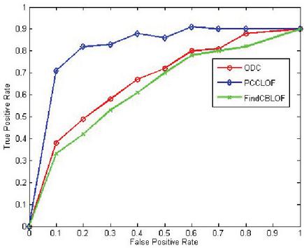
Figure 2 ROC diagram of dataset.
It can be observed from the figure that when the false positive rate of the algorithm is relatively high, the positive rate is also relatively high. When the false positive rate is relatively low, the algorithm has a relatively large advantage. However, the PPCLOF algorithm cannot guarantee a 100% detection rate. For example, when the false positive rate is 0.1, the correctness rate of the algorithm in this paper is always at the level of 0.72–0.73. It can be seen that the algorithm proposed by this paper still has lots of space for optimization. One of the reasons is the existence of nonlinearly correlated subspaces.
The previous analysis of the accuracy performance of the algorithm proved that the algorithm was better than other algorithm in accuracy. Also compare with the time results of the ODC algorithm. The time performance comparison result is shown in Figure 3:
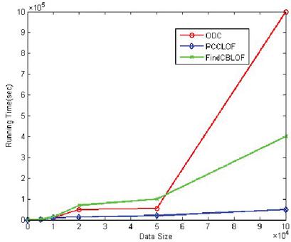
Figure 3 Time performance comparison.
As shown in the figure above, when the dataset is relatively small, the running time of PPCLOF and ODC is almost the same. Only when the dataset is relatively large, PPCLOF method shows obvious time efficiency advantages. It shows that if the dataset is large, the matrix calculation in the algorithm will bring a relatively large time load. The algorithm proposed does not require all data points involved in the calculation. Only a part of the sample points which selected by the cluster using radius as the threshold are need. In this way, it not only ensures the calculated results not have great deviations, but also improve time efficiency.
4 Conclusion
The PPCLOF method proposed in this paper first reduces the dimensionality of high-dimensional data to calculate the projection vector and correlation coefficient of the dataset, and get the result of data clustering. A small scale of category datasets are initially selected, then the outliers are calculated and determined by the LOF algorithm. According to the weaknesses of the LOF algorithm, the low-dimensional data is effectively cut to raise the efficiency and accuracy of the algorithm. So the algorithm does not require all data points to participate in the calculation. There are advantages in time and accuracy.
Acknowledgement
This work is supported by 2019 Chongqing Higher Education Teaching Reform Research Project: Research on the Reform of Cultivating Talents in Application-oriented Computing Disciplinary (Project No. 193356).
References
[1] Agovic Amrudin, Banerjee Arindam, Ganguly Auroop, Pro-topopescu Vladimir, ‘Anomaly detection using manifold embedding and its applications in transportation corridors’, Intelligent Data Analysis, vol. 13, no. 3, pp. 435–455, 2009.
[2] Mejia A F, Nebel M B, Eloyan A, et al., ‘PCA leverage: outlier detection for high-dimensional functional magnetic resonance imaging data’, Biostatistics, vol. 18, no. 3, pp. 521–536, 2017.
[3] Ju F, Sun Y, Gao J, et al., ‘Image outlier detection and feature extraction via L1-norm-based 2D probabilistic PCA’, IEEE Transactions on Image Processing, vol. 24, no. 12, pp. 4834–4846, 2015.
[4] MLA Sheri, Ahmad Muqeem, et al, ‘Background Subtraction using Gaussian-Bernoulli Restricted Boltzmann Machine’, IET Image Processing, vol. 12, no. 9, 2018.
[5] Lin, J., B. Wu, and W. Chen, ‘Adaptive Detection and Preprocessing Method for Abnormal Wind Speed of Wind Farm Based on Deep Boltzmann Machine’, Electrotechnical Society, pp. 205–212, 2018.
[6] Shenglian L, ‘Research of Distance-based Outliers Detection’, Computer Engineering and Applications, vol. 40, no. 33, pp. 73–75,94, 2004.
[7] Chunsheng Li, Shu Yu, Xiaogang Liu, ‘Research on outlier detection algorithm based on improved distance sum’, Computer Technology and Development, vol. 29, no. 3, pp. 97–100, 2019.
[8] Shou Zhaoyu, et al., ‘Outlier detection with enhanced angle-based outlier factor in high-dimensional data stream’, International Journal of Innovative Computing Information and Control, vol. 14, no. 5, pp. 1633–1651, 2018.
[9] Rehage, et al., ‘An angle-based multivariate functional pseudo-depth for shape outlier detection’, Journal of Multivariate Analysis: An International Journal, pp. 325–340, 2016.
[10] Tran L, Fan L, Shahabi C, ‘Distance-based outlier detection in data streams’, Proceedings of the Vldb Endowment, vol. 9, no. 12, pp. 1089–1100, 2016.
[11] Shaikh, Salman Ahmed, and H. Kitagawa, ‘Top-k Outlier Detection from Uncertain Data’, International Journal of Automation & Computing, vol. 11, no. 2, pp. 128–142, 2014.
[12] Liang Shaoyi, Han Deqiang, ‘Outlier detection based on neighborhood chain’, Countrol and Decision, vol. 34, no. 7, pp. 1433–1440, 2019.
[13] Henrion, Marc, et al., ‘CASOS: a subspace method for anomaly detection in high dimensional astronomical databases’, Statistical Analysis & Data Mining the Asa Data Science Journal, vol. 6, no. 1, pp. 53–72, 2013.
[14] Shao J, Wang X, Yang Q, et al., ‘Synchronization-based scalable subspace clustering of high-dimensional data’, Knowledge and Information Systems, vol. 52, no. 1, pp. 83–111, 2017.
[15] Ma, H., Y. Hu, and H. Shi, ‘Fault Detection and Identification Based on the Neighborhood Standardized Local Outlier Factor Method’, Industrial & Engineering Chemistry Research, vol. 52, no. 6, pp. 2389–2402, 2013.
[16] Friedman JH, Tukey JW, ‘A projection pursuit algorithm for exploratory data analysis’, IEEE Transactions on computers, vol. 100, no. 9, pp. 881–890, 1974.
[17] Ni Changjian, Cui Peng, ‘Projection pursuit dynamic clustering model’, Journal of Systems Engineering, vol. 22, no. 6, pp. 634–638, 2007.
[18] Xiong Pin, Lou Wengao, ‘Determination and analysis of reasonable values of key parameters in projection pursuit modeling’, Computer Engineering and Applications, vol. 52, no. 9, pp. 50–55, 2016.
[19] Lou Wengao, Qiao Long, ‘New exploration and empirical research on projection pursuit classification modeling theory’, Mathematical Statistics and Management, vol. 34, no. 1, pp. 47–58, 2015.
[20] Wang Jiayang, Li Zuoyong, ‘Projection pursuit of taboo search optimization and its application in water resources evaluation’, Journal of Chengdu University of Information Technology, pp. 715–718, 2006.
[21] M. M. Breunig, H. P. Kriegel, R. T. Ng, J. Sander, ‘LOF: Identifying Density-based Local Outliers’, SIGMOD, 2000.
[22] Igor Kononenko, Bojan Cestnik. ‘UCI Machine Learning Repository,’ Available: http://archive.ics.uci.edu/ml/datasets/Lymphography.
[23] Ahmed, Mohiuddin, and A. Naser, ‘A novel approach for outlier detection and clustering improvement’, Industrial Electronics & Applications IEEE, 2013.
[24] Jiang S., Li Q., ‘Clustering-Based Outlier Detection Method’, Fifth International Conference on Fuzzy Systems and Knowledge Discovery, pp. 429–433, 2008.
Biographies

Chen Chen is a PH.D. student at the Army Logistics University of PLA since autumn 2017. She attended the Chongqing University, majoring in Software Engineering where she received her B.Sc. in 2014. Chen then went on to purchase an M.SC. in Computer Science and Technology from Logistical Engineering University, Chongqing, China, in 2017. Chen is now mainly focusing on logistics informatization, information management and information system.

Kaiwen Luo is a Associate professor of the Army Logistic University, Chongqing, China. He received Ph.D. degree in Logistics informatization from Logistical Engineering University, Chongqing, China in 2016. His research focuses on logistics informatization and intelligent logistics equipment.

Lan Min is a professor of Chengdu University of Technology, Chengdu, China. Her research focuses on Mathematics and Applied Mathematics (Advanced Mathematics Education and Research).

Shenglin Li received his B.Sc. degrees in Mathematics and M.Sc. degrees in Computer Science and Technology from Southwest China Normal University, Chongqing. And Ph.D. degree in Logistics Informatization from Logistical Engineering University, Chongqing, China. He is a professor of Southwest University. His research focuses on Intelligent Science and Technology, Data Science and Big data Technology.
Journal of Web Engineering, Vol. 20_3, 743–758.
doi: 10.13052/jwe1540-9589.2038
© 2021 River Publishers