Optimal Design of Electrical Capacitance Tomography Sensor and Improved ART Image Reconstruction Algorithm Based On the Internet of Things

Feng Chen^*, Deyun Chen, Lili Wang and Botao Yang

School of Computer Science and Technology, Harbin University of Science and Technology, Harbin, China

E-mail: chenfeng@hrbust.edu.cn

*Corresponding Author

Received 25 March 2021; Accepted 25 April 2021; Publication 24 June 2021

Abstract

For the problems of low sensitivity, weak signal of high and low frequency and low signal-to-noise ratio in ECT, the mathematical model of the sensor is established. From the aspects of electrostatic field distribution and soft field effect, the influence of the structural parameters of the sensor on the sensor performance is analyzed. According to the influence of the components of the sensor on the sensitivity, the principle of optimal design is put forward. Based on the optimized Landweber image reconstruction algorithm, an ART image reconstruction algorithm with iterative correction is proposed, and the mathematical model of the algorithm is designed. According to constructing the target functional regularization term in the negative problems of electrical capacitance tomography, the iterative process of the modified art algorithm is deduced, and with adaptive step size, the convergence is speeded and accuracy of image reconstruction is improved. The experimental results show that the semi-convergence in the improved algorithm is obviously weakened, and the reconstructed image quality is better than that of the traditional art algorithm.

Keywords: Electrical capacitance tomography, optimal design of sensor, image reconstruction, modified ART iterative algorithm, convergence.

1 Introduction

Electrical Capacitance Tomography (ECT) is a process imaging technology based on the capacitive sensing principle developed in recent years. It is also a process parameter real-time online detection technology developed based on Computed Tomography (CT) technology [1, 2]. Belonging to one of Process Tomography (PT) technologies, it can visually measure closed pipelines or spaces and detect closed spaces by using externally applied alternating excitation electric fields. Conductive objects in the object field generate induced charges under the action of an applied electric field. Electric fields uniformly distributed outside closed pipelines or containers collect measured capacitance data from multiple angles, thus reconstructing the material distribution of conductive fluids in closed pipelines or spaces by using the measured data and sensitivity matrix. ECT technology has been applied in the fields of nondestructive testing, two-phase flow testing, combustion visualization and permafrost testing due to its advantages of non-radiation, non-invasion, low cost and availability of two-dimensional or three-dimensional process parameters. It is a process tomography technology with great development potential [3, 7].

The electrical capacitance tomography system consists of capacitance sensors, a data acquisition device and a reconstruction computer. The typical ECT system structure is shown in Figure 1.

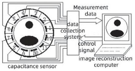
Figure 1 ECT system structure diagram.

Capacitance sensor is an important component of ECT system, which is mainly composed of detection electrode, radial shielding electrode, insulated pipeline and shielding cover [8]. It has great influence on the sensor’s sensitive field, data acquisition and reconstructed image quality [9]. The structure is shown in Figure 2.

Figure 2 Sensor structure diagram.

ECT technology aims at obtaining the dielectric constant distribution of different conductive substances and needs to solve both positive and negative problems. The positive problems is to solve the dielectric constant distribution and sensitivity matrix of the measured object field, while the negative problems is to solve the material distribution image according to the known dielectric constant distribution and sensitivity matrix of the measured object field. The key of ECT positive problems is the accuracy of sensor acquisition. It is necessary to solve the problems of low sensor sensitivity, weak detection signal and low signal-to-noise ratio, which are all related to the physical size of the sensor. However, the performance of the sensor is not only determined by the effective area of the measuring electrode. Although the effective area of the sensor can be increased by physical methods, a single increase in the effective area will produce noise interference, whereas a decrease in the effective area will reduce the sensitivity of the sensor acquisition. Therefore, the optimal design of the sensor should be comprehensively analyzed. ECT negative problems belongs to the first kind of Fredholm integral equation problem. Its solution is ill-posed and ill-conditioned, which makes it one of the main factors restricting ECT development. Therefore, how to solve the negative problems quickly and efficiently has received more and more attention. At present, the iterative algorithm is an effective method to overcome the problem in ECT negative problems. However, in the reconstruction process, the parameter selection is complex, often based on experience, and has great limitations [10, 12].

As people continue to explore the field of ECT technology, the technology has developed rapidly. In order to meet the needs of industrial development, more experts and scholars have joined the research of sensor design optimization and image reconstruction algorithms. In 2014, Q. Marashdeh et al. proposed a combination of several independent small plates to form a combined plate. The design of adaptive electrical capacitance tomography sensor. This scheme changes the sensitive field distribution by changing the voltage distribution on the combined plate, and further improves the image reconstruction quality [13]. In 2015, Z. Zeeshan et al. proposed that the AECVT sensor’s sensitive field calculation method based on the actual induced charge distribution is different from the traditional sensitive field calculation method based on boundary conditions. This method considers the interaction between electrodes [14]. In the field of image reconstruction, in 1997, the neural network algorithm was applied to the experiment of detecting multiphase flow. Nooralahiyan et al. used simulation experiments to demonstrate the feasibility of the method under experimental conditions [15]. In 2003, Warsito and others of Ohio State University in the United States conducted further research on neural networks and applied the multi-judgment optimal image reconstruction technology (NN-MOIRT) of dynamic neural networks to the electrical capacitance tomography system, and the images obtained were accurate Degree higher [16].

In this paper, aiming at the problem of sensor acquisition accuracy in ECT positive problems, 12-electrode UMIST ECT sensor was selected as the research object, and the influence of sensor design structural parameters on data acquisition was analyzed by improving the design of sensor physical model. At the same time, taking oil-water two-phase flow as measured fluid, the influence of sensor design structure on sensitivity under different distributions was analyzed. In the aspect of ECT negative problems, based on analyzing the characteristics of various image reconstruction algorithms, aiming at the problems of ART algorithm such as many iterations, slow convergence speed, smooth effect on media interface and difficulty in selecting iteration step size, etc., the optimized Landweber image reconstruction algorithm was also compared and analyzed, and ART image reconstruction algorithm based on regularization iterative correction was proposed, and the iteration formula for optimizing ART algorithm was deduced. The regularization term was added to the target function of the algorithm, and the method of adaptive weight coefficient was adopted in the meantime to improve the convergence speed. While ensuring the timeliness of image reconstruction, the reconstruction quality of the algorithm was significantly improved. The experimental results showed that the semi-convergence of the improved ART algorithm was significantly weakened, also the reconstructed image’s accuracy and speed were better than that of the traditional ART algorithm.

2 Theoretical Basis of Inductor Design

2.1 ECT System Mathematical Model

The ECT positive problems is to know the internal dielectric constant distribution and solve the boundary measurement capacitance value and sensitivity matrix of the sensor detection electrodes. Based on the electromagnetic field theory, the electromagnetic field in the capacitive sensor can be considered as a stable electrostatic field, which means there is no free charge in the field. Therefore, the point distribution in the sensor satisfies Laplace equation of the electrostatic field, as shown in formula (1).

$$\nabla \cdot [{\epsilon }_0\epsilon (x,y)\nabla \varphi (x,y)]=0$$

(1)

In the formula: $\epsilon (x,y)$ and $\varphi (x,y)$ are the dielectric constant distribution function and potential distribution function respectively, and are the divergence operator and gradient operator respectively. When electrode i is the source electrode (excitation electrode), its corresponding boundary condition can be expressed as follows:

$${\varphi }^{(i)}=\{\begin{array}{c}V(x,y)\subseteq {\mathrm{\Gamma }}_i\hfill \\ 0(x,y)\subseteq {\mathrm{\Gamma }}_k+{\mathrm{\Gamma }}_s+{\mathrm{\Gamma }}_g\hfill \end{array}$$

(2)

In the formula: ${\mathrm{\Gamma }}_i,{\mathrm{\Gamma }}_s,{\mathrm{\Gamma }}_g$ are the positions of electrode $i(i=1,2,3\mathrm{\dots },12)$, shielding layer and radial electrode respectively. The electric field strength can be expressed as:

$E(x,y)=-\nabla \varphi (x,y)$

(3)

When the electrode i is the excitation electrode and the electrode j is the detection electrode, the induced charge on the electrode j obtained by Gaussian theorem is:

$$Q_{i,j}={\oint }_{{\mathrm{\Gamma }}_j}{\epsilon }_0\epsilon (x,y)E\widehat{n}\mathit{d}l=-{\oint }_{{\mathrm{\Gamma }}_j}{\epsilon }_0\epsilon (x,y)\nabla \varphi (x,y)\cdot \widehat{n}\mathit{d}l$$

(4)

In the formula, ${\mathrm{\Gamma }}_j$ is a closed curve surrounding the electrode j, and n is the unit normal vector of the curve.

When $Q_{i,j}$ is determined, the capacitance $C_{i,j}$ between electrode i and electrode j is:

$$C_{i,j}=\frac{Q_{i,j}}{U_{i,j}}$$

(5)

In the formula $U_{i,j}$ is the voltage between electrode i and electrode j.

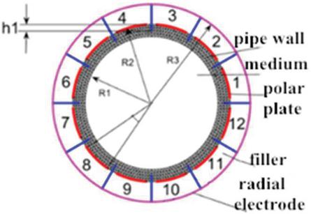
Figure 3 Cross-sectional view of ECT sensor.

2.2 Sensor Optimization Design

When designing the simulation of the sensor, the electromagnetic field characteristics of the measured object field need to be modeled first. In ECT system, the propagation speed of the electromagnetic wave in the vacuum is much faster than that of the measured object, so the electromagnetic field in ECT sensor can be regarded as an approximately stable electrostatic field [17]. Based on this theory, sensor simulation can be described and solved by electrostatic field theory. Therefore, the ECT sensor can be idealized: the detection process is a static experiment process. The capacitor plate and the shielding cover are infinitely extended along the axial direction of the pipeline. Ignore the edge effect of the polar plate. The dielectric constant of the measured current type is not affected by the applied voltage.

Firstly, through modeling, a sensor sensitive array electrode model with a single layer of 12 electrodes is built and a single-electrode excitation mode is adopted. The mode can be described as follows: electrode C${}_{\mathrm{1}}$ applies excitation to measure the charge amount on a total of 11 electrodes C${}_{\mathrm{2}}$–C${}_{\mathrm{12}}$. Then, excitation is sequentially applied to the remaining electrodes until electrode C${}_{\mathrm{11}}$ is excited, in the next, measure the charge amount on electrode C${}_{\mathrm{12}}$. According to the formula $M=N(N-1)/2$, where n represents the number of sensor electrodes and m represents the number of acquisition capacitance values, a total of 66 capacitance values can be obtained. The cross-sectional view of the sensor is shown in Figure 3.

Secondly, analyze and solve the sensor by a finite element method. First of all, assuming that the edge effect of the electrode along the axial direction is negligible. When calculating the electric field, it is considered that the electrodes and shielding layer are infinitely long, the distribution of multiphase medium along the axial direction is unchanged, and there is no free charge on the pipeline interface. Based on the above assumption, the boundary problem with the solution is as follows:

$$\{\begin{array}{cc}\nabla \cdot [\epsilon (x,y)\nabla u(x,y)]=0\mathit{\hspace{1em}}\hfill & \\ {u(x,y)|}_{(x,y)\in R_i}=U\mathit{\hspace{1em}}\hfill & (i=1,2,\mathrm{\dots },12)\hfill \\ {u(x,y)|}_{(x,y)\in R_k+R_s+R_g}=0\mathit{\hspace{1em}}\hfill & (k=1,2,\mathrm{\dots }12k\ne i)\hfill \end{array}$$

(6)

In the formula: $\epsilon$ is the medium distribution in the pipeline; $u$ is potential distribution; $U$ is the voltage applied to the electrode. $R_i$, $R_s$ and $R_g$ are electric charge on the electrode, the shielding cover and the radial electrode respectively. Assuming that the voltage applied to the excitation electrode is $U$ and the detection electrode, radial electrode and shielding electrode are grounded, the charge on the polar plate $k$ can be calculated as follows:

$$Q_k={\int }_{S_k}\epsilon (x,y)\frac{\partial u}{\partial n}\mathit{d}S$$

(7)

In the formula $S_k$ is the $k$-th electrode.

To analyze the influence of sensor structure parameters on measurement accuracy, firstly, the parameters of the sensor without radial electrode are defined: the electrode plate adhered to the pipe wall has the same length, width H $=$ 8 mm, electrode plate opening angle $\theta ={10}^{\circ }$, pipe inner radius R1 $=$ 66.8 mm, pipe thickness 5mm, shielding layer thickness 5 mm, pipe wall relative dielectric constant ${\epsilon }_1=5.8$, shielding layer relative dielectric constant ${\epsilon }_2=2.2$. Hollow tube dielectric constant ${\epsilon }_w=81$, full tube dielectric constant ${\epsilon }_o=8$. ${\epsilon }_w$ and ${\epsilon }_o$ represent the state of all water and all oil respectively. Among them:

${\epsilon }_w$	$=78.54[1-4.579\times 10-3(T-25)+1.19\times 10-5{(T-25)}^2$
	$\mathrm{\hspace{1em}}-2.8\times 10-8{(T-25)}^3]$	(8)

T is the temperature, unit ${}^{\circ }$C, due to the cooling treatment of the measuring pipeline. The preset temperature range from $-5^{\circ }$C to 25${}^{\circ }$C, the dielectric constant of water changes between 90.6 and 78.5. The dielectric constant of petroleum is a non-single value function, and the composition of petroleum is complex, usually between 2 and 10. To analyze the sensor performance linearly, the experiment is idealized in this paper: the internal temperature of the pipeline is constant during the measurement, the dielectric constant of water in the pipeline is 81, and the dielectric constant of oil is 2.2. Then, by changing the structural parameters of the sensor, the influence brought by the change of different parameter values is analyzed. The sectional view of the sensor without radial electrodes is shown in Figure 4.

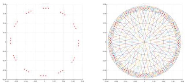
Figure 4 Sectional view of sensor without radial electrode.

To analyze the influence of the presence of radial electrode on the sensor design, set the relevant parameters of the radial electrode sensor: the relevant dielectric constants $\epsilon$1, $\epsilon$2, $\epsilon$3, $\epsilon$4 are the same, i.e. the insulating material, pipe wall filler and measuring substance are unchanged. In the initial state, the width of the radial shielding electrode is F $=$ 5 mm, the depth of the inserted polar plate is h1 $=$ 1.5 mm, and its outer edge is tightly attached to the shielding cover. A sectional view of that sensor with the radial electrode is shown in Figure 5.

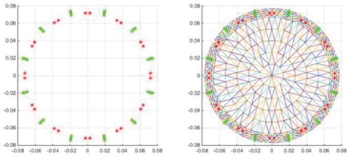
Figure 5 Sectional view of a radial electrode sensor.

Firstly, under the circumstances that other parameters unchanged, analyze the influence of the radial electrode on the sensor. The radial electrode can control the power line inside the polar plate and block the power line between the adjacent substrates so that the electric field mainly acts on the medium inside the pipeline and has an enhanced effect on the sensitive field. To analyze more accurately, the sensitive field numerical distribution of adjacent plates, 3 plates at intervals and 5 plates at intervals is selected for analysis.

Table 1 Distribution of sensitive fields

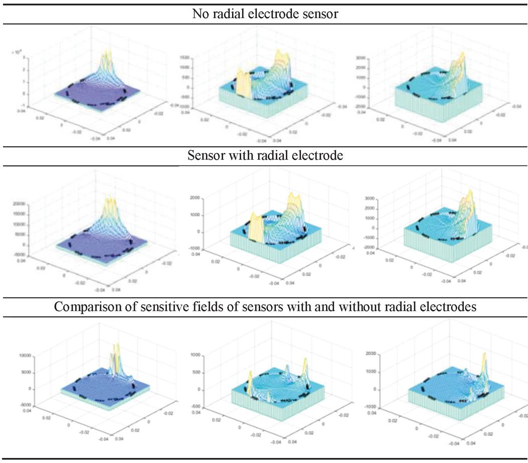Based on the analysis in Table 1, the distribution of the sensitive field is unimodal, and the amplitude of the sensitive field is higher as it gets closer to the excitation plate, whereas the amplitude is lower as it gets further away from the excitation plate, and the sensitive field area of the receiving electrode decreases more obviously as it gets further away. This shows that in the single excitation mode, the further away from the excitation plate, the lower the accuracy of the collected values of the receiving plate during measurement. The main reason for this phenomenon is the influence of excitation mode, excitation voltage and the level of the sensitive field in the center of the pipeline. With the installation of radial electrode inside the sensor, the sensitive field near the excitation electrode is enhanced, and the sensitive field of the receiving electrode is also enhanced compared with the non-radial electrode mode. The analysis shows that the radial electrode can reduce the measurement error caused by the electric field effect, effectively increase the measurement accuracy of the sensitive field and improve the sensitivity of the sensor. At the same time, analysis shows that the non-linear problem of ECT sensor will distort image reconstruction, i.e. “soft field” effect, which is also one of the obvious differences between electric signal measurement and ray signal measurement [18, 19].

Secondly, the influence on the sensor performance is analyzed by changing the opening angle of the polar plate $\theta$, the width w of the measuring polar plate, the depth h1 and the width F of the radial electrode, and the difference of the empty/full tube capacitance is used as an index to measure the sensor measurement performance. The larger the difference between the empty/full tube capacitance, the better the sensor performance, $C_{i,j}$ indicates that when the i-th excitation electrode acts, the capacitance value data on the j-th reception electrode is marked with 1-12 polar plates in the counterclockwise direction as shown in Figure 3, with the excitation electrode as 1 polar plate and the others as reception polar plates. Empty/full tube capacitance values are different with different angles between the sensors, which is shown in Tables 2 and 3.

Table 2 Change of empty pipe capacitance value of sensor with changing plate opening angle (Unit/pF)

Electrode Pair	$\theta =5^{\circ }$	$\theta ={10}^{\circ }$	$\theta ={20}^{\circ }$	$\theta ={25}^{\circ }$
$C_{1,2}$	0.0319	0.0738	0.2461	0.3236
$C_{1,3}$	0.0090	0.0197	0.0546	0.0666
$C_{1,4}$	0.0046	0.0101	0.0273	0.0331
$C_{1,5}$	0.0031	0.0068	0.0182	0.0220
$C_{1,6}$	0.0025	0.0055	0.0146	0.0177

Table 3 Change of full tube capacitance value of sensor with changing plate opening angle (Unit/pF)

Electrode Pair	$\theta =5^{\circ }$	$\theta ={10}^{\circ }$	$\theta ={20}^{\circ }$	$\theta ={25}^{\circ }$
$C_{1,2}$	0.0452	0.1191	0.4448	0.5729
$C_{1,3}$	0.0265	0.0669	0.2259	0.2829
$C_{1,4}$	0.0193	0.0478	0.1535	0.1901
$C_{1,5}$	0.0159	0.0387	0.1207	0.1485
$C_{1,6}$	0.0142	0.0344	0.1055	0.1294

Table 4 Change of capacitance difference between empty and full tubes of sensor with changing plate opening angle (Unit/pF)

Electrode Pair	$\theta =5^{\circ }$	$\theta ={10}^{\circ }$	$\theta ={20}^{\circ }$	$\theta ={25}^{\circ }$
$C_{1,2}$	0.0133	0.0453	0.1988	0.2493
$C_{1,3}$	0.0175	0.0472	0.1714	0.2162
$C_{1,4}$	0.0147	0.0377	0.1263	0.1571
$C_{1,5}$	0.0127	0.0319	0.1025	0.1265
$C_{1,6}$	0.0117	0.0289	0.0909	0.1117

Based on the data analysis in Table 4, on the occasion that the length of the measuring polar plate is constant, the effective area of the measuring polar plate increases with the increase of the polar plate opening angle, and the sensitivity of the sensitive field also increases. However, if the polar plate opening angle is too large, under the condition that the length and number of polar plates are unchanged, the sensitivity between adjacent polar plates will increase, the sensitivity of measuring polar plates acting on the inner core area of the pipeline will decrease, while the measurement error for core flow will increase. In consequence, the selection of the polar plate opening angle should be analyzed comprehensively.

Empty/full tube capacitance values are different with different electrode insertion depth, which is shown in Tables 5 and 6.

Table 5 Changes in capacitance value of sensor empty pipe (Unit/pF) when radial electrode depth is changed

Electrode Pair	$h_1=0$ mm	$h_1=1.5$ mm	$h_1=3$ mm	$h_1=4.5$ mm
$C_{1,2}$	0.1780	0.2223	0.1227	0.0495
$C_{1,3}$	0.0440	0.0510	0.0310	0.0155
$C_{1,4}$	0.0223	0.0256	0.0157	0.0080
$C_{1,5}$	0.0149	0.0172	0.0105	0.0054
$C_{1,6}$	0.0120	0.0138	0.0085	0.0043

Table 6 Changes in capacitance value of sensor full tube (Unit/pF) when radial electrode depth is changed

Electrode Pair	$h_1=0$ mm	$h_1=1.5$ mm	$h_1=3$ mm	$h_1=4.5$ mm
$C_{1,2}$	0.2711	0.3491	0.2149	0.0250
$C_{1,3}$	0.1139	0.1941	0.1165	0.0090
$C_{1,4}$	0.1156	0.1389	0.0815	0.0049
$C_{1,5}$	0.0952	0.1128	0.0652	0.0034
$C_{1,6}$	0.0855	0.1004	0.0576	0.0027

Table 7 Variation of capacitance difference between empty and full tubes of sensor when radial electrode depth is changed

Electrode Pair	$h_1=0$ mm	$h_1=1.5$ mm	$h_1=3$ mm	$h_1=4.5$ mm
$C_{1,2}$	0.0930	0.1268	0.0922	-0.0245
$C_{1,3}$	0.1139	0.1431	0.0855	-0.0065
$C_{1,4}$	0.0934	0.1132	0.0658	-0.0031
$C_{1,5}$	0.0803	0.0956	0.0547	-0.0020
$C_{1,6}$	0.0734	0.0866	0.0491	-0.0016

According to the analysis of the data in Table 7, the radial electrode can effectively weaken the electric field effect and improve the measurement accuracy of the sensor. When the radial electrode increases with the insertion depth of the tube wall, the sensitivity of the sensor will increase. However, as the radial electrode goes deep into the tube wall, the radial electrode will react to the static electric field, reducing or even covering the electric field of the original measuring electrode. When the radial electrode passes through the plate, the effect of the electric field will react to the electric field of the plate, resulting in the coverage of the measurement data and serious distortion of the image. Therefore, when installing radial electrodes, the maximum effect can be achieved only by combining the width of the electrodes.

Empty/full tube capacitance values are different with different plate width, which is shown in Tables 8 and 9.

Table 8 Changes in capacitance value of sensor empty pipe (Unit/pF) when changing plate width

Electrode Pair	$\mathit{\text{H}}=10$ mm	$\mathit{\text{H}}=15$ mm	$\mathit{\text{H}}=20$ mm	$\mathit{\text{H}}=25$ mm
$C_{1,2}$	0.0841	0.0698	0.0562	0.0894
$C_{1,3}$	0.0229	0.0390	0.0373	0.0358
$C_{1,4}$	0.0117	0.0205	0.0199	0.0194
$C_{1,5}$	0.0079	0.0140	0.0138	0.0135
$C_{1,6}$	0.0064	0.0138	0.0113	0.0111

Table 9 Changes in capacitance value of sensor full tube (Unit/pF) when changing plate width

Electrode Pair	$\mathit{\text{H}}=10$ mm	$\mathit{\text{H}}=15$ mm	$\mathit{\text{H}}=20$ mm	$\mathit{\text{H}}=25$ mm
$C_{1,2}$	0.0974	0.1083	0.0948	0.1236
$C_{1,3}$	0.0612	0.1391	0.1301	0.0476
$C_{1,4}$	0.0470	0.0584	0.0482	0.0415
$C_{1,5}$	0.0399	0.0525	0.0441	0.0384
$C_{1,6}$	0.0364	0.0495	0.0420	0.0368

Table 10 Changes of capacitance difference between empty and full tubes of sensor when changing plate width (Unit/pF)

Electrode Pair	$\mathit{\text{H}}=10$ mm	$\mathit{\text{H}}=15$ mm	$\mathit{\text{H}}=20$ mm	$\mathit{\text{H}}=25$ mm
$C_{1,2}$	0.0133	0.0308	0.0386	0.0342
$C_{1,3}$	0.0384	0.0307	0.0189	0.0119
$C_{1,4}$	0.0352	0.0379	0.0283	0.0220
$C_{1,5}$	0.0320	0.0385	0.0303	0.0248
$C_{1,6}$	0.0300	0.0381	0.0308	0.0257

According to the data analysis in Table 10, the width of the measuring polar plate increases, the effective area of the polar plate expands. Under the condition of unchanged polar plate opening angle and radial electrode, the fluid flowing through the polar plate increases in unit time, the measuring time of the polar plate increases, and the signal changes slowly. Not sensitive to high-frequency signals in fluid. The width of the polar plate is short. Although the flowing time in unit time is shorter and the distinction between high and low-frequency signals is obvious, it also leads to the reduction of the effective measurement area of the sensor and the reduction of the measurement sensitivity.

According to the experimental analysis, when the sensor size is unchanged, when the sensor’s acquisition performance is the best, the sensor parameters are: plate opening angle $\theta ={25}^{\circ }$, radial electrode insertion depth $h_1=1.5$ mm, plate width $\mathit{\text{H}}=15$ mm.

The ECT system is mostly used for high-pressure fluid transportation detection, and the thickness of the pipe wall should be reasonably selected. If the pipe wall is too thin, the ability to withstand internal pressure is low and the mechanical strength is poor. If the pipe wall is too thick, the internal sensitivity will decrease due to the influence of the high sensitivity of the pipe wall. The filling material of the shield shall be a material with low dielectric constant, such as insulating thermal grease and other materials. On the one hand, radial electrodes and measuring plates can be fixed. On the other hand, the sensitivity of the internal sensor is increased while external electric field interference is effectively blocked.

3 Image Reconstruction

The non-iterative class is a fast imaging algorithm used earlier in ECT, but its imaging effect is general, suitable for online fast qualitative imaging, and cannot provide accurate quantitative information. The iterative algorithm is an effective method to overcome the ill-posedness of the negative problems of ECT, but its parameter selection is more complicated, and the selection is mostly based on experience, which has great limitations.

The ECT negative problems is to know the sensor measurement data and the distribution of the fluid in the pipeline, and to inverse the specific image, that is, the image reconstruction process. To compare the effect of each reconstruction algorithm in image reconstruction, LBP, TikHonov, Landweber and ART algorithms are selected for image reconstruction analysis. The LBP form is: $G=S^{T}C$. TikHonov takes the form of: $G={(S^{T}S+\alpha I)}^{-1}{S}^{T}C$. Landweber takes the form of $G_{k+1}=G_k-{\alpha }_k{S}^T(S{G}_k-C)$, three iterative algorithms, all of which are preset to iterate 1000 times. According to the above algorithm principle, image simulation reconstruction is carried out.

Table 11 Preset distributions and reconstruction algorithms

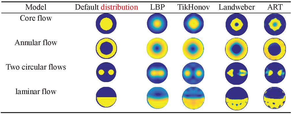According to the analysis in Table 11, when reconstructing the core flow, although regularization algorithm and LBP algorithm can obtain a clearer outline of the default model, in other distribution, the results of the reconstruction algorithm severely smeared sharp changes in the relative dielectric constant distribution, and the quality of the image formed is not high. ART algorithm and Landweber algorithm can get the outline of the default model clearly and have good imaging effect.

To evaluate the performance of various image reconstruction algorithms, It is measured by calculating the relative error (IE) and correlation coefficient (CC) of the reconstructed image, which are defined in Equations (9), (10).

$$IRE=\frac{\parallel \widehat{g}-g\parallel }{\parallel g\parallel }$$	(9)
$$CC=\frac{{\sum }_{i=1}^n(\widehat{g}-\widehat{\widehat{g}})\cdot (g-\widehat{g})}{\sqrt{{\sum }_{i=1}^n{(\widehat{g}-\widehat{\widehat{g}})}^2\cdot {(g-\widehat{g})}^2}}$$	(10)

In the formula: $g$ indicates the reconstruction result, represents the collection of pixels during image reconstruction; $\widehat{g}$ expressed as a preset dielectric constant; $\overline{g}$ represents the average value of reconstruction results; $\overline{\widehat{g}}$ indicates the average value of the preset dielectric constant.

Table 12 Error comparison of reconstructed images

Model	LBP	TikHonov	Landweber	ART
Core flow	0.53267	0.40019	0.43932	0.39617
Annular flow	0.86999	0.57386	0.47418	0.47163
Two circular flows	0.43628	0.38321	0.44627	0.51067
laminar flow	0.73094	0.50039	0.49922	0.45363

Table 13 Time comparison of reconstructed images (Unit/s)

Model	LBP	TikHonov	Landweber	ART
Model	LBP	TikHonov	Landweber	ART
Core flow	0.003229	2.560738	3.393293	6.334270
Annular flow	0.001786	2.512516	3.375166	7.125441
Two circular flows	0.001783	2.656619	3.480431	6.633416
laminar flow	0.001991	2.725233	3.431128	6.281759

According to the data analysis in Tables 12 and 13, in the four default models, using reconstruction quality and reconstruction time for analysis. In terms of imaging time, LBP imaging speed is the fastest while ART imaging speed is the slowest. In terms of reconstruction quality, the reconstruction quality of the iterative algorithm is higher than that of a non-iterative algorithm. On the imaging effect, the imaging effect of a single object is better than that of the multiple objects, which is caused by the nonlinearity of ECT sensitive field.

To better analyze the performance of Landweber and ART algorithms, under the same conditions, the reconstructed image error values obtained were compared and analyzed through 1,000 iterations respectively.

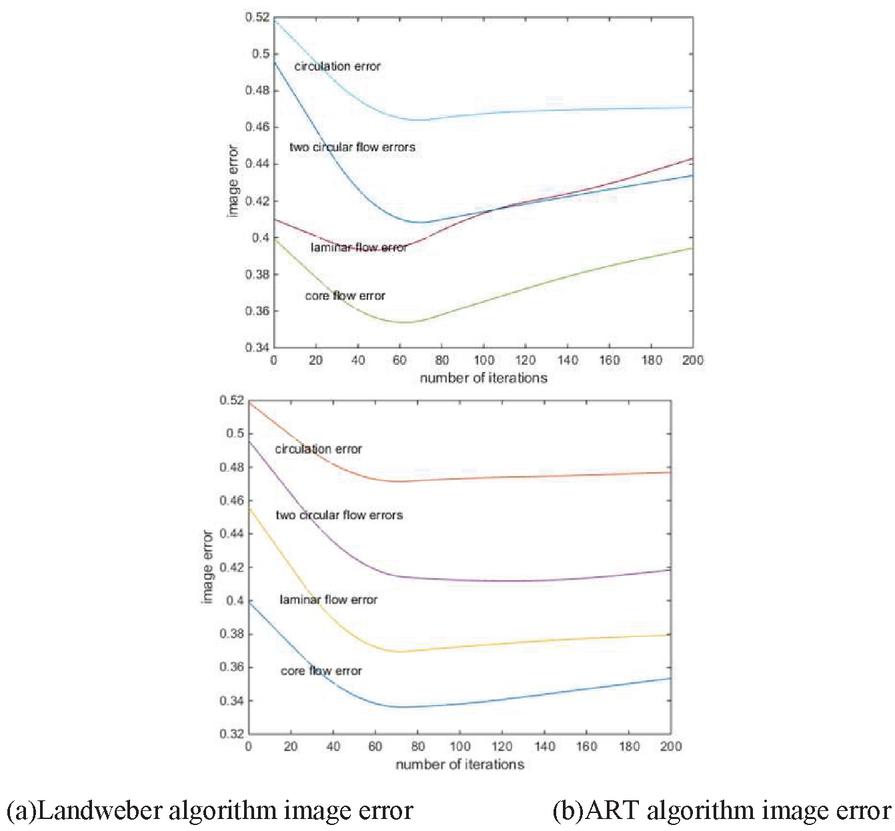
Figure 6 Image error comparison.

According to the analysis of Figure 6(a) and 6(b), Landweber algorithm needs many iterations to obtain the minimum value, resulting in slow convergence speed and semi-convergence. After the error reaches a minimum, the error increases with the number of iterations. For ART algorithm, the residual of projection value is used to carry out back-projection uniformly along the ray direction one by one, and the image is corrected continuously. That is, SOR algorithm is used to solve the standard minimum norm solution of linear equations until it meets the requirements, which can better avoid the semi-convergence phenomenon of nonlinear rebound. From the analysis of non-linear rebound of image error, ART algorithm has good adaptability to semi-convergence in the iterative process, and its error rebound is lower than Landweber algorithm while the number of iterations increases.

3.1 ART Algorithm Based on Electrical Capacitance Tomography

The basic idea of ART algorithm is to give any initial value of reconstruction area, and then uniformly back project the residual of projection value along the ray direction one by one, and continuously correct the image until it meets the requirements. Therefore, ART algorithm is also called iterative reconstruction algorithm with ray correction.

First, the pre-reconstructed continuous image $f(x,y)$ is divided into $N$ regions, and $f(x,y)$ in each region is regarded as pixels and is recorded as. In the next, based on the imaging physical process and the corresponding mathematical model, the linear equations between the reconstructed image and the projection data are established.

$\{\begin{array}{c}\hfill w_{11}{f}_1+w_{12}{f}_2+w_{13}{f}_3+\mathrm{\cdots }+w_{1N}{f}_N=p_1\hfill \\ \hfill w_{21}{f}_1+w_{22}{f}_1+w_{23}{f}_1\mathrm{\cdots }+w_{2N}{f}_N=p_2\hfill \\ \hfill \mathrm{\dots }\hfill \\ \hfill w_{M1}{f}_1+w_{M2}{f}_1+w_{M3}{f}_1\mathrm{\cdots }+w_{MN}{f}_N=p_M\hfill \end{array}$

(11)

In the formula: M is the total number of projection rays; $w_{ij}$ is a weight factor, it reflects the contribution of pixels $f_j$ to projection $p_i$. $p_i$ is the sum of rays of ray $i$. The task of ART image reconstruction is to calculate $f$ from $w,p$, and its specific steps are: presetting the initial value of the image. The initial value will affect the convergence rate (iteration number) and will not affect the final solution. Theoretically, the initial value should be selected according to prior knowledge, and it is customary to take the correction value of the image calculated according to the following formula:

$$f_j^{(k+1)}=f_j^{(k)}+\lambda \frac{p_i-\left({\sum }_{n=1}^N{f}_n^{(k)}{\omega }_{in}\right)}{{\sum }_{n=1}^N\omega _{ij}{}^2}{\omega }_{ij}$$

(12)

In the formula:kis the number of iterations; $1\le i\le M$; $1\le j\le M$. $\lambda$ is the relaxation factor $(0<\lambda <2)$. When all projection data are used, a complete iteration is completed. The image is corrected repeatedly until the convergence criterion is satisfied. Usually, only a limited number of iterations can be used, so convergence criteria must be selected. The common convergence criterion is to make $U^{(k)}={\sum }_{i=1}^N{(p_i-f^{(k)}{\omega }_i)}^2$ when ${(U^{(k)}N)}^{1/2}<e(0<e<1)$ to stop iteration at that time.

In the negative problems of electrical capacitance tomography, based on the linear model of dielectric constant to capacitance mapping, capacitance measurement value is usually discretized, linearized and normalized with sensitive field and substance distribution as shown in formula (13).

$$C=SG$$

(13)

Among them, $C$ is a capacitance measurement value; $S$ represents sensitive field; $G$ is the distribution of matter, $C\in R^I$, $G\in R^J$, $S\in R^{IXJ}$. Among them, $I$ is the measurable number of independent capacitors while $J$ is the number of pixels in the imaging region.

For each iteration of ART, only one projection data is used, and the iteration formula of ART algorithm is obtained by combining ART mathematical model formulas (11), (12) and ECT system model formula (14):

$$G_k=G_{k-1}+\frac{(C_k-S_k{G}_{k-1})}{{\parallel S_k\parallel }^2}S_k{}^T$$

(14)

Among them, $S_k$ represents the k-th row of the sensitivity matrix, the ART algorithm iteration is based on the k-th equation in Equation (10). In the k-th iteration, only the k-th normalized capacitance value is used to update the normalized dielectric constant distribution.

3.2 ART Algorithm Based on Regularization Iterative Correction

Iterative image reconstruction algorithms have always been a key research area. Because iterative image reconstruction algorithms are based on the least square criterion, they have common improvement forms. In 2018, Liu Xianglong and others proposed an optimized Landweber algorithm in electromagnetic tomography (EMT) [20]. This algorithm has become a new exploration of iterative algorithm optimization in EMT image reconstruction due to its advantages of flexible parameter selection, short reconstruction time and high reconstruction quality. The core idea of the algorithm is to first correct the target universal function of the inverse electromagnetic tomography problem and add a regularization term to it. Secondly, the method of adaptive weight coefficient is adopted to solve the optimal step size by v-acceleration method proposed by BrakHage et al. [21]. Based on the idea of this method, this paper proposes an ART algorithm based on regularization iterative correction. The core idea of this algorithm is as follows:

• TikHonov algorithm is used as the initial value of the reconstructed image.

• Revise the objective universal function and derive the optimized iterative formula of ART algorithm

$minf(G_k)$	$={\displaystyle \frac{1}{2}}\{{\alpha }_k\parallel G_k+{\displaystyle \frac{(C_{k+1}-S_{k+1}{G}_k)}{{\parallel S_{k+1}\parallel }^2}}S_{k+1}{}^T{\parallel }^2$
	$\mathrm{\hspace{1em}}+{\beta }_k\parallel G_k-G_{k-1}{\parallel }^2\}$	(15)

Among them, the first term is the difference between the calculated capacitance value and the actual capacitance value; The second term is the difference in capacitance sensitivity between the current moment and the previous moment, ${\alpha }_k,{\beta }_k$ are the weighting factors of the related terms respectively.

The derivative of $f(G_k$) with respect to $G_k$ is

$\nabla f(G_k)={\alpha }_k\left(G_k+{\displaystyle \frac{(C_{k+1}-S_{k+1}{G}_k)}{{\parallel S_{k+1}\parallel }^2}}S_{k+1}{}^T\right)+{\beta }_k(G_k-G_{k-1})$

(16)

Therefore, the iterative form is as follows:

$G_{k+1}$	$=G_k+\nabla f(G_k)=G_k+{\alpha }_k\left(G_k+{\displaystyle \frac{(C_{k+1}-S_{k+1}{G}_k)}{{\parallel S_{k+1}\parallel }^2}}S_{k+1}{}^T\right)$
	$\mathrm{\hspace{1em}}+{\beta }_k(G_k-G_{k-1})$	(17)

• v-acceleration method is used to solve the optimal value of ${\alpha }_k,{\beta }_k$. The core idea of v-acceleration method is to solve the problem iteratively in each step.

$$x_k^{\delta }=x_{k-1}^{\delta }+{\mu }_k(x_{k-1}^{\delta }-x_{k-2}^{\delta })+{\omega }_k{A}^{*}(y_{\delta }-A{x}_{k-1}^{\delta })$$

(18)

Among them, ${\mu }_0=0,{\omega }_0=(4v+2)/(4v+1)$, parameter v is generally selected according to experience. For $k\ge 1$, there are the following iterative methods:

$$\{\begin{array}{c}\hfill {\alpha }_k=4\frac{(match2k+2v+1)(k+v)}{(k+2v)(2k+4v+1)(2k+2v-1)}\hfill \\ \hfill {\beta }_k=\frac{k(2k-1)(2k+2v+1)}{(k+2v)(2k+4v+1)(2k+2v-1)}\hfill \end{array}$$

(19)

From Equations (13)–(18), the iterative formula of ART algorithm based on regularization iterative correction can be deduced as shown in Equation (20).

$$\{\begin{array}{c}\hfill G_{k+1}=P\left[G_k+{\alpha }_k\frac{(C_{k+1}-S_{k+1}{G}_k)}{{\parallel S_{k+1}\parallel }^2}S_{k+1}{}^T+{\beta }_k(G_k-G_{k-1})\right]\hfill \\ \hfill P[f(G)]=\{\begin{array}{cc}0\mathit{\hspace{1em}}\hfill & \mathit{if}(G)<0\hfill \\ f(G)\mathit{\hspace{1em}}\hfill & \mathit{if}\mathrm{\hspace{0.25em}0}\le f(G)\le 1\hfill \\ 1\mathit{\hspace{1em}}\hfill & \mathit{if}(G)>1\hfill \end{array}G\hfill \end{array}$$

(20)

Among them, $G_0$ is the capacitance value solved by TikHonov algorithm used as the initial value, and Equation (19) is used to solve ${\alpha }_k,{\beta }_k$. The V parameter takes 6 as the projection operator [22].

The optimized ART algorithm is compared with the algorithm in reference [20], and the Matlab simulation principle is applied to carry out image reconstruction under the same experimental conditions with 1,000 iterations as the termination condition and four default distributions as the research images.

Table 14 Comparison of images reconstructed by optimization algorithm

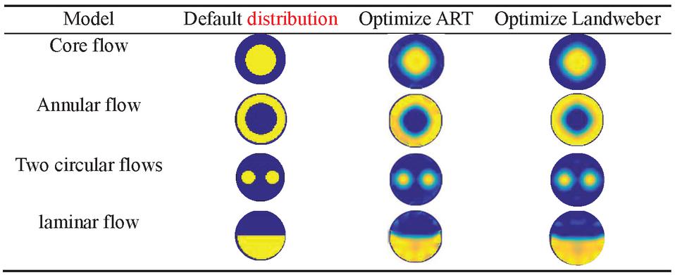Table 15 Comparison of reconstruction errors of optimization algorithms

Model	Optimize ART	Optimize Landweber
Core flow	0.2958	0.3125
Annular flow	0.3762	0.4140
Two circular flows	0.2731	0.2913
laminar flow	0.3264	0.3656

Table 16 Coefficient comparison of reconstructed images

Model	Optimize ART	Optimize Landweber
Core flow	0.7364	0.5543
Annular flow	0.7423	0.5434
Two circular flows	0.5242	0.3343
laminar flow	0.7432	0.6543

Table 17 Comparison of reconstruction time of optimization algorithms (Unit/s)

Model	Optimize ART	Optimize Landweber
Core flow	2.2200	2.0993
Annular flow	2.2711	2.1701
Two circular flows	2.2430	2.2161
laminar flow	2.2331	2.1458

According to the analysis of Tables 14–17, the optimized ART and Landweber algorithms can better overcome the imaging of multiple objects, and both can obtain a clearer restoration distribution. In terms of annular flow, the optimized Landweber algorithm still has a large edge effect problem inside the electric field. Although the optimized ART algorithm exacerbates the internal edge effect problem, it better restores the sensor boundary value distribution, Compared with the optimized Landweber algorithm, the image reconstruction error has been reduced by 0.0167, 0.0378, 0.0182, 0.0392, and the reconstruction correlation coefficient has increased by 0.1821, 0.1989, 0.1988, 0.0889 respectively. The two optimized algorithms have the same order of magnitude in reconstruction time. But the Landweber algorithm is slightly faster than the ART algorithm. The accuracy of the optimized ART algorithm on the reconstruction error is higher than that of the Landweber algorithm.

4 Conclusion

This paper analyzes the main problems of sensor structure parameters in the positive problems of capacitance tomography, establishes the mathematical model of sensor sensitive field, analyzes and compares the influence of plate opening angle, radial electrode, shielding layer width and other factors on sensor sensitivity in sensor component units, And the optimal solution of sensor parameters is obtained. This method improves the sensor performance by changing the sensor physical parameters when the sensor size is fixed, which is an ideal sensor optimization design plan and compares the classical image reconstruction algorithm for four basic distributions in the negative problems. An ART algorithm based on regularization iterative correction is proposed based on the optimized Landweber algorithm. Experimental results show that the improved ART algorithm is superior to Landweber iterative algorithm and other iterative algorithms in image reconstruction quality, and provides an effective method for ECT image reconstruction research.

References

[1] Wang Hongwei, Liu Tao. State space model of non-uniform sampling system based on recursive identification of singular value decomposition (English). Chinese Journal of Chemical Engineering, 2014 (z1):1268–1273.

[2] Zhu Hai, Sun Jiangtao, Long Jun, et al. Deep Image Refinement Method by Hybrid Training With Images of Varied Quality in Electrical Capacitance Tomography[J]. IEEE Sensors Journal, 2021, 21(5): 6342–6355.

[3] Wajman. The concept of 3D ECT system with increased border area sensitivity for crystallization processes diagnosis[J]. Sensor Review, 2021, 41(1): 35–45.

[4] Jiang Fan, Liu Jing, Liu Shi, et al. Application of capacitance tomography to ice-water two-phase test. Proceedings of the CSEE, 2010 (5): 49–53.

[5] Azzi A, Bouyahiaoui H, Berrouk AS, et al. Investigation of fluidized bed behaviour using electrical capacitance tomography[J]. The Canadian Journal of Chemical Engineering, 2020, 98(8): 1835–1848.

[6] Kandlbinder-Paret C, Fischerauer A, Fischerauer G, Electrical capacitance tomography with phantom-dependent adaptivity[J]. TM-Technisches Messen, 2021, 88(1): 24–32.

[7] Lifang Zhang Lifang Zhang, Fei Wang Fei Wang, Haidan Zhang Haidan Zhang, et al. Simultaneous measurement of gas distribution in a premixed flame using adaptive algebraic reconstruction technique based on the absorption spectrum. Chinese Optics Letters, 2016, 14(11): 66–70.

[8] Yanfu Yang, Qun Zhang, Yong Yao, et al. Decision-free radius-directed Kalman filter for universal polarization demultiplexing of square M-QAM and hybrid QAM signals. Chinese Optics Letters, 2016, 14(11): 9–13.

[9] Chen Deyun, Gao Ming, Song Lei, et al. A new type of 3D ECT sensor and 3D image reconstruction method. Chinese Journal of Scientific Instrument, 2014, 35(5): 961–968.

[10] Ma, Ya-Jun, Li, Sha, Gao, Song. Improved simultaneous multislice magnetic resonance imaging using total variation regularization. Chinese Physics B, 026(11): 550–553.

[11] Wang Yitao, Wang Huaxiang, Sun Benyuan. Image reconstruction algorithm of capacitance tomography based on l_1 norm. Proceedings of the CSEE, 2015, 35(18): 4709–4714.

[12] Xue Qian, Wang Huaxiang, Gao Zhentao. Two-phase flow velocity measurement based on dual-section capacitance tomography. Proceedings of the CSEE, 2012, 32(32): 82–88.

[13] Li Y, Holland D J. Fast and robust 3D electrical capacitance tomography. Measurement Science and Technology, 2013, 24(10): 105406.

[14] Zeeshan Z, Teixeira F L, Marashdeh Q, Sensitivity map computation in adaptive electrical capacitance volume tomography with multielectrode excitations. Electronics Letters, 2015, 51(4): 334–336.

[15] Nooralahiyan A Y, Hoyle B S. Three-component tomograohic flow imaging using artificial neural network reconstruction. Chemical Engineering Science, 1997, 52(13): 2139–2148.

[16] Warsito W, Fan L S, ECT imaging of three-phase fluidized bed based on three-phase capacitance model. Chemical Engineering Science, 2003, 58(3): 823–832.

[17] Liu S, Yang WQ, Wang H, et al. Investigation of Square Fluidized B eds. Using Capacitance Tomography: Preliminary Results. Measurement Science and Technology, 2002, 12(8): 1120–1125.

[18] Wang Lili, Chen Deyun, Yu Xiaoyang, et al. Optimized design of sensors for capacitance tomography system. Journal of Chinese Instrumentation, 2015, 36(3): 515–522.

[19] Chen Deyun, Li Mouzun, Shi Guochen, et al. Numerical analysis and parameter optimization of electric field characteristics of oil-water two-phase flow ECT system. Journal of System Simulation, 2007 (07): 1434–1438 $+$ 1488.

[20] Liu Xianglong, Liu Ze, Zhu Sheng. Modified Landweber iterative algorithm in electromagnetic tomography image reconstruction. Chinese Journal of Electrical Engineering, 2019, 39(13): 3971–3980.

[21] Brakhage H. On il-posed problems and the method of conjugate gradients, in Engl HW and Groetsch CW eds. Inverse and Il posed Problems. Orlando: Academic Press, 1987: 165–175.

[22] Xu Kai, Chen Guang, Yin Wuliang, et al. Sensitivity derivation and calculation of electromagnetic tomography (EMT) sensor based on field value extraction[J].Chinese Journal of Sensors and Actuators, 2011, 24(4): 543–547.

Biographies

Chen Feng, male, 1982.08, bachelor degree/Harbin University of Science and Technology/computer science and technology major/2005, master degree/Harbin University of Science and Technology/computer application technology major/2009, doctoral degree/Harbin University of Science and Technology/computer application technology major/Studying in 2015-present, he is currently a lecturer at Rongcheng College of Harbin University of Science and Technology, and deputy teaching director of the Department of Software Engineering. His main research directions are multiphase flow detection, pattern recognition and computer vision research. Published more than 10 papers, participated in Heilongjiang Province Philosophy and Social Science Research Planning Project, etc. E-mail: chenfeng@hrbust.edu.cn

Chen Deyun, male, 1962.06, bachelor degree/Harbin University of Science and Technology/electronic engineering major/1983, master degree/Harbin University of Science and Technology/electrical engineering major/1988, doctor degree/Harbin University of Science and Technology/measurement and control technology and instrument major/2006, He is currently a professor and doctoral supervisor at Harbin University of Science and Technology, and the dean of the School of Computer Science and Technology. His main research direction is detection and imaging technology and image processing. Published more than 200 papers, presided over and participated in the National Natural Science Foundation of China, Heilongjiang Provincial Science Foundation, Doctoral Program Special Scientific Research Fund Project, Heilongjiang Provincial Department of Education Science and Technology Project, Heilongjiang Provincial University Key Teacher Program, Harbin High-tech Fund, etc. E-mail: chendeyun@hrbust.edu.cn

Wang Lili, female, 1980.02, bachelor degree/Harbin University of Science and Technology/computer science and technology/2003, master degree/Harbin University of Science and Technology/software and theory major/2006, doctor degree/Harbin University of Science and Technology/ computer application major/2011 Graduated from the postdoctoral mobile station of instrument science and technology of Harbin University of Science and Technology in 2016. Now he is a professor and master tutor of Harbin University of Science and Technology. His main research direction is detection and imaging technology. Published more than 40 papers, presided over and participated in Heilongjiang Provincial Natural Science Youth Fund, Heilongjiang Provincial Department of Education Science and Technology Program Project, Heilongjiang Province Postdoctoral Funding Project, University Doctoral Program Special Scientific Research Fund Project, Heilongjiang Provincial Science Foundation Project, etc. E-mail: wanglili@hrbust.edu.cn

Yang Botao, male, 1993.10, Bachelor/Harbin University of Science and Technology/Software Engineering/2017, Master/Harbin University of Science and Technology/Computer Technology/2021, now a teacher and teaching assistant in Rongcheng College of Harbin University of Science and Technology. The main research directions are detection and imaging technology, pattern recognition, etc. Published more than 10 papers, patents and soft works, and participated in 2 projects including the Natural Science Foundation of Heilongjiang Province, etc. E-mail: yangbotao@hrbust.edu.cn

Journal of Web Engineering, Vol. 20_4, 1027–1052.
doi: 10.13052/jwe1540-9589.2046
© 2021 River Publishers

Abstract

1 Introduction

2 Theoretical Basis of Inductor Design

2.1 ECT System Mathematical Model

2.2 Sensor Optimization Design

3 Image Reconstruction

3.1 ART Algorithm Based on Electrical Capacitance Tomography

3.2 ART Algorithm Based on Regularization Iterative Correction

4 Conclusion

References

Biographies