Wireless Sensor Network Node Localization Algorithm Based on PSO-MA

Wenli Liu, Cuiping Shi^∗, Hengjun Zhu and Hongbo Yu

Qiqihar University, Heilongjiang, Qiqihar, 161006, China

E-mail: qqhrlwl1982@163.com

*Corresponding Author

Received 31 March 2021; Accepted 23 April 2021; Publication 24 June 2021

Abstract

Aiming at the large error and low accuracy of wireless sensor node location, this paper proposes a node location method based on the fusion of Particle Swarm Optimization and Monkey Algorithm (PSO-MA). Firstly, this article describes the node location model based on DV-HOP algorithm; secondly, this article uses PSO in node location, uses place Laplace distribution for population initialization, improves population diversity, and optimizes particle weights to avoid algorithm falling into local optimality. In this paper, dynamic guidance factors are used to update individual positions to improve individual optimization capabilities, and Monkey Algorithm is used to select individuals to improve the quality of optimal solutions. In the simulation experiment, the algorithm PSO and MA of this paper are compared to achieve better positioning results in the reference node ratio, node density and communication radius indicators.

Keywords: Particle swarm optimization, artificial bee colony algorithm, node location.

1 Introduction

With the widespread application of big data and 5G technology, node location will occupy an important position in Wireless Sensor Network (Wireless Sensor Network, WSN), so how to improve the accuracy of node location is a hot research topic [1, 2]. Scholars at home and abroad have conducted different degrees of research. Literature [3] proposed a WSNnode location algorithm based on ABC (ABC). This algorithm optimizes DV-Hop from two aspects: average hop error correction and positioning calculation optimization. Simulation experiments show that the optimized positioning algorithm can improve the accuracy of node location; Literature [4] proposed a VBEM-TL algorithm for target positioning based on variational Bayesian expectation maximization. This algorithm uses the first-order Taylor series expansion algorithm to establish a sparse approximation model, then converts the target location problem into a sparse recovery problem, and then uses the VBEM algorithm to reconstruct the sparse vector. Experimental data shows that the proposed VBEM-TL algorithm can effectively reduce positioning error, improve accuracy, and reduce energy consumption; Literature [5] proposed an improved artificial immune algorithm to optimize the unknown node coordinates of DV-Hop. Simulation experiments show that the algorithm can effectively improve the positioning accuracy; Literature [6] proposed a DV-Hop positioning algorithm based on distance optimization and improved particle swarm. Firstly, the average hop distance was corrected by the average error of a single hop, and then the improved particle swarm optimization algorithm was used for positioning. Simulation results show that the algorithm has a good positioning effect; Literature [7] proposed a wireless sensor node location algorithm for artificial bee colony optimization neural network. Firstly, the parameters between the three anchor nodes and the positioning sensor nodes are measured, and then the artificial bee colony optimization neural network is used to model and predict the ranging error. The results show that the algorithm of this paper improves the accuracy of positioning; Literature [8] proposed a positioning estimation method based on support vector machines and game theory. First, use the support vector machine to make a preliminary estimate of the position of the mobile node, and process the estimated position and the noise through the fisherman’s fishing algorithm. The simulation results show that it has good results in terms of energy consumption, execution time and positioning error; Literature [9] designed a sensor node location model of ABC optimized support vector machine. This model uses support vector machine to establish sensor node location model, and uses ABC to solve the parameter selection problem of support vector machine. Experimental results show that this algorithm can obtain more accurate sensor node location results; Literature [10] proposed a wireless sensor network node location method based on fruit fly optimization algorithm. This method uses the dynamic step mechanism to control the optimization range of the fruit fly population, and locates the centroid of the fruit fly population to obtain the final positioning result. Simulation experiments show that the method has fast convergence speed and high positioning accuracy. Literature [11] proposed an improved positioning algorithm using Topper optimization in wireless sensing, and the experimental results show that the algorithm has a good positioning effect; Literature [12] proposed a positioning algorithm that uses A* algorithm and DV-HOP fusion, and the experimental results show that the algorithm has good effects in terms of positioning accuracy and energy consumption.

Based on the above research, this paper proposes a node location method based on the fusion of PSO and MA. Use PSO in node location, use placeLaplace distribution for population initialization, optimize particle weight, use dynamic guidance factor to update individual location, and use Monkey Algorithm for individual selection. In the simulation experiment, the algorithm PSO and MA of this paper are compared to achieve better positioning results in the reference node ratio, node density and communication radius indicators.

2 Introduction to Node Location Based on DV-HOP

2.1 DV-HOP Algorithm

DV-HOP algorithm is a kind of node algorithm for positioning without ranging, which can minimize hardware consumption and cost. This algorithm only needs to include a small number of anchor nodes to locate most unknown nodes, so it is widely used in the node location of WSN. The algorithm steps are as follows:

(1) The anchor node in the WSN sends its location information to the surrounding unknown nodes by way of broadcast routing. The unknown node calculates its distance to the surrounding anchor nodes by receiving the information, chooses a minimum number of hops, and then adds 1 to the next unknown node.

(2) Each anchor node records the coordinate information and the number of hops with other anchor nodes to calculate the average hop distance of the network.

$$HopSiz{e}_i=\frac{{\sum }_{i\ne j}\sqrt{{(x_i-x_j)}^2+{(y_i-y_j)}^2}}{{\sum }_{j\ne i}hop{S}_{ij}}$$

(1)

In the formula, $(x_i,y_i)$ and $(x_j,y_j)$ are the coordinates of the anchor nodes $i$ and $j$, $hop{S}_{ij}$ refers to the average number of jump between anchor nodes $i$ and $j$. According to the number of hops between the unknown node and the anchor node $S_n$, estimate the distance from the unknown node to an anchor node by formula (2):

$$L_{n\to i}=S_n\times HopSize$$

(2)

(3) Suppose $P_1(x_1,y_1),P_2(x_2,y_2),\mathrm{\cdots }{P}_n(x_n,y_n)$ is the coordinate location of $n$anchor nodes, and the location of node to be located $D$ is $(x,y)$, and the estimate location between it and the anchor node is $d_1,d_2,\mathrm{\dots }{d}_n$, and then the equation of (3) can be established.

$$\{\begin{array}{c}{(x_1-x)}^2+{(y_1-y)}^2=d_1^2\hfill \\ {(x_2-x)}^2+{(y_2-y)}^2=d_2^2\hfill \\ \hfill \mathrm{⋮}\hfill \\ {(x_n-x)}^2+{(y_n-y)}^2=d_n^2\hfill \end{array}$$

(3)

Subtract the last equation from each equation to get the following formula.

$$\{\begin{array}{c}2(x_1-x_n)x+2(y_1-y_n)y=x_1^2-x_n^2+y_1^2-y_n^2-d_1^2+d_n^2\hfill \\ 2(x_2-x_n)x+2(y_2-y_n)y=x_2^2-x_n^2+y_2^2-y_n^2-d_2^2+d_n^2\hfill \\ \hfill \mathrm{⋮}\hfill \\ 2(x_{n-1}-x_n)x+2(y_{n-1}-y_n)y\hfill \\ =x_{n-1}^2-x_n^2+y_{n-1}^2-y_n^2-d_{n-1}^2+d_n^2\hfill \end{array}$$

(4)

Expressed using linear equations $AL=b$

$$L=\left[\begin{array}{c}x\hfill \\ y\hfill \end{array}\right],b=\left[\begin{array}{c}{x}_1^2-x_n^2+y_1^2-y_n^2+d_n^2-d_1^2\hfill \\ \hfill \mathrm{⋮}\hfill \\ x_{n-1}^2-x_n^2+y_{n-1}^2-y_n^2+d_n^2-d_{n-1}^2\hfill \end{array}\right]$$

There will definitely be some error factors in the actual environment process $\epsilon$, and these factors bring great interference to the node location, so it must be considered to correct the above linear equations as $AL+\epsilon =b$. The least square method is as follows:

$$L={(A^{T}A)}^{-1}{A}^{T}b$$

(5)

2.2 Error Analysis

It can be known from formula (3) that $d_n$ is the measuring distance with error, and when the error of $d_n$ is within a permitted range, the results of node location can meet the actual requirements; but when the value of $d_n$ exceeds the error range, the error of node location will also become very large. Set the anchor node $(x_i,y_i),i=1,2,\mathrm{\dots }n$, and its actual distance with the unknown node $(x,y)$ is $r_i,r=1,2,\mathrm{\dots }n$, and the measurement error is ${\epsilon }_i$, and then $|r_i-d_i|<{\epsilon }_i,i=1,2,\mathrm{\dots }n$. It can be known from formula (3) that $(x,y)$ should meet the following constraint condition:

$$\{\begin{array}{c}{d}_1^2-{\epsilon }_1^2\le {(x_1-x)}^2+{(y_1-y)}^2\le d_1^2+{\epsilon }_1^2\hfill \\ d_2^2-{\epsilon }_1^2\le {(x_2-x)}^2+{(y_2-y)}^2\le d_2^2+{\epsilon }_2^2\hfill \\ \hfill \mathrm{⋮}\hfill \\ d_n^2-{\epsilon }_1^2\le {(x_n-x)}^2+{(y_n-y)}^2\le d_n^2+{\epsilon }_n^2\hfill \end{array}$$

(6)

Get the solution $(x,y)$, and make

$$f(x,y)=\sum _{i=1}^n\sqrt{{(x_i-x)}^2+{(y_i-y)}^2-d_i^2}$$

(7)

When formula (7) takes the minimum value, the total distance error will also reach the minimum value, that is to say, the estimated distance between the anchor node and the unknown node is close to the true value, so the formula is modified as follows.

$$fitness(x,y)=\min \left(\sum _i^n\sqrt{{(x_i-x)}^2+{(y_i-y)}^2-d_i^2}\right)$$

(8)

Through the analysis of this section, the node location is transformed into the solution of the global optimization problem. The formula (7) is a nonlinear optimization problem, which can be solved by PSO. Therefore, formula (8) is the objective function of WPSO algorithm.

3 PSO and the Analysis

3.1 Particle Swarm Optimization

The particle swarm optimization (PSO) algorithm simulates the flock flight and foraging behavior of birds. In the $D$ dimensional search space, the location of the $i$ particle ($i=1,2,\mathrm{\dots },m$) is $Z_i=(z_{i1},z_{i2},\mathrm{\dots },z_{iD})$, $V_i=(v_{i1},v_{i2},\mathrm{\dots },v_{iD})$ is the location moving distance of particle $i$, $P_i=(p_{i1},p_{i2},\mathrm{\dots },p_{iD})$ refers to the optimal location of the $i$ particle during its history of flight. $P_g=(p_{g1},p_{i2},\mathrm{\cdots },p_{iD})$ represents the historical optimal position of the population, and the particle updates its velocity and position according to the following formula:

$v_{id}^{k+1}$	$=w\cdot v_{id}^k+c_1\cdot r_1\cdot (p_{id}-x_{id}^k)+c_2\cdot r_2\cdot (p_{gd}-x_{id}^k)$	(9)
$x_{id}^{k+1}$	$=x_{id}^k+v_{id}^{k+1}$	(10)

Herein, $k$ refers to the iteration, $c_1$ and $c_2$ are learning factors; $r_1$ and $r_2$ are random numbers in [0,1]; $w$ is an inertia weight.

3.2 Algorithm Insufficient Convergence Analysis

In order to be more pertinent, this article only analyzes the algorithm’s deficiencies from the speed of the particles. The direction of the particle’s action is largely determined by the speed of the particle. A particle with a higher speed can produce a larger displacement, which can increase particles to explore the possibility of a better solution. On the contrary, particles with low velocity search around and continuously improve the current solution so as to get a better solution. When the particle’s speed drops to zero, if the particle is in the optimal position at this time, other particles will gather at this optimal position and stop moving, which will cause the diversity of the population to fall into the local optimal. Therefore, how to adjust the speed of particles to avoid being equal to 0 prematurely is of great significance.

According to formulas (9) and (10) of PSO speed and position, set ${\phi }_1=c_1{r}_1,{\phi }_2=c_2{r}_2,\phi ={\phi }_1+{\phi }_2$, and then formula (9) and formula (10) eliminate the speed at the same time to obtain (11)

$$x_{id}^{k+1}=(1+w-\phi )x_{id}^k-w{x}_{id}^{k-1}+{\phi }_1{p}_{id}+{\phi }_2{p}_{gd}$$

(11)

Write formula (11) as the following matrix equation:

$\left[\begin{array}{c}{x}_{id}^{k+1}\hfill \\ x_{id}^k\hfill \\ 1\hfill \end{array}\right]$	$=A\cdot \left[\begin{array}{c}{x}_{id}^k\hfill \\ x_{id}^{k-1}\hfill \\ 1\hfill \end{array}\right]$	(12)
$A$	$=\left[\begin{array}{ccc}\hfill 1+w-\phi \mathit{\hspace{1em}}\hfill & \hfill -w{\phi }_1{p}_{id}\mathit{\hspace{1em}}\hfill & \hfill +{\phi }_2{p}_{gd}\hfill \\ \hfill 1\mathit{\hspace{1em}}\hfill & \hfill 0\mathit{\hspace{1em}}\hfill & \hfill 0\hfill \\ \hfill 0\mathit{\hspace{1em}}\hfill & \hfill 0\mathit{\hspace{1em}}\hfill & \hfill 1\hfill \end{array}\right].$

The coefficient matrix in formula (12) is written as the following polynomial:

$$(\lambda -1)({\lambda }^2-(1+w-\phi )\lambda +w)=0$$

(13)

Formula (13) is a cubic equation in one variable, and the three roots of the equation are obtained, respectively ${\lambda }_1=0,{\lambda }_2=1+w-\phi +\sqrt{{(1+w-\phi )}^2-4w}/2$, ${\lambda }_3=1+w-\phi -\sqrt{{(1+w-\phi )}^2-4w}/2$, substitute them in formula (14) to get the following:

$$x_{id}^k=p_1+p_2{\lambda }_{2id}^k+p_3{\lambda }_{3id}^k$$

(14)

In order to ensure the convergence of the particle trajectory, it is necessary to $\max (||{\lambda }_2||,||{\lambda }_3||)\le 1$, use the velocity and position formula of the particle swarm again to convert the position term, the formula is as follows

$$v_{id}^{k+1}-(1+w-\phi )v_{id}^k+w{v}_{id}^{k-1}=0$$

(15)

The coefficient matrix is as follows:

$${\lambda }^2-(1+w-\phi )\lambda +w=0$$

(16)

Formula (16) is a quadratic equation in one variable, and the two roots of the equation are

${\lambda }_2$	$=1+w-\phi +\sqrt{{(1+w-\phi )}^2-4w}/2,$
${\lambda }_3$	$=1+w-\phi -\sqrt{{(1+w-\phi )}^2-4w}/2.$

Therefore, substitute them in formula (10) to get:

$$v_{id}^k=q_1{\lambda }_{2id}^k+q_2{\lambda }_{3id}^k$$

(17)

The conditions for the trajectory of the particles are described above, so the Equation (17) determines whether the particle velocity converges, that is to say, whether the equation has a limit, the formula is as follows

$$\underset{k\to \mathrm{\infty }}{lim}{v}^k=\underset{k\to \mathrm{\infty }}{lim}(q_1{\lambda }_{2id}^k+q_2{\lambda }_{3id}^k)$$

(18)

When $\max (||{\lambda }_2||,||{\lambda }_3||)<1$, ${lim}_{k\to \mathrm{\infty }}{v}^k=0$, the speed of the particles will gradually decrease until it stops, and the optimization process will stall, leading to premature maturity; and when $\max (||{\lambda }_2||,||{\lambda }_3||)<1$, ${lim}_{k\to \mathrm{\infty }}{v}^k=\{q_1,q_2,q_1+q_2\}$, the speed of the particle keeps running at a certain speed, and the particle’s exploration ability is relatively strong, but the disadvantage is that the local development ability is weak and it is impossible to search for a better solution.

4 Node Location Based on PSO-MA

4.1 Population Initialization

The population initialization position in the algorithm will have a relatively large impact on the solution of its own algorithm. The distribution of random positions will cause the algorithm to fall into a local optimum to a certain extent, and the initialization position distribution is more uniform, and the optimal solution can be searched for. In this paper, the use of Laplace distribution to generate random functions is beneficial to the algorithm to explore a wider space and find new potential solutions. The specific process is to generate random variables by the following function, the probability density function of Laplace distribution is:

$$f(x;p,q)=\frac{1}{2q}\exp \left(-\frac{|x-p|}{q}\right),-\mathrm{\infty }<x<\mathrm{\infty }$$

(19)

Therefore, the improved population initialization method is as follows:

$$F(x)=\{\begin{array}{cc}\frac{1}{2}\exp \left(-\frac{|x-p|}{q}\right),\hfill & x\le p\hfill \\ 1-\frac{1}{2q}\exp \left(-\frac{|x-p|}{q}\right),\hfill & x>p\hfill \end{array}$$

(20)

Herein, $lap(p,q)$ represents the Laplace distribution function, $p$ is the location parameter $p\in (-\mathrm{\infty },\mathrm{\infty })$, and $q$ is the size parameter and $q>0$, function $f$ is the equivalence about the location parameter $p$ which gradually increases in $\lceil 0,p\rceil$ and decreases in $\lceil p,\mathrm{\infty }\rceil$.

4.2 Weight Optimization

Particles will have different speeds in the process of movement, and the different positions of the next generation are determined according to the different speeds. The average speed of the entire particle population is set to be represented by the average absolute speed of the particles. Therefore, the average speed at generation $k$ is as follows:

$$v_{avg}^k=\left(\sum _{i=1}^m\sum _{j=1}^n|v_{id}^k|\right)/(m+n)$$

(21)

Suppose the weight of generation $k$ is $w(k)$. Therefore, the expected velocity of all particles in the population is $v_{except}^k$, and the actual speed is the formula (21), so the different values of the weight values are obtained through the size relationship between the two, herein $f$ is the weight change threshold, which is generally set between [1.0, 1.1]:

$$w(k+1)=\{\begin{array}{cc}w(k)\cdot f\mathit{\hspace{1em}}\hfill & v_{avg}^k<v_{except}^k\hfill \\ w(k)\mathit{\hspace{1em}}\hfill & v_{avg}^k=v_{except}^k\hfill \\ w(k)/f\mathit{\hspace{1em}}\hfill & v_{avg}^k<v_{except}^k\hfill \end{array}$$

(22)

4.3 Update of Individual Location

The update of the individual position will have a certain impact on the convergence speed and optimization accuracy of the algorithm. In order to avoid the algorithm from converging prematurely, it is necessary to redefine the update process of the individual position, so a dynamic guidance factor is added.

$$z=z_{\min }+(z_{\max }-z_{\min })\times e^{\ln 2\frac{t}{T_{\max }}}$$

(23)

In the formula, $z_{\min }$ and $z_{\max }$ are the minimum value and maximum value of dynamic factors, $t$ is the current iteration times, $T_{\max }$ is the total iteration times. Therefore, the changed individual location is

$$x_{id}^{k+1}=z\times x_{id}^k+v_{id}^{k+1}$$

(24)

4.4 Selection of Individuals

PSO does not perform individual screening after each iteration, which affects the quality of the algorithm to a certain extent. MA has better global search capabilities. Therefore, this article uses MA for individual selection in PSO after each iteration.Using MA has more advantages. Good individual selection ability selects the individual of the particle swarm and retains a better population of individuals for the next iteration of the algorithm.

(1) Crawling process
Crawling process refers to the process in which each monkey crawls and iterates step by step to find the objective function value of the optimization problem in the current range

Step 1: Randomly generate vector $\mathrm{\Delta }{X}_i=(\mathrm{\Delta }{x}_{i1},\mathrm{\Delta }{x}_{i2},\mathrm{\dots },\mathrm{\Delta }{x}_{in}),i=1,2,\mathrm{\dots }M$, and the $\mathrm{\Delta }{x}_{ij}$ weight is taken as $a$ averagely, in which $j=1,2,\mathrm{\dots },n,a(a>0)$ is the length of each crawl for the monkeys.

Step 2: Calculate $f_{ij}^{\prime }(X_i)=\frac{f(X_i+\mathrm{\Delta }{X}_i)-f(X_i-\mathrm{\Delta }{X}_i)}{2\mathrm{\Delta }{x}_{ij}}$, in which $j=1,2,\mathrm{\dots },n,a(a>0)$, and the vector $f_i^{\prime }(X_i)=(f_{i1}^{\prime }(X_i),f_{i2}^{\prime }(X_i),\mathrm{\dots }{f}_{in}^{\prime }(X_i))$ is the pseudo gradient of the location of the objective function.

Step 3: Set $Y_i=X_i+a\times sign(f_{ij}^{\prime }(X_i))$, in which $j=1,2,\mathrm{\dots },n$, and $sign$ is a symbol vector.

Step 4: When vector $Y_i=(y_{i1},y_{i2},\mathrm{\dots }{y}_{in})$ is within the range $[x_{\min },x_{\max }]$, and $f(Y_i)<f(X_i)$, turn $Y_i$ into $X_i$. Otherwise, it remains unchanged.

(2) Observation process
After crawling, each monkey reached the peak of its own field. Then, look in all directions and observe the area within the field of vision to see if there is a higher peak than the peak in the current position. If there is, go to a higher position. The specific process is as follows:

Step 1: Within the scope of the monkey’s observation, randomly generate real numbers $(x_{ij}-b,x_{ij}+b)$ and real number $y_{ij}$. Set $Y_i=(y_{i1},y_{i2},\mathrm{\dots }{y}_{in})$, then $Y=(Y_1,Y_2,\mathrm{\dots }{Y}_M)$, in which $b$ is the length within observation.

Step 2: When vector $Y_i=(y_{i1},y_{i2},\mathrm{\dots }{y}_{in})$ is within the range of variables, and $f(Y_i)<f(X_i)$, turn $Y_i$ into $X_i$. Otherwise, implement Step 1 till find the feasible $Y_i$.

(3) Jumping process
The purpose of the jumping process is to move to a new field and search again. It is to find out the position of the center of gravity of all the monkeys. Each monkey jumps from its current position to the direction of the center of gravity to search in a new field

Step 1: With the set limit of the monkey’s jump $[c,d]$, generate a real number $\theta$.

Step 2: Set $y_{ij}=x_{ij}+\theta \times (p_j-x_{ij})$, in which $p_j=\frac{1}{M}{\sum }_{i=1}^M{x}_{ij}$, $j=1,2\mathrm{\dots },n$ and $p=(p_1,p_2,\mathrm{\dots }{p}_n)$ are the pivotal.

Step 3: When the vector $Y_i=(y_{i1},y_{i2},\mathrm{\dots }{y}_{in})$ is within the range $[x_{\min },x_{\max }]$ and $f(Y_i)<f(X_i)$, turn $Y_i$ into $X_i$. Otherwise, implement Step 1 and 2 till find the feasible $Y_i$.

4.5 Positioning Steps

Step 1: Set the relevant initialization parameters of the PSO-MA algorithm, set $M$ anchor nodes and $N$ unknown nodes, and the value of $f$ is 1.05.

Step 2: Estimation algorithm by multilateral method estimates the approximate coordinates of unknown sensor nodes, and transforms the node location into a nonlinear optimal problem as shown in formula (8).

Step 3: Perform population initialization according to formula (20), set the speed and position of each particle in the algorithm, and calculate the optimal particle position $p_i$, and the optimal position of the subgroup is saved to $P_{kg}$.

Step 4: According to formula (9), formula (10), formula (22) and formula (24), the velocity and position of the particles are updated.

Step 5: Individuals are screened according to the Monkey Algorithm.

Step 6: In each iteration, compare the position of each particle which is compared with $p_i$; if it is superior to $p_i$, the optimal position is its own position, otherwise it remains unchanged.

Step 7: The optimal position obtained in the $k$ iteration process is compared with the historical most position $P_{kg}$, if it is better than $P_{kg}$, it will be replaced directly, otherwise it will not move.

Step 8: If the number of cycles reaches the maximum setting requirement, the minimum value of the optimal position in the PSO corresponding to the end of the cycle is $p_g=\min (P_{1g},P_{2g},\mathrm{\dots }{P}_{kg},\mathrm{\dots }{P}_{Ng})$. Otherwise, continue to execute Step 3 for iteration.

Step 9: The coordinate of particle in $p_g$ is the coordinate of unknown node.

5 Simulation Experiment

In order to further illustrate the performance of the algorithm in this paper, the algorithm in this paper is compared with the DV-HOP algorithm based on PSO and MA respectively. In the hardware environment, the CPU is Core i5, the hard disk capacity is 500G, the memory is 4GDDR3, and the software environment is Windows 7, the simulation software matlab2012. The nodes are randomly distributed in an area of 200 m $\times$ 200 m and the normalized average positioning error is used as the evaluation standard. The specific calculation formula is:

$$Error=\frac{{\sum }_{i=1}^m\sqrt{{(x_i-x_t)}^2+{(y_i-y_t)}^2}}{k\times m\times r}$$

(25)

Herein, $m$ refers to the number of unknown nodes, $k$ refers to experiment times, $r$ is the communication radius of node, $(x_i,y_i)$ and $(x_t,y_t)$ are the estimated coordinate and actual coordinate of unknown nodes. The content of the experiment comparison is the reference node ratio, node density, and communication radius. The area size is a square with a side length of 10 meters, the total number of nodes is 50, the number of reference nodes is 20, and the communication radius is 30 m.

5.1 Performance Comparison

In order to better illustrate the performance of the algorithm in this paper, the algorithm in this paper is compared with PSO and MA. In addition, the test time of five classic test functions Sphere, Schwefel2.22, Schwefel1.2, and Schewfel2.21 are compared with the test time of Rosenbrock function in different dimensions. The test results are shown in Table 1. From Table 1, it is found that the running time of the algorithm in the five test functions in different dimensions is mostly better than the comparison algorithm, which shows that the performance of the algorithm in this paper has better results.

Table 1 Comparison of the time of the three algorithms in the test function

Algorithm	Dimension	Sphere	Schwefel2.22	Schwefel1.2	Schwefel1.2	Rosenbrock
PSO	2	0.759	0.1711	0.2789	0.1599	0.2031
	5	0.731	0.3531	0.8071	0.3373	0.5263
	10	1.996	0.9899	2.3491	0.5891	1.1760
	30	2.271	2.7102	30.439	1.8913	15.1821
MA	2	0.392	0.352	0.543	0.354	0.376
	5	0.555	0.679	1.756	0.551	0.985
	10	1.013	1.312	5.037	1.035	2.119
	30	4.839	5.324	34.832	4.592	12.321
PSO-MA	2	0.189	0.606	0.757	0.597	0.577
	5	0.421	0.122	1.751	0.935	1.346
	10	1.352	0.510	5.072	1.496	2.268
	30	8.9231	2.864	16.709	1.322	11.582

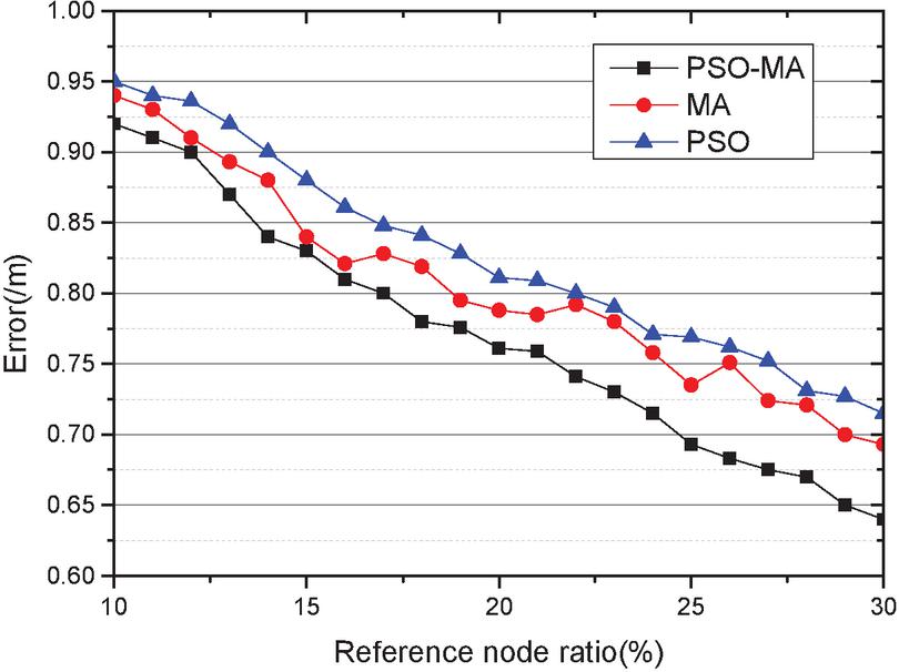
Figure 1 Comparison of the proportional positioning errors of the three algorithms at different reference nodes.

5.2 Comparison of Positioning Indicators

(1) Influence of reference node ratio
Figure 1 shows the results of the positioning errors of the three algorithms under different reference node ratios. From the figure, it is found that as the ratio of the reference nodes increases, the positioning errors of the three algorithms are gradually getting smaller, but algorithm PSO-MA performs better in the effect of positioning error, and the positioning accuracy is increased by 8.22% and 10.31% compared with the MA algorithm and the PSO algorithm, respectively. On the whole, the PSO-MA algorithm can effectively improve the positioning accuracy in terms of reference node ratio.

(2) Influence of node density
Figure 2 shows the results of the positioning errors of the three algorithms under different node densities. As the number of nodes gradually increases, the errors of the three positioning algorithms are reduced to varying degrees. Compared with the MA algorithm and the PSO algorithm, the positioning accuracy of the PSO-MA algorithm is improved by 9.42% and 11.34%, respectively. On the whole, the entire curve tends to stabilize, mainly due to the increase in node density, which increases the mutual communication between nodes. When the density of the area to be tested is small, the PSO-MA algorithm has obvious advantages and good stability, so the PSO-MA algorithm can effectively improve the positioning accuracy in terms of node density.

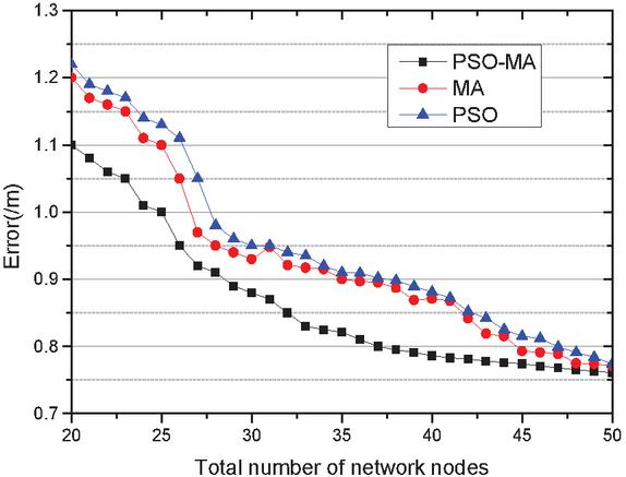
Figure 2 Comparison of the positioning errors of the three algorithms at different node densities.

(3) The influence of communication radius
Figure 3 shows the results of the positioning errors of the three algorithms under different communication radii. As the communication radius gradually increases, the positioning accuracy of the PSO-MA algorithm is increased by 7.5% and 10.5% compared to the MA and PSO algorithms, respectively. This shows that the communication radius has a greater impact on the positioning error. When the communication radius is small, the number of anchor nodes is small, which leads to unsatisfactory positioning effects. But the PSO-MA algorithm has higher accuracy than the MA and PSO algorithm. This shows that the size of the communication radius has little effect on the PSO-MA algorithm.

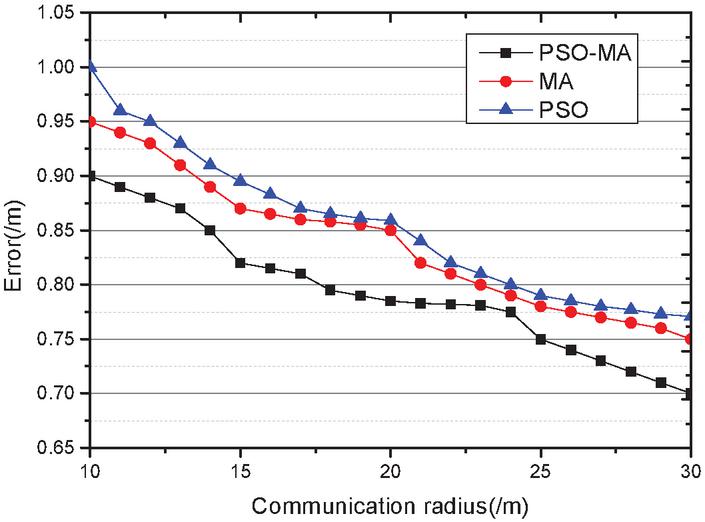
Figure 3 Comparison of positioning errors of the three algorithms under different communication radius.

6 Conclusion

Aiming at the shortcomings of large node location errors in wireless sensor networks, this paper proposes a node location algorithm based on the PSO-MA algorithm to analyze the causes of the errors. Under the analysis of the shortcomings of the performance of the PSO algorithm, the Laplace distribution is used to initialize the population and the particle weight is optimized. The dynamic guidance factor is used to update the individual position, and the Monkey Algorithm is used to select the individual. Compared with MA, the PSO-MA algorithm in the simulation experiment can effectively improve the accuracy of the node location.

Funding Statement

This work was supported in part by the National Natural Science Foundation of China (41701479), and in part by the Fundamental Research Funds in Heilongjiang Provincial Universities of China under Grant 135509136, and in part by the Fundamental Research Funds in Heilongjiang Provincial Universities of China under Grant 135309453. and in part by the Fundamental Research Funds of Qiqihar science and Technology Bureau(GYGG-201914)

References

[1] N. Yu, J.W. Wan, Y.F. Wu. ‘Localization algorithm in wireless sensor networks.’ Journal of Transduction Technology, Vol. 20, No. 1, pp. 187–192, January 2007.

[2] Yun S., Lee J., Chung W., et a1. ‘A soft computing approach to localization in wireless sensor networks.’ Expert System with Applications, Vol. 36, No. 4, pp. 7552–7561, April 2009.

[3] J.B. Xue and X.L. Chang. ‘WSN node localization based on artificial bee colony.’ Journal of Lanzhou University of Technology. Vol. 46, No. 3, pp. 94–99, March 2020.

[4] R. Zhang. ‘Study on Target Localization Algorithm in Wireless Sensor Networks.’ Chinese Journal of Sensors and Actuators, Vol. 31, No. 4, pp. 625–629, April 2018.

[5] M. Pang, Z.H. Feng, W.X. Bai. ‘DV-Hop node location algorithm optimized by improved artificial immune algorithms.’ Journal of Terahertz Science and Electronic Information Technology, Vol. 18, No. 6, pp. 1133–1140, June 2020.

[6] X. Zhang, Y.Y. Mao, P. Xu. ‘Node location algorithm based on distance optimization and improved particle swarm optimization.’ Computer Engineering and Design, Vol. 39, No. 7, pp. 1818–1822. July 2018.

[7] Z.A. Zhou, K. Xu, Q. Cheng et al. ‘Node localization of wireless sensor network by using artificial bee colony algorithm optimizing neural network.’ Journal of Nanjing University of Science and Technology, Vol. 41, No. 4, pp. 466–471, April 2017.

[8] Q.G. Gu. ‘Research on Support Vector Machine’s Mobile Node Positioning Based on Fisherman’s Fishing in WSN.’ Bulletin of Science and Technology, Vol. 32, No. 12, pp. 174–178, December 2016.

[9] H.X. Chen and L.M. Wang. ‘Sensor Node Localization Based on Artificial Bee Colony Algorithm Optimizing Support Vector Machine.’ Journal of Jilin University: Sci Ed, Vol. 55, No. 3, pp. 647–651 March 2017.

[10] J. Zhang, X. Guo and W. Li. ‘Research of WSN Node Localization Based on Fruit Fly Optimization Algorithm.’ Microelectronics & Computer, Vol. 35, No. 4, pp. 89–92, April 2018.

[11] Mohanta T.K., Das D.K. Class Topper Optimization Based Improved Localization Algorithm in Wireless Sensor Network[J]. Wireless Personal Communications, 2021: 1–20.

[12] Huang X., Han D., Cui M., et al. Three-Dimensional Localization Algorithm Based on Improved A* and DV-Hop Algorithms in Wireless Sensor Network[J]. Sensors, 2021, 21(2): 448.

Biographies

Wenli Liu received the bachelor’s degree in Mechanical design and manufacturing from North University of China in 2004, the master’s degree in Signal and information processing from North University of China in 2007. She is currently working as an lecturer at Qiqihar University. Her research areas include Signal and information processing, digital image processing and cloud computing.

Cuiping Shi received the bachelor’s degree in Communication engineering from Northeast Petroleum University in 2004, the master’s degree in Signal and information processing from Yangzhou University in 2007, and the engineering of doctorate degree in Electrical-Electronics & Computer Engineering from Harbin Institute of Technology in 2016, respectively. She is currently working as an Assistant Professor at Qiqihar University. Her main research interests include remote sensing image processing, pattern recognition, and machine learning. She has been serving as a reviewer for many highly-respected journals.

Hengjun Zhu received the bachelor’s degree in Electronics and information system from Heilongjiang University in 1991, the master’s degree in Communication and information system from Harbin Engineering University in 2007.He is currently working as an Professor at Qiqihar University. Her research areas include Signal and information processing.

Hongbo Yu received the bachelor’s degree in Electronic information engineering from Xi’an Institute of engineering and technology in 2003, the master’s degree in Electronic information engineering from Xi’an University of Technology in 2006. He is currently working as an Associate Professor at Qiqihar University. His research interests include cloud computing and digital signal processing.

Journal of Web Engineering, Vol. 20_4, 1075–1092.
doi: 10.13052/jwe1540-9589.2048
© 2021 River Publishers

Abstract

1 Introduction

2 Introduction to Node Location Based on DV-HOP

2.1 DV-HOP Algorithm

2.2 Error Analysis

3 PSO and the Analysis

3.1 Particle Swarm Optimization

3.2 Algorithm Insufficient Convergence Analysis

4 Node Location Based on PSO-MA

4.1 Population Initialization

4.2 Weight Optimization

4.3 Update of Individual Location

4.4 Selection of Individuals

4.5 Positioning Steps

5 Simulation Experiment

5.1 Performance Comparison

5.2 Comparison of Positioning Indicators

6 Conclusion

Funding Statement

References

Biographies