Convolutional Neural Networks Using Log Mel-Spectrogram Separation for Audio Event Classification with Unknown Devices

Soonshin Seo¹, Changmin Kim² and Ji-Hwan Kim^1,*

¹Dept. of Computer Science and Engineering, Sogang University, Seoul, Republic of Korea

²LG Electronics, Seoul, Republic of Korea

E-mail: ssseo@sogang.ac.kr; changmin0.kim@lge.com; kimjihwan@sogang.ac.kr

*Corresponding Author

Received 12 April 2021; Accepted 05 November 2021; Publication 07 January 2022

Abstract

Audio event classification refers to the detection and classification of non-verbal signals, such as dog and horn sounds included in audio data, by a computer. Recently, deep neural network technology has been applied to audio event classification, exhibiting higher performance when compared to existing models. Among them, a convolutional neural network (CNN)-based training method that receives audio in the form of a spectrogram, which is a two-dimensional image, has been widely used. However, audio event classification has poor performance on test data when it is recorded by a device (unknown device) different from that used to record training data (known device). This is because the frequency range emphasized is different for each device used during recording, and the shapes of the resulting spectrograms generated by known devices and those generated by unknown devices differ. In this study, to improve the performance of the event classification system, a CNN based on the log mel-spectrogram separation technique was applied to the event classification system, and the performance of unknown devices was evaluated. The system can classify 16 types of audio signals. It receives audio data at 0.4-s length, and measures the accuracy of test data generated from unknown devices with a model trained via training data generated from known devices. The experiment showed that the performance compared to the baseline exhibited a relative improvement of up to 37.33%, from 63.63% to 73.33% based on Google Pixel, and from 47.42% to 65.12% based on the LG V50.

Keywords: Audio event classification, unknown device, log mel-spectrogram, log mel-spectrogram separation, convolutional neural networks.

1 Introduction

The widespread application of multimedia has resulted in the increase of the size of the solo creator market, and personal video media production and distribution became easier. Although multimedia still relies on metadata to interpret overflowing video media information, research to automatically analyze the meaning of text, image, and audio information in video is being actively conducted owing to advances in machine training. Audio information analysis is largely divided into speech recognition, which analyzes the speech signal from a person’s mouth and converts it into a character string, and audio event classification, which detects and classifies non-verbal signals such as dog and car horn sounds. In addition to analyzing video information, audio event classification is a technology that can indicate what type of sound is currently being produced by classifying various ambient sounds occurring in daily life on behalf of the human ear. It is possible to assist people with limited ambient sound information, such as modern people who usually wear earphones or people with hearing impairments, to evaluate the situation and have an immediate response in dangerous situations.

1.1 Acoustic Scene Classification

Deep neural networks (DNNs), which have recently attracted attention in the field of machine training, have been applied to speech recognition and image classification, showing excellent performance improvement [1, 2]. DNN-based algorithms have also been studied for audio event classification problems [3]. Among them, a method of visualizing audio data as a two-dimensional (2D) image, called a spectrogram, and training it with a convolutional neural network (CNN) suitable for an image classification problem is widely used [4]. The spectrograms are expressed on the time and frequency axes. To generate a spectrogram, the frequency energy must be extracted using a Fourier transform, while a window of a certain length moves with respect to the original data containing time and amplitude information.

Figure 1 shows a spectrogram. For clock alarm audio data with a sampling rate of 16000 and a length of 0.4 s, a window size of 640 frames and a window movement distance of 163 frames were used. The x-axis represents time, and the y-axis represents the frequency. Each pixel contains a dB value for each frequency. The strongest energy is set to 0 and expressed in white. As the energy becomes weaker, the dB value decreases and becomes darker.

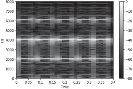
Figure 1 Spectrogram.

Figure 2 shows the structure of the audio event classification system, in which the spectrogram is used as an input to the audio event classification system. The input spectrogram starts with the input layer of the CNN, passes through the convolutional layer, and becomes a plurality of filter images. Finally, in the dense layer or the global average value pooling layer, a spectrogram is classified using information on a plurality of filter images, and a softmax value is output.

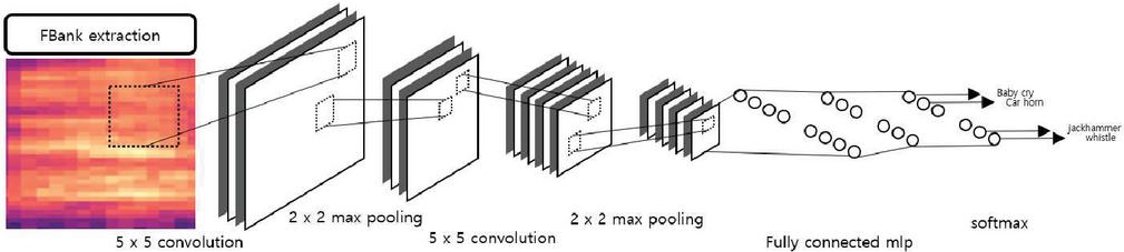
Figure 2 Structure of audio event classification system.

1.2 Performance of Audio Event Classification on Unknown Devices

There are various problems to be solved in the classification of audio events; however, in this study, we focused on the result of poor performance when the device recording data used for training and that used for testing are different. For example, the American Institute of Electrical and Electronics Engineers hosted a world-class Detection and Classification of Acoustic Scenes and Events (DCASE) challenge to address various topics related to audio event classification. The audio input device used to record the training data and that used to record the test data were the same. As a result, for the problem of classifying 10 scenes, the team that recorded 85.2% won the first place [5].

In the same year, in Task 1B: acoustic scene classification with mismatched recording devices, test data were recorded using a device other than the audio input device used to record the training data. Similarly, for the problem of classifying 10 scenes, the team with 75.3% won first place [6]. It was found that there is a large difference in performance when the same device is used for training and recording and when different devices are used. Here, the device used for training and recording is called a known device, whereas the device only used for recording is called an unknown device.

To determine why the performance of an unknown device is poor, we first analyzed the waveform of the data recorded with various input devices. As a result of analyzing the frequency range emphasized by the device used for recording, spectrograms were generated by the known and unknown devices, and it was observed that the spectrograms made with the unknown devices had different features.

Figure 3 shows spectrograms extracted after recording through various devices for the same audio data input. Audio data with a sampling rate of 16000 and a length of 0.4 s were recorded on four devices: iPhone SE, Google Pixel, Samsung Galaxy S9, and LG V50. The spectrogram of the data recorded by the iPhone SE is shown in the upper left corner. Three lines were highlighted around 2000 Hz, 4000 Hz, and 6000 Hz. Thus is the only one of the four devices, in which the area around 3000 Hz is represented by a black area. In the spectrogram of the Google Pixel located in the upper right, strong energy is observed at approximately 2000 Hz, but at 4000 Hz, the energy is weaker than that of the iPhone SE, and noise is mixed, hindering visualization. The LG V50 at the bottom right had noise input between 6000 Hz and 8000 Hz, which is the high-frequency range. Even if the same data are recorded, the shape of the spectrogram may be slightly different for each device.

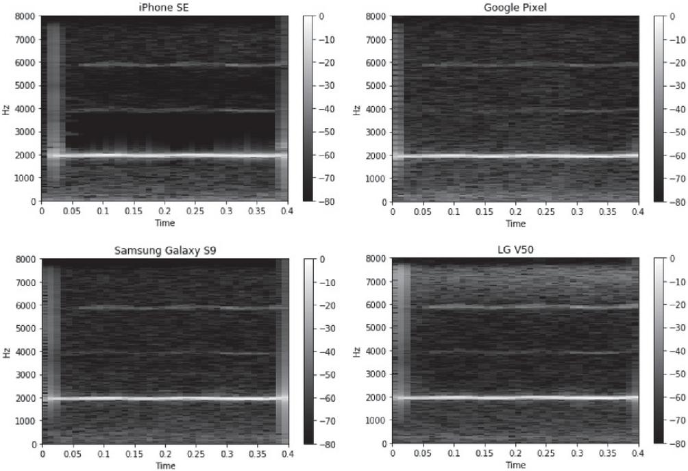
Figure 3 Spectrograms recorded and extracted by various devices for the same input.

1.3 Contributions

When transplanted to an unknown device using the CNN-based audio event classification model [4], the performance was very poor at 63.63% for Google Pixel and 47.42% for LG V50. In this study, the difference in performance between known and unknown devices was because the shape of the spectrogram for each device was partially different, and the spectrogram had different characteristics from the image. As the frequency domain to be emphasized is different for each audio input device, even in the case of an image, a specific area may be more emphasized for each camera device that converts an image into data.

However, the meaning of the image is not different, regardless of where the object appears in the image. For example, when a dog appears at the top or at the bottom of an image, the position in the image is different, but the presence of the dog in the picture is a fixed characteristic. Therefore, in image classification, even if a specific area of an image is erased, it is possible to identify and classify the necessary information in another location.

However, because the spectrogram has a fixed frequency axis, high- and low-pitched audio events are located at the top and bottom of the spectrogram, respectively. If a specific area of the spectrogram extracted from data recorded by a device is not highlighted, information appearing only in that specific area cannot be obtained through the recording device. Therefore, in this study, we used a log mel-spectrogram, which can show the characteristics in more detail than the mel-spectrogram in the low- and high-frequency regions.

In addition, because spectrograms have different characteristics from images, the CNN used for image classification should be used in accordance with the characteristics of the spectrogram in the audio event classification problem. McDonnell’s team, which won second place in the DCASE Task 1B held in 2019, divided the log mel-spectrogram into high- and low-frequency regions to reflect the characteristics of images and other spectrograms, which has been applied to input CNNs [7]. Thus, in this study, the feature parameter separated from the log mel-spectrogram was applied to the audio event classification problem.

Furthermore, in the spectrogram, the meaning of the parameter used for the x-axis and that used for the y-axis differ in the time and frequency bands, respectively. Therefore, to determine whether time or frequency information should be reflected in training, we experimented on strides in the pooling layer to generate a better performance audio event classification CNN structure. As a result, the performance compared to the previous study [4] showed a relative improvement of up to 37.33%, from 63.63% to 73.33% based on Google Pixel, and from 47.42% to 65.12% based on LG V50.

1.4 Paper Organization

Section 2 introduces various feature parameters used in audio event classification, feature parameter separation methods, and training models. Section 3 describes a CNN using the log mel-spectrogram separation applied in the proposed audio event classification. In Section 4, the effect of the log mel-spectrogram application, log mel-spectrogram separation, and the proposed CNN model is tested on servers and embedded devices, and the degree of performance improvement is evaluated through comparison with existing studies. Section 5 provides the conclusions of this study.

2 Related Works

Section 2.1 describes various spectrograms used in the audio scene and audio event classification problems. Section 2.2 describes the attempts to train by separating the spectrogram, and Section 2.3 describes the existing research on an audio event classification model based on CNNs.

2.1 Previous Methods on Feature Parameters in Audio Event Classification

The spectrograms used in DCASE Task 1: Acoustic scene classification challenge include Constant-Q spectrogram [8], mel frequency cepstral coefficients (MFCCs) [9], and log mel-spectrogram [10]. This challenge focused on an audio scene classification problem that was slightly different from the definition previously discussed in this paper. The 10-s long data should be classified, including continuous events such as department store, park, and subway station environment sounds, and not input from short events such as dog barking and car horn sounds. The Brno University of Technology team using the Constant-Q spectrogram was ranked third among the 24 teams participating in DCASE 2018 [8]. Figure 4 shows a visualization of the Constant-Q spectrogram.

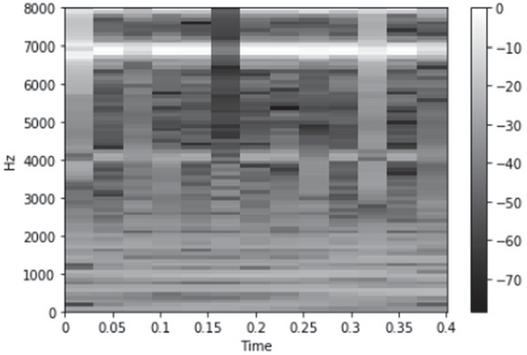
Figure 4 Constant-Q spectrogram.

The MFCCs, which are often used in speech recognition, are also used in audio scene classification problems. Dorfer et al. won second place in the challenge of the same year using MFCCs [9]. For clock alarm audio data such as Constant-Q, the moving distance of the window was set to 160. Figure 5 shows the spectrogram of the MFCCs.

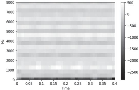
Figure 5 MFCCs spectrogram.

The spectrogram used in the model that won first place was the log mel-spectrogram. Sakashita et al. used an ensemble of nine CNN models using log mel-spectrograms [10]. Figure 7 shows a picture of the log mel-spectrogram, which is the same as the audio data used in Constant-Q and MFCCs, and the window size and moving distance are the same as those of the MFCCs. Visually, the frequency ranges around 4500 Hz, 6500 Hz, and 7500 Hz are emphasized, showing a remarkable effect.

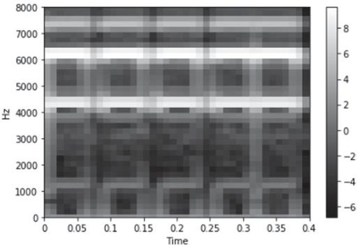
Figure 6 Log mel-spectrogram.

Later, in the same challenge of DCASE 2019, Chen et al., who used the rogue mel-spectrogram, won the first place. In DCASE 2020, all of the top 10 systems in Task 1A: acoustic scene classification with multiple devices used log mel-spectrograms to reduce the performance gap between devices, and were evaluated as a spectrogram suitable for audio scene classification problems. A mel-spectrogram is used to classify audio events [4], and is similar to the log mel-spectrogram, which has the best performance in the current audio scene classification problem. When a log scale is applied to the mel-spectrogram, it becomes a log-spectrogram.

Lee et al. addressed the issue of classifying 30 audio events using mel-spectrogram and VGGNet in 2017. The authors obtained an accuracy of 81.5% for the UrbanSound8k, BBCSoundFX, DCASE2016, and FREESOUND datasets. Figure 7 shows the mel-spectrogram used in Lee’s study extracted under the same conditions for the clock alarm audio data previously mentioned. Similar to the log mel-spectrogram, it is heavily emphasized around 4500 Hz and 6500 Hz, and other areas are darker.

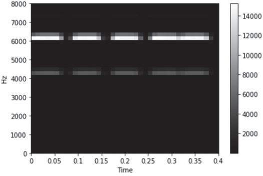
Figure 7 Mel-spectrogram.

2.2 Previous Methods on Feature Parameters Separation in Audio Event Classification

Piczak et al. used a technique for separating MFCCs in the problem of classifying datasets ESC-50 [11], ESC-10 [11], and UrbanSound8K [12] in 2015. The effectiveness of the audio event classification problem has been evaluated [13]. In 2017, they participated in the DCASE to evaluate how the resolution of the separated spectrogram affects the classification of audio events [14]. Phaye et al. proposed a CNN model with mel-spectrogram separation for the first time in 2019 [15]. In the challenge for classifying audio scenes using unknown devices, McDonnell et al. won second place at DCASE 2019 using a CNN model separated from a log mel-spectrogram [7]. Suh et al. won the first place in DCASE 2020 by outputting a log mel-spectrogram in 256 orders and dividing the low-frequency band into three divisions into 64th, 64th, and 128th orders [16].

2.3 Previous Methods on Neural Networks in Audio Event Classification

The first training model introduced in the field of audio event classification was the hidden Markov model-support vector machine [17]. Later, with the advent of DNNs, a training model using feedforward neural networks was proposed [3]. Recently, among DNNs, many studies have been conducted using CNNs, which have excellent performance in image recognition. Representative examples of CNNs include VGGNet [18], ResNet [19] and GoogleNet [20]. In particular, an audio signal classification system with a small model complexity of 81.5% using VGGNet [18] was proposed [4].

3 Convolutional Neural Networks Using Log Mel-Spectrogram Separation

As mentioned in Section 2, the mel-spectrogram was used for the audio event classification problem. However, in the audio scene classification problem of the DCASE 2020 challenge, an increasing number of teams used log mel-spectrograms, and their performance is improved every year. We extracted and compared the mel- and log mel-spectrograms from the audio event. Figure 8 shows the appearance of mel-spectrograms extracted from two crying babies, indicating that the characteristics of the sounds mainly appear between 5000 Hz and 7000 Hz.

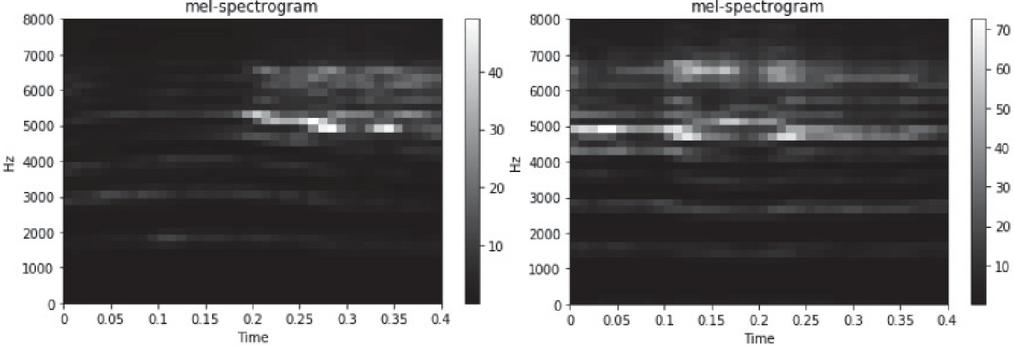
Figure 8 Mel-spectrograms extracted from two crying babies.

Figure 9 shows a collection of log mel-spectrograms extracted from the same two crying babies. In the log mel-spectrogram, the characteristics of the sounds are evident even at frequencies between 5000 and 7000 Hz.

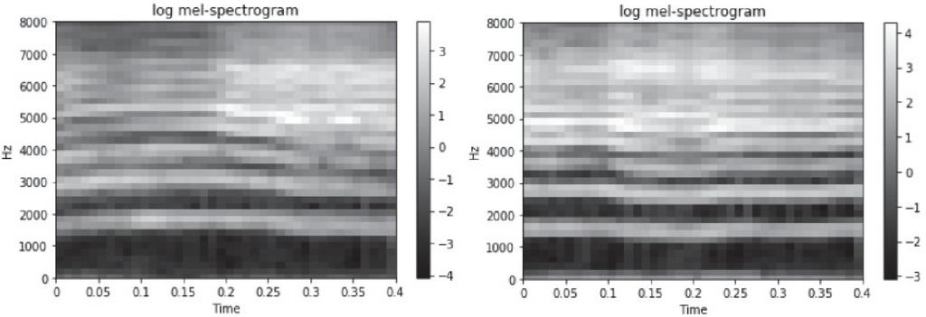
Figure 9 Log mel-spectrograms extracted from two crying babies.

The method used to draw the log mel-spectrogram is as follows: the input audio signal is sampled at 16 kHz, 2 bytes per sample, and consists of a mono channel. A short time Fourier transform is performed while the Hamming window of 640 frames moves in units of 160 frames with respect to the input signal. One feature value is extracted for each triangle bin by multiplying the weight for each frequency energy and covering all the windows with a triangle bin that increases on the mel scale. A filter bank feature parameter is generated by composing these feature values into one vector. The generated filter banks are arranged on the time axis to generate a 2D image, which is a mel-spectrogram.

Additionally, a log mel-spectrogram is generated by applying a log scale. Log mel-spectrogram separation is a method of passing the decomposed feature parameters through a CNN model and combining them in the final global mean pooling layer step. The log mel-spectrogram separation algorithm proposed in this study is based on the method of McDonnell et al., who won second place in the DCASE 2019 Task 1B [7]. The use of a CNN algorithm by interpreting the spectrogram as an image is a good method to improve performance in audio event classification. In image recognition, objects are classified by the same image label that is at the top or bottom. However, in the spectrogram, there is a difference in frequency between the top and bottom, thus the meaning of the feature is different when the feature is at the top and bottom. After passing the 40th order filter bank through the CNN model for each 20th order, the log mel-spectrogram is separated. As a result, information on the spectrogram of the low- and high-frequency bands can be separately trained.

In addition to the audio scene and audio event classification problems, the characteristics of images and other spectrograms should be considered. The proposed CNN has three major changes from the VGGNet-based CNN [4], which was used for audio event classification in the previous study by Lee et al. Each dense layer was a global average value-pooling layer, and maximum value pooling was used. With average value pooling, the time-axis stride was changed from one to two. The global average value pooling layer uses the average value pooling of the first layer instead of the dense layer of three layers used in the existing CNN classifier, and uses the abstracted features as a classifier through the convolutional layer. This was first proposed by Line et al. [21] and applied to Google’s Inception Net [22].

Compared to the dense layer, the number of parameters can be reduced, and the location information is not removed. Based on the existing model, approximately 15 million parameters can be reduced to 540,000. The average value pooling layer takes the average of the values in the receptive field. Compared to the maximum value pooling that takes the largest value, training is not adequately performed when used with the ReLU activation function in a deep CNN, but overfitting does not occur [23]. The CNN model used in this study uses ReLU, but it is not deep, and is vulnerable to overfitting in solving the performance difference between devices. Thus, the average value pooling layer was used.

In addition, the stride of the time axis was set to two in the average value pooling layer. As a result, the time axis length of the input spectrogram feature decreased by half each time the average value pooling layer was passed. In the case of this system, an image of (40,40) size consisting of 40 frequency information and 40 time information was input and had two strides (1,2) in average value pooling layers, thus the image was reduced up to the (40,10) dimension. We experimented with the (40,20) and (40,5) dimensions by varying the number of strides in the average pooling layer, but the best performance was in the (40,10) dimension.

The structure of a CNN using log mel-spectrogram separation is shown in Figures 10 and 11. The (40,40)-dimensional spectrogram was divided into two log mel-spectrograms of (40,20) dimension using a lambda function. Two log mel-spectrograms of (40,20) dimensions were used as inputs for the CNN. A 2D convolutional layer was used after batch normalization. In the convolutional layer, the size of the kernel was (3,3), the stride was (1,1), and zero padding was used to make the input and output dimensions the same. The number of filters started at 18 and was doubled each time the convolutional layer was repeated.

After the two convolutional layers, the average value in the kernel of size (2,2) was extracted using the average value pooling layer. We used zero padding, whereas the stride used (2,1), thus the dimension was cut in half for an axis with a stride of 2. Two convolutional layers and one average value pooling layer were repeated twice. Two convolutional layers and an average value pooling layer were used. The average value pooling layer used strides (1,1) to prevent dimension reduction. As a result, when passing through each path, the dimension was from (40,20) to (10,20), and the number of filters was 288. The two paths were merged into a (10,40) dimension, followed by a convolutional layer, and finished with a global average pooling layer.

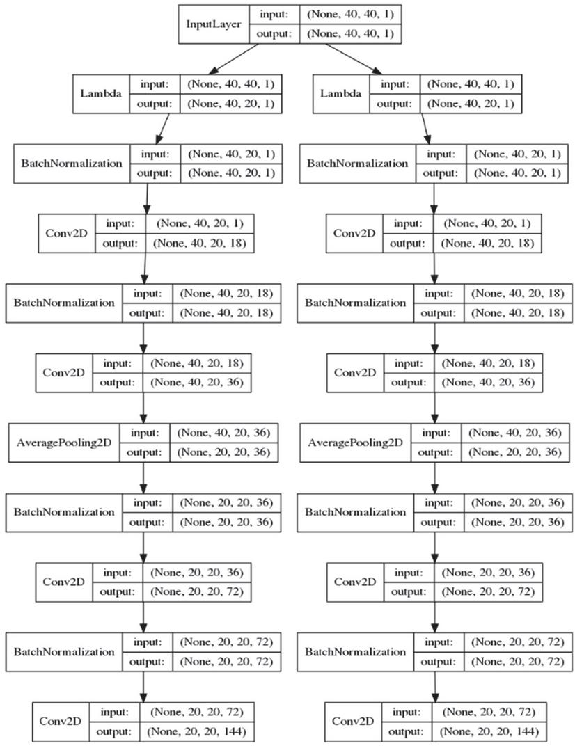
Figure 10 Proposed CNN structure using log mel-spectrogram separation (1).

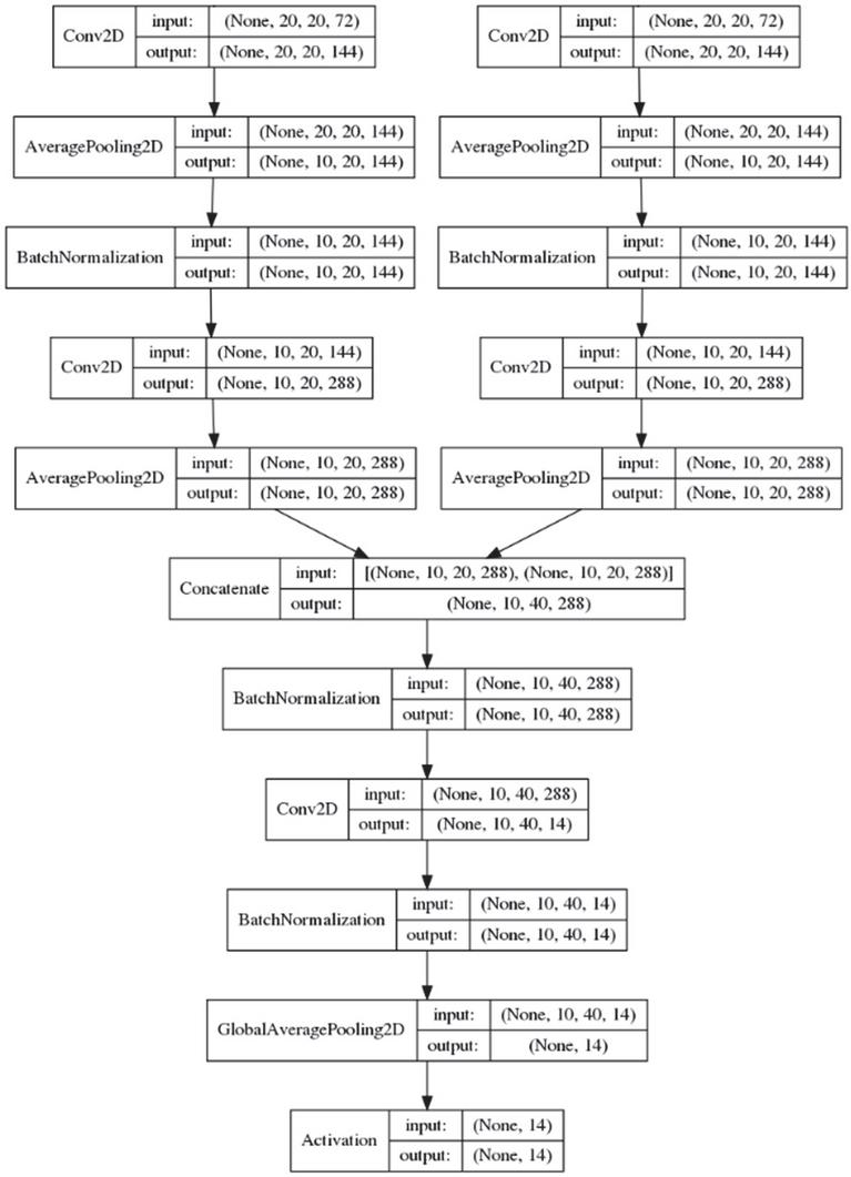
Figure 11 Proposed CNN structure using log mel-spectrogram separation (2).

4 Experiments

Section 4 describes the experiments and their evaluation. Section 4.1 describes the construction of datasets used for training, testing, and verification. Section 4.2 describes the experimental configurations. Section 4.3 describes the experimental results on the server to verify the effect of the log mel-spectrogram, the effect of the proposed CNN, and the effect of the CNN using the log mel-spectrogram separation. Section 4.4 describes the improvement the performance of an unknown device compared to previous research [4] by implementing an audio event classifier for real-time embedding.

4.1 Dataset Setup and Data Pre-processing

A total of 16 classes were selected: 13 dangerous signal classes, including fire alarm, siren, dog barking, car horn, bicycle horn, glass cracking, water boiling, water kettle whistle, human screaming, baby crying, jackhammer, car passing, and whistling sounds; and 3 types of information signal classes, including the sound of an electronic clock alarm, the sound of a door knock, and the sound of human speech. These sounds can result in problems if not recognized by a person with a hearing-related physical function is not recognized.

According to Grice et al., the time taken for humans to respond to and evaluate audio signals is an average of 0.386 s, with a standard deviation of 0.052 s [24]. Because the response speed of the real-time audio event classifier is influenced by the input length of the audio event, the input length was set to 0.4 s in this study to implement a real-time audio event classifier with a performance similar to that of humans.

Data collection sources included Google audio set [25], UrbanSound8k [12], BBC Sound FX [26], DCASE 2016 Task 1 data set [27], and Freesound. Google audio sets are publicly available data such as to provide an event sound database that can be used as a realistic evaluation index for audio event search problems. Each data consisted of a 10-s long audio clip that was directly separated by a human from a YouTube video. There was total of 632 types, 2,084,320 sheep. In this study, it was used as the main source of data for the sound of bicycle horns and screams.

UrbanSound8K is audio event data collected and distributed by the New York University, and audio data collected from www.freesound.org were cut and tagged to fit the event section. One audio sample consisted of less than 4 s and was provided as a total of 8,732 files. The audio sample had 10 audio event classes and a total length of 9 h. The UrbanSound8K dataset contains 10 types of audio events.

BBC Sound FX data is a collection of sound events used in cities/TV broadcasts and consists of 40 CDs. For all tracks, manual tagging was freely performed without limiting direct events, and 160 audio events existed as a result of tagging. Among them, the top 10 audio events based on frequency were selected and included in the training materials. BBC Sound FX has 10 audio events.

DCASE is a challenge to evaluate the audio classification performance for four tasks. Among them, Task 1 contained many of the events selected in the previous section for the classification of audio scenes. Like UrbanSound8K, it was used as training data as a refined dataset without the need for separate tagging. It is a database in which random users share sounds with known keywords on the cloud.

When constructing a class from the previous three datasets, duplicate events exist; therefore, data were collected from freesound.org to compensate. Because the collected data may contain errors, the section where the actual sound exists was manually tagged. Data were collected directly from freesound.org and YouTube for classes that were not included in the dataset or were insufficient in quantity, such as the sound of a clock alarm, boiling water, glass breaking, and whistling of a kettle. The amount of data collected is listed in Table 1.

Table 1 Information of collected data

Class	Size (byte)	Files	Duration	Source
Baby cry	115,475,918	54	60.14	Urbansound8k
Bicycle horn	21,320,874	91	11.10	Google audio set
Boiling	855,504,430	51	44.53	YouTube, Freesound
Car horn	45,356,560	369	23.61	Urbansound8k
Car passing	12,188,972	42	6.35	YouTube, Freesound
Clock alarm	13,770,660	43	7.17	YouTube, Freesound
Dog bark	44,382,322	362	23.11	Urbansound8k
Door knock	10,728,150	69	5.59	Urbansound8k
Fire alarm	8,594,532	20	4.48	YouTube, Freesound
Glass break	11,817,608	13	6.15	YouTube, Freesound
Jackhammer	116,567,496	1000	60.69	Urbansound8k
Kettle whistle	47,451,994	10	24.71	YouTube, Freesound
Scream	18,384,972	106	9.57	Google audio set
Siren	117,197,132	929	61.02	Urbansound8k
Whistle	26,095,484	40	13.59	YouTube, Freesound
Speech	57,551,044	196	29.97	Manually recordings

Figure 12 Waveform of sound source before data pre-processing.

Data pre-processing was performed as follows: when the collected data were cut by 0.4 s, there was a section where no audio event existed. Figure 12 shows the source of audio data for dog barking. It can be seen that the data corresponding to the dog’s barking sound are not filled with the corresponding audio event. To solve this problem, a section lower than a certain threshold for the average energy value was removed. The threshold values were set differently according to the characteristics of each class. As a result, silence was removed, as shown in Figure 13.

Figure 13 Waveform of sound source after data pre-processing.

As a result of data pre-processing, the length of the glass cracking sound, which was the smallest class, was reduced from 6.15 min to 3 min. To balance the amount of data between the classes, the other classes were also set to a 3-min length equal to the length of the glass breaking sound. As a result of experimenting using this as training data, a low performance of 67.02% was obtained based on LG V50. The training data were augmented by re-recording the existing data for Samsung Galaxy S9, iPhone SE, LG V50, and Google Pixel. With the addition of the devices, the performance significantly increased.

4.2 Experimental Configurations

The training and experimental data were divided as follows: 412 data in length of 0.4 s $\times$ 16 classes of audio data divided into 5 folds (82 data per fold $\times$ 16 classes). 4 folds were re-recorded through Samsung Galaxy S9 and iPhone SE devices (known devices) and used as training data for 3 devices $\times$ 412 data $\times$ 16 classes. The other fold was re-recorded using Samsung Galaxy S9, iPhone SE, Google Pixel, and LG V50 devices (55 devices $\times$ 82 data $\times$ 16 classes). The data re-recorded on Samsung Galaxy S9 and iPhone SE is a verification set (22 devices $\times$ 82 data $\times$ 16 classes), Google Pixel, LG V50 (unknown device) was used as a test set (2 devices $\times$ 82 data $\times$ 16 classes).

The accuracy of the test set was measured based on the model with the highest accuracy for the verification sets of Samsung Galaxy S9 and iPhone SE devices, and the performances of Google Pixel and LG V50 in the test sets were evaluated. Librosa was used for the feature extraction. Librosa is a Python package used to analyze audio signals and music. Spectrogram, Constant-Q, mel-Spectrogram, and MFCCs can be easily extracted, thus they are used in various auditory intelligence studies such as speech recognition, music recognition, speaker recognition, and audio event classification. The version of the Librosa used in this study was 0.7.1. The Python libraries used for training included numpy 1.16.4, keras 2.2.4, and tensorflow 1.12.0. The Adam method was used as an optimizer. The loss function used sparse categorical cross-entropy, and the metrics were accurate. The generation (epoch) used was 15. The existing research model is an audio event classifier based on the CNN proposed by Lim in 2018. A mel-spectrogram was used as the feature parameter. The model uses a CNN based on VGGNet. Feature parameter separation was not used, and (1,1) was used for the stride in the pooling layer.

4.3 Experimental Results of CNNs Using Log Mel-spectrogram Separation

The same training and test data were used to compare the performance of the mel- and log mel-spectrograms, and the model was matched with the CNN used in the previous study. As shown in Table 2, the average accuracy compared to the mel-spectrogram increased to 4.46% for Google Pixel and 8.68% for LG V50.

Table 2 Experimental results of applying log mel-spectrogram (accuracy, %)

	Mel-spectrogram		Log mel-spectrogram

	Baseline CNN		Baseline CNN

	w/o Spectrogram Separation		w/o Spectrogram Separation

Conditions	Google Pixel	LG V50	Google Pixel	LG V50
Fold 0	81.48	72.82	88.33	77.18
Fold 1	86.14	73.87	87.42	78.31
Fold 2	82.24	71.27	86.59	79.73
Fold 3	81.33	64.79	87.58	80.95
Fold 4	83.92	70.2	87.5	80.18
Average	83.02	70.59	87.48	79.27

To compare the performance of the conventional CNN and the proposed CNN, the same training and test data were used, and the feature parameter extraction method was a log mel-spectrogram. As shown in Table 3, the average accuracy compared to the conventional CNN increased by 6.69% for Google Pixel and 9.70% for LG V50.

Table 3 Experimental result of the proposed convolutional neural network (accuracy, %)

	Log mel-spectrogram		Log mel-spectrogram

	Baseline CNN		Proposed CNN

	w/o Spectrogram Separation		w/o Spectrogram Separation

Conditions	Google Pixel	LG V50	Google Pixel	LG V50
Fold 0	88.33	77.18	94.65	90.59
Fold 1	87.42	78.31	95.03	93.00
Fold 2	86.59	79.73	95.73	92.53
Fold 3	87.58	80.95	96.04	92.07
Fold 4	87.50	80.18	95.20	91.84
Average	87.48	79.27	95.33	92.01

To determine the degree of reduction in performance difference between Google Pixel and LG V50 according to the application of log mel-spectrogram separation, we used log mel-spectrogram as the feature parameter extraction method and the proposed CNN as the model. As shown in Table 4, the accuracy difference between Google Pixel and LG V50 decreased from 3.32% to 3.16%, as the accuracy decreased by 0.06% in Google Pixel, but increased by 0.11% in LG V50.

Table 4 Experimental results of applying log mel-spectrogram separation (accuracy, %)

	Log mel-spectrogram		Log mel-spectrogram

	Proposed CNN		Proposed CNN

	w/o Spectrogram Separation		w/o Spectrogram Separation

Conditions	Google Pixel	LG V50	Google Pixel	LG V50
Fold 0	94.65	90.59	95.86	91.57
Fold 1	95.03	93.00	93.90	91.64
Fold 2	95.73	92.53	95.43	91.77
Fold 3	96.04	92.07	95.43	91.84
Fold 4	95.20	91.84	95.73	93.75
Average	95.33	92.01	95.27	92.11

4.4 Experimental Results of Audio Event Classification in Embedded Devices

When an untrained type of sound is given, if there is no unknown class, the most similar sound among the 16 classes is output. Therefore, a state that does not belong to any of the 16 classes defined in the server audio event classifier must also be defined as one class. A total of 17 classes of audio event classifiers were obtained by training the daily noise data that are generally input for the four models. We used several methods for embedded devices, as described below.

TarsosDSP. It is a Java library for Android designed to analyze audio signals. It aims at easy-to-use and practical data processing. A fast Fourier transform was performed using 16 kHz, 16 bits per sample, mono channel, and signed big Indian audio signal using a window length of 40 ms, a window shift of 10 ms, and a window type using a Hamming window. Like Librosa, 40 triangular bins that increase in mel scale are covered to extract one feature value from each triangular bin to create a 40th filter bank and a mel-spectrogram with 40 time bins as one input, and then log scale. TarsosDSP is a library that is no longer under management since 2017. Thus, it could be a problem depending on the installation environment, being necessary to call the center frequency value that adjusts the mel scale when extracting the filter bank.

TensorflowLite. Extensions such as h5 and ckpt, which are model files used in the server, cannot be used in Android, which is a Java environment. TensorflowLite must be changed to a tflite extension. TensorflowLite is an end-to-end open-source platform for machine training [28]. Until 2019, debugging was difficult in the process of converting and applying the tflite extension, but in 2020, Tensorflow was registered in the Keras built-in function, enabling to solve various problems that occur during the model porting process. Converting the model reduces the file size and introduces optimizations that do not affect the accuracy. The TensorflowLite converter provides options to reduce the file size and accelerate execution. TensorflowLite provides a converter that converts the already trained Tensorflow model to TensorflowLite format, that is, tflite, in the form of Python application programming interface. The use of a TensorflowLite converter can reduce the size of the model and the time required for inference by reducing the precision of the values and operations in the model. Most models are converted in a direction that minimizes the loss of accuracy. TensorflowLite supports the reduction of the precision of values from the full floating point (float32) to semi-float (float16) or 8-bit integer values, and this affects the size and accuracy of the model, considering the computing power of the embedded device to be used. It also minimizes the reduction in model accuracy.

When testing with embedded devices, we evaluated he improvement in performance provided by the proposed system compared to the existing system. Similar to the experiment on the server, we used 412 data of 0.4 s in length for each class, 2636 s of audio data, 80% for training (2105 s), and 20% for testing (531 s). As shown in Table 5, the performance of Google Pixel and LG V50, selected as unknown devices, improved from 63.63% on Google Pixel to 73.33% compared to the previous study [4]. It also improved from 47.42% based on LG V50 to 65.12%.

Table 5 Experimental results in embedded devices (accuracy, %)

Baseline System		Proposed System
Google Pixel	LG V50	Google Pixel	LG V50
63.63	47.42	73.33	65.12

5 Conclusions

There audio event classification performance was identified to deteriorate in unknown devices. It was noted that the shape of the spectrogram was different for each device, and that the spectrogram had different characteristics from the image. Therefore, we used a log mel-spectrogram that can evenly show the characteristics in the low- and high-frequency regions. The feature parameter separated from the log mel-spectrogram was used as the input for the CNN. Because spectrograms have different characteristics from images, the CNN used for image classification was improved to solve the audio event classification problem. As a result, the performance compared to the previous research improved from 83.02% to 95.27% based on Google Pixel and from 70.59% to 92.11% based on LG V50. In addition, the experiment result of making an audio event classifier for embedded devices was improved from 63.63% to 73.33% based on Google Pixel and from 47.42% to 65.12% based on LG V50.

Acknowledgements

This work was supported by the Institute of Information & Communications Technology Planning & Evaluation (IITP) grant funded by the Korea government (MSIT) (1711103127, Development of Human Enhancement Technology for auditory and muscle support).

References

[1] G. Hinton, L. Deng, D. Yu, G. Dahl, A. Mohamed, N. Jaitly, and B. Kingsbury, “Deep neural networks for acoustic modeling in speech recognition: The shared views of four research groups,” IEEE Signal Processing Magazine, vol. 29, no. 6, pp. 82–97, 2012.

[2] D. Ciregan, U. Meier, and J. Schmidhuber, “Multi-column deep neural networks for image classification,” in Proceedings of IEEE Conference on Computer Vision and Pattern Recognition, pp. 3642–3649, 2012.

[3] M. Lim, and J. Kim, “Audio event classification using deep neural networks,” Phonetics and Speech Sciences, vol. 7, no. 4, pp. 27–33, 2015.

[4] M. Lim, D. Lee, H. Park, Y. Kang, J. Oh, and J. Kim, “Convolutional neural network based audio event classification,” KSII Transactions on Internet and Information Systems, vol. 12, no. 6, pp. 2748–2760, 2018.

[5] H. Chen, Z. Liu, Z. Liu, P. Zhang, and Y. Yan, “Integrating the data augmentation scheme with various classifiers for acoustic scene modeling,” arXiv preprint arXiv:1907.06639, 2019.

[6] M. Kosmider, “Calibrating neural networks for secondary recording devices,” in Proceedings of Detection and Classification of Acoustic Scenes and Events Workshop, pp. 25–26, 2019.

[7] M. McDonnell, and W. Gao, “Acoustic scene classification using deep residual network with late fusion of separated high and low frequency paths,” Technical Report of Detection and Classification of Acoustic Scenes and Events Challenge, 2019.

[8] H. Zeinali, L. Burget, and J. Cernocky, “Convolutional neural networks and x-vector embedding for DCASE2018 acoustic scene classification challenge,” arXiv preprint arXiv:1810.04273, 2018.

[9] M. Dorfer, B. Lehner, H. Eghbal-zadeh, H. Christop, P. Fabian, and W. Gerhard, “Acoustic scene classification with fully convolutional neural network and i-vectors,” Technical Report of Detection and Classification of Acoustic Scenes and Events Challenge, 2018.

[10] Y. Sakashita, and M. Aono, “Acoustic scene classification by ensemble of spectrograms based on adaptive temporal divisions,” Technical Report of Detection and Classification of Acoustic Scenes and Events Challenge, 2018.

[11] K. Piczak, “ESC: Dataset for environmental sound classification,” in Proceedings of the ACM International Conference on Multimedia, pp. 1015–1018, 2015.

[12] J. Salamon, C. Jacoby, and J. Bello, “A dataset and taxonomy for urban sound research,” in Proceedings of ACM International Conference on Multimedia, pp. 1041–1044, 2014.

[13] K. Piczak, “Environmental sound classification with convolutional neural networks,” in Proceedings of Machine Training for Signal Processing Workshop, pp. 1–6, 2015.

[14] K. Piczak, “The details that matter: Frequency resolution of spectrograms in acoustic scene classification,” Technical Report of Detection and Classification of Acoustic Scenes and Events Challenge, 2017.

[15] S. Phaye, E. Benetos, and Y. Wang, “Subspectralnet using sub-spectrogram based convolutional neural networks for acoustic scene classification,” in Proceedings of International Conference on Acoustics, Speech and Signal Processing, pp. 825–829, 2019.

[16] S. Suh, S. Park, Y. Jeong and T. Lee, “Designing acoustic scene classification models with CNN variants,” Technical Report, Detection and Classification of Acoustic Scenes and Events Challenge, 2020.

[17] J. Portelo, M. Bugalho, I. Trancoso, J. Neto, A. Abad, and A. Serralheiro, “Non-speech audio event detection,” in Proceedings of International Conference on Acoustics, Speech and Signal Processing, pp. 1973–1976, 2009.

[18] K. Simonyan and A. Zisserman, “Very deep convolutional networks for large-scale image recognition,” arXiv preprint arXiv:1409.1556, 2015.

[19] K. He, X. Zhang, S. Ren, and J. Sun, “Deep residual training for image recognition,” in Proceedings of Conference on Computer Vision and Pattern Recognition, pp. 770–778, 2016.

[20] C. Szegedy, W. Liu, Y. Jia, P. Sermanet, S. Reed, D. Anguelov, and A. Rabinovich, “Going deeper with convolutions,” in Proceedings of Conference on Computer Vision and Pattern Recognition, pp. 1–9, 2015.

[21] M. Lin, Q. Chen, and S. Yan, “Network in network,” arXiv preprint arXiv:1312.4400, 2013.

[22] C. Szegedy, S. Ioffe, and V. Vanhoucke, “Inception-v4, inception-resnet and the impact of residual connections on training,” arXiv preprint arXiv:1602.07261, 2016.

[23] G. Dahl, T. Sainath and G. Hinton, “Improving deep neural networks for LVCSR using rectified linear units and dropout,” in Proceeding of International Conference on Acoustics, Speech and Signal Processing, pp. 8609–8613, 2013.

[24] G. Grice, R. Nullmeyer, and V. Spiker, “Human reactiontime: toward a general theory,” Journal of Experimental Psychology: General, vol. 111, no. 1, pp. 135–153, 1982.

[25] J. Gemmeke, D. Ellis, D. Freedman, A. Jansen, W. Lawrence, R. Moore, and M. Ritter, “Audio set: An ontology and human-labeled dataset for audio events,” in Proceedings of International Conference on Acoustics, Speech and Signal Processing, pp. 776–780, 2017.

[26] H. Eghbal-zadeh, B. Lehner, M. Dorfer, and G. Widmer, “A hybrid approach using binaural i-vectors and deep convolutional neural networks,” Technical Report of Detection and Classification of Acoustic Scenes and Events Challenge, 2016.

[27] M. Slaney, “Semantic-audio retrieval,” in Proceedings of International Conference on Acoustics, Speech, and Signal Processing, vol. 4, pp. 1408–1411, 2002.

[28] M. Abadi, A. Agarwal, P. Barham, E. Brevdo, Z. Chen, C. Citro, and S. Ghemawat, “Tensorflow: Large-scale machine training on heterogeneous distributed systems,” arXiv preprint arXiv:1603.04467, 2016.

Biographies

Soonshin Seo received his B.A. degree in Linguistics and B.E. degree in Computer Science and Engineering from Hankuk University of Foreign Studies in 2018. He is currently pursuing a Ph.D. degree in Computer Science and Engineering at Sogang University. His research interests include speaker recognition and spoken multimedia content search.

Changmin Kim received his B.E. and M. E. degrees in Computer Science and Engineering from Sogang University in 2019 and 2021 respectively. He is a research engineer in LG Electronics Institute of Technology, where he was engaged in development of speech recognition and audio event classification for mobile devices. His research interests include speech recognition and spoken multimedia content.

Ji-Hwan Kim received the B.E. and M.E. degrees in Computer Science from KAIST (Korea Advanced Institute of Science and Technology) in 1996 and 1998 respectively and Ph.D. degree in Engineering from the University of Cambridge in 2001. From 2001 to 2007, he was a chief research engineer and a senior research engineer in LG Electronics Institute of Technology, where he was engaged in development of speech recognizers for mobile devices. In 2004, he was a visiting scientist in MIT Media Lab. Since 2007, he has been a faculty member in the Department of Computer Science and Engineering, Sogang University. Currently, he is a full professor. His research interests include spoken multimedia content search, speech recognition for embedded systems and dialogue understanding.