Intrusion Detection Using Few-shot Learning Based on Triplet Graph Convolutional Network

Yue Wang^*, Yiming Jiang and Julong Lan

PLA Information University, Zhengzhou, 450000, China

E-mail: tomato_wy1996@163.com

*Corresponding Author

Received 23 April 2021; Accepted 28 May 2021; Publication 28 April 2021

Abstract

Machine learning and deep learning methods have been widely used in network intrusion detection, most of which are supervised intrusion detection methods, which need to train a lot of marked data. However, in some cases, a small amount of exception data is hidden in a large amount of exception data, making methods that require a large amount of the same markup data to learn features invalid. In order to solve this problem, this paper proposes an innovative method of small sample network intrusion detection. The innovation point is that network data is modeled as graph structure to effectively mine the correlation features between data samples, and by comparing the distance similarity, the triplet network structure is used to detect anomalies. The triplet network is composed of triplet graph convolutional neural network which shares the same parameters and is trained by providing triplet samples to the network. Experiments on network traffic datasets CSE-CIC-IDS2018 and UNSW-NB15 as well as system status monitoring datasets verify the effectiveness of the proposed method in network intrusion detection of small samples.

Keywords: Few-shot Learning, intrusion detection, graph convolutional network.

1 Introduction

With the deepening integration of the Internet and society, the Internet is changing the way people live, study and work. At the same time, various security threats have become more and more serious, and the security of cyberspace has aroused widespread concern. Intrusion Detection System (IDS) is an important research achievement in the field of information security, which is used to effectively detect various malicious attacks on the network. In fact, network intrusion detection is usually equated to a classification problem, and a simple model is a binary model, that is, to identify whether network traffic behavior is normal or abnormal. Machine learning (ML) methods have been widely used to identify various types of attacks and can help network administrators take appropriate measures to prevent intrusions. Many studies have shown that it is feasible to design ML algorithms for implementing IDS, which include two main steps: feature selection and classification [1]. These algorithms are often no longer rules-based, but aim to take advantage of various characteristics of network traffic. After Professor Hinton [2] proposed the theory of deep learning (DL) in 2006, the theory and technology of deep learning have developed rapidly in the field of machine learning, and provided a new way for the development of intelligent intrusion detection technology. Relevant studies have shown that for specific types of attacks, ML and DL algorithms can run effectively as long as there is enough sample size, and automatic detection can be achieved without excessive expert knowledge [3, 4]. It can be assumed that ML or DL based IDS can detect different types of attacks as long as the number of samples participating in training is large enough. However, in many application scenarios in the real world, the constant changes in network behavior and the rapid development of attacks make it difficult for security agencies to obtain enough attack samples in a short time. For example, zero-day attacks [5] are launched on the day when vulnerabilities are discovered, and timely combination and release of datasets are faced with challenges.

Few-shot learning aims to learn the target model by training a small number of samples. Small sample problem in network intrusion detection can be regarded as detection based on only a small number of attack samples [6]. Small sample learning has made great progress in recent years and is mostly applied in the field of image recognition. Most methods are focused on improving the neural network model with the best classification effect in this field [7–11]. In network security, the study of small sample learning is still scarce. Because the types of emerging network attacks are constantly expanding, the intrusion detection model designed for specific attack types is not flexible and universal, and it is unrealistic to cover every type of network and possible threats.

In addition, the deep neural network models [12, 13] in the existing literature have limitations. These methods usually only focus on the independent attributes of samples and ignore the structural information between sample entities, resulting in the loss of part of important detection information. Structural information can provide useful information for the detection of samples. Graph Convolutional Network promotes convolutional operation from traditional data to graph data, which is a method capable of deep learning graph data. Therefore, this paper applies Graph Convolutional Network to network data classification and intrusion detection of small sample.

To solve the above problems, a detection method of small sample based on triple graph network is proposed, which can identify the intrusion based on only a small number of samples.

The main contributions of this paper are as follows:

1 $>$ The original system monitoring data used for network intrusion detection usually has great redundancy, and it is difficult to analyze the correlation between different types of state information. This paper proposes to use graph structure to model state data, and capture the important correlation information among states by virtue of powerful learning ability of relation features of graph convolutional network.

2 $>$ Considering both the network traffic data and the system internal state data, the Graph Convolutional Network (GCN) is modeled and the deep metric learning triple network is introduced to form the Graph Convolutional Network (GCN) model to realize the efficient small sample learning. The effectiveness of the proposed method was evaluated on internal state datasets and public benchmark datasets CSE-CIC-IDS2018 and UNSW-NB15.

2 Related Studies Methods

The existing network intrusion detection methods include network data-based methods and host data-based methods. Supervised end-to-end deep learning has achieved great success in network intrusion detection tasks due to improved optimization techniques, larger data sets, and the streamlined design of deep convolution or loop architectures. Among them, detection based on network traffic [14–16] can ensure high data information coverage; detection based on host data [17–19] can make detected content more accurate and directional, but it is easy to affect the local business. Both the network-based intrusion detection system and the host-based intrusion detection system have their advantages and disadvantages and complement each other on the data coverage level.

Existing deep learning methods have solved the problem well in the above scenarios with large amounts of annotated data. Despite these successes, these learning models do not cover all possible application scenarios. One example of this is the ability to learn from a small sample, a small sample learning task. While humans can easily learn a concept from a single picture, machine learning algorithms typically require large numbers of samples to achieve similar goals. The concept of small sample learning is inspired by the view of human learning. Researchers expect machine learning to be closer to human thinking and have been exploring its small sample learning ability [12, 13]. It is difficult to obtain label data in real application scenarios, especially in network intrusion detection where abnormal data samples are much smaller than normal data, which aggravates the difficulty of obtaining abnormal labeled data. Thus, in most practical application scenarios, network intrusion detection is a natural small sample learning problem, namely Few-shot learning. Classical solutions to small sample learning problems include meta-learning [20, 21], Fine tuning [22, 23], metric learning [24–26] and graph neural networks [27–29]. At present, small sample studies in the field of network intrusion detection are still scarce. In this paper, the idea based on graph neural network is adopted to detect and classify, and deep metric learning is adopted to optimize the parameters.

3 Algorithm Design

3.1 Intrusion Detection Method tGCN-KNN Based on Triple Graph Convolutional Network

Graph is a data structure composed of nodes and edges, which has the advantages of intuition and strong expressiveness. Convolutional Neural Network (CNN) has achieved great success in many fields, but it cannot deal with non-Euclidean structure data represented by graphs, because translation invariance cannot be used in non-Euclidean structure data. To deal with non-Euclidean structure data, GCN is proposed. The graph used in GCN is defined in Equation (1), where V represents nodes set in the graph and E represents edge Settings.

G = (V, E)

(1)

The graph in GCN model has two basic attributes to represent domain information. The core idea of GCN is to combine the eigenmatrix and the adjacency matrix of nodes to generate a new node representation. First, each node in the graph has its own characteristics; Second, each node contains structural information, such as the communication patterns between nodes. After transforming spatial domain into graph domain, GCN model can learn some characteristic and structural information of graph, such as applied to social network and communication network [30].

The input data of the graph convolutional network contains two parts. One is the feature set of the nodes in the graph, which is represented by the matrix F of the size of N $\times$ L, where N is the number of nodes and L is the number of features of each node. The other is the adjacency matrix A, which represents the size of the graph information of N $\times$ N. The output of graph neural network is an N $\times$ M matrix. Similar to the convolutional model, the input and output of the Graphic Convolutional Neural Network pass through multiple convolutional hiding layers. The convolution hidden layer is expressed as:

H^{(l + 1)} = σ ({\bar{F}}^{\frac{1}{2}} {\bar{A}}^{\frac{1}{2}} H^{(l)} W^{(l)})

(2)

In this expression, $\bar{A} = A + 1$ , I is the identity matrix. $\bar{F}$ is the degree matrix of $\bar{A}$ . The formula is ${\bar{F}}_{i i} = \sum_{i} {\bar{A}}_{i i}$ . H is the characteristic of each layer, and $σ$ is the nonlinear activation function.

In 2015, Koch et al. [24] proposed the use of Siamese Neural Network for small sample learning. The Siamese Neural Network has two networks with the same structure and sharing weight and parameters. The sample input is mapped to the target space and the distance similarity is calculated. The unknown samples to be tested are matched by the similarity measurement learned. The purpose of Siamese Neural Network training is to maximize the distance between different samples and minimize the distance between similar samples. Siamese Neural Network learned representation is not as effective as many other deep learning models when used as Siamese Neural Network classification feature. On this basis, Elad et al. [31] proposed a deep metric learning triple network model, which used three convolutional neural networks with shared parameters and network structure for training, and proved to have better representation ability than Siamese Neural Network. In this paper, we use the good performance of depth metric learning for small sample learning, and combine three graph convolutional networks horizontally to form a triple graph convolutional neural network. The inputs of the triple graph convolutional networks are positive, positive or negative and negative examples. The loss function of the proposed triple graph convolutional network is described as follows:

$l o s s_{1}$	$= a b s (y_p r e d_{1} - y_p r e d_{2})$
$l o s s_{2}$	$= a b s (y_p r e d_{3} - y_p r e d_{2}),$	(3)
$l o s s$	$= [l o s s_{1}, l o s s_{2}]$

Assume the output predicted values of the three subgraphs convolutional network to be y_pred1, y_pred2 and y_pred3. The corresponding true labeled values are y_true1, y_true2, and y_true3. c1=——y_true1-y_ture2——,c2=——y_true3-y_true2——. Then the true labeled value corresponding to loss1 is c1, which corresponding to loss2 is c2.

In the training process, the neighborhood number K is adjusted to achieve the best detection accuracy, and the online prediction of the KNN model after training is completed. The TGCN-KNN model is shown in Figure 1. The detailed process is shown in Figure 1. Finally, in order to further improve the accuracy of anomaly detection, the distance feature output of the ternary graph neural network is used as the input of the KNN classifier for retraining. KNN is a non-parametric classification model, which judges the category of the point to be measured according to the category of the nearest K points to the sample point to be measured, and has been successfully applied in a large number of network security cases [32].

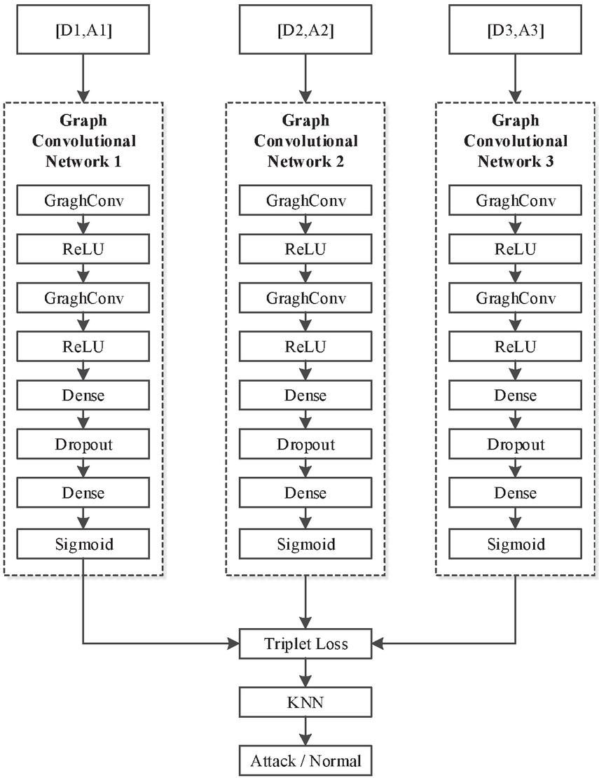
Figure 1 Our proposed tGCN+KNN model.

3.2 Apply tGCN-KNN Method to Intrusion Detection Scenarios Based on Multi-Source Internal State Data of Small Samples

System monitoring data can be used to detect host-based anomalies [33], but it is difficult for a single data source to comprehensively describe the attack, which leading to low detection accuracy. For example, the detection of DoS attack is generally based on the traffic information of a period of history, but DoS attack can also be described by the memory, CPU, network bandwidth and other dimensions of the resource occupation. In addition, the traditional anomaly detection model extracts features separately from the sample data information and ignores the connection between sample entities, which is crucial for the detection of associated threat groups. Multidimensional system state data are considered synthetically in this paper. After transforming the internal state monitoring process and the correlation between processes into graphs, the graph is used as input for anomaly detection. Combined with the attributes of sample data and the correlation information between samples, the GCN framework is used to combine the state information and structural information to make the classification model more accurate.

3.2.1 Data collection

The host to be detected sends the collected status data to the data acquisition server at regular intervals, and these data are stored in the MongoDB database for further analysis and processing. During the acquisition interval, the data acquisition agent is responsible for internal state monitoring of its host and sends the state information to the anomaly detection model in accordance with the specified protocol or format. The internal state send message contains the timestamp, message ID, state type (such as memory state, disk state, port state), and message body. The message body in different state types can contain multiple fields (for example, a memory state message can include the process ID and memory utilization of each process, etc.). The status information is sent in JSON format data. Internal state includes CPU, hard disk, memory state, process state, file state, port state and network state.

State monitoring is implemented by calling various state monitoring Shell commands using Python and reading the results. The common status monitoring Shell commands are shown in Table 1.

Table 1 State detection commands and functions

No.	Shell command	Function
1	top -c -b -n 1 -bw 500	Read the process CPU, memory utilization, and so on
2	Dstat	Reports statistics on kernel threads, virtual memory, disks, traps, and CPU activity.
3	Lsof	Displays a list of all open files and processes.
4	Strace	It is used to track system calls when a process is executing
5	pidstat	It is used to monitor the occupation of CPU, memory, thread, device IO and other system resources of specified processes

The data collection process is implemented in Python, and the Linux shell is interacted with the Popen class of Python subprocess when the shell monitoring command is needed. The data collected by the status monitoring command will be sent to the HTTP server of the master control unit after preprocessing, such as formatting key information. Considering that different monitoring Shell commands often come from different development teams or individuals and thus operate in different data output formats, the purpose of formatting operations is to unify the data format of all commands. Other data preprocessing operations mainly include data summarization. For example, the dstat command will conduct continuous multiple sampling within a collection period, and the data summarization operation will take the average value and variance of the multiple sampling results and then report them to reduce the overall data volume.

The attack information is summarized in Table 2.

Table 2 Attack information

Name	Implementation	Remote/Local
SSH Brute force attack	Hydra command-line tool	Remote
TCP flood attack	tcp flood bin file	Remote
OSPF routing protocol Attack	t50 command-line tool	Remote
Telnet backdoor	Python sniff library	Local
Dirtycow attack	Dirtycow script	Local
Memory and hard disk DoS attack	Python script	Local

3.2.2 Data preprocessing

(1) Digital operation
The data collected from the internal state data include the access files and system calls of the process. These data are text data with semantic characteristics, so they cannot be trained directly. Here, we consider to process these data from the perspective of natural language processing by expressing them into sentences and paragraphs containing semantics. The number of files and system calls is limited and the features can be enumerated, so digitizing this data first reduces the data size. For example, the file name “/usr/local/lib/python3/toSampleData.py” digital after can use two bytes, which greatly reduce the storage space and improve the computational efficiency of subsequent processing.

The idea of digitization is to read the file name or the line number of the system call in the file as the ID, but if the file name or system call is not found in the file, the file name or system call will be put on the last line and its ID will be considered to be the maximum line number.

(2) Feature extraction of sequence of unequal length
For digitized processes, the difficulty of accessing files and system calls is that the sequence of files and system calls accessed by different processes is not long and the length is very different. Equal-length sequences can be used to “fill the zero” for shorter sequences, but this will cause the problem of sparse data to be processed, which will bring great burden to the computational efficiency. The solution is to carry out feature extraction for these different sequences of unequal length, and the data after feature extraction is of equal length. It greatly reduces the data scale and improves the computing efficiency. The extracted feature data can be used in anomaly detection together with other state data.

Feature extraction calls the feature extraction function in Tsfresh library [34], the main function is to input a digital operation after the access file or system call sequence, and then output a fixed number of features.

Tsfresh is a feature engineering tool for processing time series, which can automatically extract more than 100 features from time series. The software package includes several feature extraction methods and a stable feature selection algorithm. TsFresh can automatically calculate a large number of time series features that describe the basic characteristics of time series, such as peak number, average or maximum value, or more complex features such as time reversal symmetry statistics. At the same time, the feature is reduced to the feature that can best explain the trend through hypothesis testing, which is called de-correlation. These feature sets can then be used to construct statistical or machine learning models on time series, often used in regression or classification tasks.

3.2.3 Construction of input matrix F and A

In an intrusion detection scenario based on multi-source internal state data, a process is represented as each node in the graph. Thereinto, the various resource utilization rates of each process, as well as the system calls and features extracted from the accessed files constitute a row in the F matrix. In particular, the entire computer system described by the total resource utilization of CPU, memory, and so on, is represented as node 0, whose resource utilization is the first row of F. L, the number of columns in F, is equal to 60. The rows with less than 60 columns are supplemented by 0, and the overall resource characteristics of the system are represented by N0.

Matrix A represents the relationship between nodes, and the core task of construction is to mine the relationship between processes. In particular, the edge value of node 0 and other nodes is 1, indicating that there is a dependency between the characteristics of total resource utilization of the system and the processes.

The mining method of connecting edges between nodes adopted in this paper is given below:

1. Public files and sockets accessed through the process;

2. Through the call tree of the process;

3. Through the public system call pattern of the process.

For the above three methods, when it is determined that there is a relationship between any two processes, the weight value of the edge between these two processes is increased by one, and the initial value is zero.

3.2.4 Detection process

Offline training steps are as follows:

1 $>$ Detect the status data that need to be analyzed by unit reading, digitize the file data accessed by each process in the status data and the system calls for each process that needs to be monitored.

2 $>$ For the file data visited by each process to be monitored and the system of each process to be monitored, the digitized data is called for feature extraction to solve the problem of uncertain length of data.

3 $>$ Write the data processed in 2 $>$ to a separate table in the database.

4 $>$ The data set is read from the database in 3 $>$ at intervals of T, and a vector sequence is obtained according to the data features of various types of resource utilization, system investigation of active process, access file of active process, etc., and the data set is divided into training set and test set.

5 $>$ After the training data set is transformed into graph G (V,E) data represented by adjacency matrix A and data feature matrix D, the graph structure training data sets of each host are input into their respective graph convolutional neural network model respectively, and the learning is carried out based on multi-source data relations.

6 $>$ The distance feature obtained in step 5 is used as the input of KNN classifier and then trained to obtain the KNN optimal classifier.

The model trained in 6 $>$ was tested with the test data set. The distance features were output through the triple graph neural network and then input to the KNN classifier. Finally, the classification label represented by the graph relationship features was obtained.

7 $>$ Adjust the number of graph convolution layers in the deep learning model. Graph convolution outputs size. The parameters such as the number of neurons in the Dense layer and the network structure were repeated in steps 1 to 6 to obtain a deep learning model with high detection accuracy.

Online detection steps are as follows:

1 $>$ The state data of the master control unit to be predicted is read from the database, and digitize the monitored file data and the system call of each process.

3 $>$ After the training data set is transformed into graph G (V,E) data represented by adjacency matrix A and data feature matrix D, input the trained triple convolution deep learning model finally obtained in the offline training stage to make the prediction.

4 $>$ The distance features obtained in 3 $>$ were input into the KNN classifier trained in the offline stage to obtain the final classification label.

5 $>$ Report the prediction results obtained in 4 $>$ .

The detection process of tGCN-KNN method applied to the intrusion detection scenario based on multi-source internal state data of small samples is shown in Figure 2.

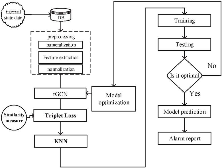
Figure 2 The detection process of tGCN-KNN.

3.3 Apply tGCN-KNN Method to the Intrusion Detection Scenarios Based on Traffic Data of Small Samples

3.3.1 Introduction of traffic datasets

CSE-CIC-IDS2018 Dataset: CSE-CIC-IDS2018 [35] is a dataset mixed with a large number of network traffic and system logs, consisting of 10 days of data, each day of data constitutes a subset of data, with a total size of over 400G. The dataset includes 7 attack types and 16 attack subtypes, including brute force attacks, DoS attacks, surveillance network attacks, and penetration attacks. However, there are few deep learning intrusion detection methods for this dataset [36]. By using the feature generation tool CICFLOWMETER-V3 [37] to analyze the data set of CSE-CIC-IDS2018, about 80 types of feature data can be generated, representing the network traffic and the activity behavior of packets. Table 3 is an overall introduction to the partial data subset of CSE-CIC-IDS2018.

Table 3 Data subset of CSE-CIC-IDS2018

Data Subset	Collection Time	Attack Types	The Total Number of Samples
Sub_DS1	Wednesday-14-02-2018	Positive	663,808
		FTP-BruteForce	193,354
		SSH-Bruteforce	187,589
Sub_DS2	Thursday-15-02-2018	Positive	988,050
		DoS-GoldenEye	41,508
		DoS-Slowloris	10,990
Sub_DS3	Thursday-01-03-2018	Positive	235,778
		Infiltration attack	92,403

UNSW-NB15 Dataset: The Cyber Security Research Group at the Australian Cyber Security Centre (ACSC) built a dataset called UNSW-NB15 [38]. These data is generated in a hybrid manner, using the Ixia Perfect Storm tool (the database that includes CVE) to control the normal and attack behavior of network traffic. A CVE is a database that contains public security vulnerabilities. Two servers are used in the IXIA generator tool, one of which generates normal events and the other generates attack events in the network. Capturing network packets with the TCPdump tool took several hours to generate 100GB of traffic data. Use TCPdump to divide it into approximately 1000MB PACAP files. In LinuxUbuntu14.0.4, Argus and BRO-IDS were used to extract features from the PCAP file. The data can be divided into the following two forms:

(1) Full connection records composed of 2 million connection records;

(2) A partial record of full connection records, consisting of 82,332 training connection records and 175,341 test connection records, which contains 10 types of data. The partial record dataset consists of 42 features and their parallel tags, which are normal and 9 different attacks. The information about the attack categories and their detailed statistics are described in Table 4.

Table 4 UNSW-NB15 dataset

Category	Description	Train	Test
Normal	Normal connection record	56,000	37,000
blur attack	Attacks related to spams, html files penetrations and port scans	18,184	6,062
Analysis	Attacks related to port scan,html file penetrations and spam	2,000	677
Backdoor	Backdoors is a mechanism used to access a computer by evading the background existing security.	1,746	583
DoS	Intruder aims at making network resources down and consequently, resources are inaccessible to authorized users	12,264	4,089
Exploits	The security hole of operating system or the application software is understand by an attacker with the aim to exploit vulnerability	33,393	11,132
Generic	Attacks are related to block-cipher	40,000	18,871
Reconnaissance	Atarget system is observe by an attacker to gather information for vulnerability	10,491	3,496
Shell code	A small part of program termed as payload used in exploitation of software	1,133	378
The worm	Replicate themselves and distributed to other system through the computer network	130	44
Total		93,500	28,481

3.3.2 Construction of input samples F and A

Set a window with the size of W, get all traffic packets in the window to construct A sample data corresponding to F and A matrix. Each node in the graph is represented by source IP $+$ port number, and the number of packets corresponding to each source node $+$ IP is sorted. Then select the first g nodes and consider all subsequent nodes to be the same node. According to experimental tests, the typical value of g is 46. The number of packages for each node contained in a window represents the characteristics of the corresponding node, which means F is a one-dimensional feature. The sample data in each window corresponds to an A matrix. If packets corresponding to two nodes appear successively, the weight of the edge is increased by 1. In addition, if the data corresponding to two nodes is similar, the edge weight will be added to the similarity value. The similarity value is expressed by the cosine distance of the word frequency vector A and B corresponding to the values of two nodes, i.e:

similar = \cos θ = \frac{\sum_{i = 1}^{n} (A_{i} \times B_{i})}{\sqrt{\sum_{i = 1}^{n} {(A_{i})}^{2}} \times \sqrt{\sum_{i = 1}^{n} {(B_{i})}^{2}}}

(4)

Where n represents the length of the word frequency vectors A and B. In this way, a lot of graph structure information is added and the dimension of input data is reduced by the similarity representation of the data, thus improving the computational efficiency.

In addition, the detection procedure is the same as in Section 3.3.2 and will not be described here.

4 Experimental Evaluation

4.1 Evaluation Indicators

In order to evaluate the detection performance of the model, Accuracy, Precision and Recall were selected as evaluation metrics in this paper. The definition of confusion matrix is shown in Table 5, then the definition of other metrics is given.

Table 5 Confusion matrix

True value/Predictive value	Normal data	Abnormal data
Normal data	TN (True Negative)	FN (False Negative)
Abnormal data	FP (False Positive)	TP (True Positive)

Accuracy: The percentage of the number of correctly classified samples relative to the total number of samples.

Accuracy = \frac{T P + T N}{T P + T N + F P + F N}

(5)

Precision: The percentage of the number of samples that are correctly identified as anomalies relative to the number of samples that are identified as anomalies.

Precision = \frac{T P}{T P + F P}

(6)

Recall: The probability that abnormal sample data can be correctly identified.

Recall = \frac{T P}{T P + F N}

(7)

4.2 Experimental Settings

The experimental hardware environment includes: Intel Xeon (Cascade Lake) Platinum 8269 2.5GHz/3.2GHz 4-core CPU, 8GB memory. The proposed tGCN is compared with tCNN and CNN, which have good performance, on public network datasets CSE-CIC-IDS2018 and UNSW-NB15 and internal state datasets collected by ourselves. The structure and parameters of all deep learning models are optimized for fair comparison.

Table 6 The relationship between model detection accuracy and the number of training samples

		Accuracy of Different Number of Samples

Dataset	Model	10	20	30	40	50
CSE-CIC-IDS2018	tGCN	93.7%	94.8%	95.3%	95.8%	96.3%
CSE-CIC-IDS2018	tCNN	65.1%	68.1%	75.7%	81.3%	88.6%
UNSW-NB15	tGCN	92.9%	93.2%	94.4%	95.0%	95.5%
UNSW-NB15	tCNN	63.7%	66.2%	74.3%	80.9%	87.8%
Internal state dataset	tGCN	92.8%	94.6%	95.5%	95.9%	96.6%
Internal state dataset	tCNN	62.2%	63.4%	71.9%	78.3%	87.8%

4.3 Experimental Comparison

First of all, when the number of training samples is small, as the training samples change from 10 to 50, the accuracies of the two metric learning models tGCN and tCNN on the three data sets are compared (as shown in Table 6, where Acc-s represents the accuracy when the number of training samples is s). In order to conduct a comprehensive test, the number of positive and negative samples to be tested is 1000. Average the results of 50 repeated experiments to get the final results. It can be seen from the table that when the number of samples is very small, the accuracy of the tGCN model proposed in this article is still very high, but the accuracy of the tCNN model is poor. As the number of samples gradually increases, the accuracy of tCNN increases rapidly, while the accuracy of tGCN models slowly increases, and tCNN begins to approach tGCN. But tGCN has always outperformed tCNN. Compared with tCNN, tGCN improves accuracy by 49.2%. The reason is that tGCN uses graph structure data to make up for a large amount of information lost in Euclidean structure data.

Table 7 shows the performance comparison of Accuracy, Precision and Recall of the three models on different data sets when the number of samples participating in the training is 150. It can be seen from the table that the Accuracy, Precision and Recall of tGCN are all higher than the other two methods in the three datasets. Compared with tCNN and CNN, the Accuracy of tGCN is improved by 7.1% and 15.5% respectively in the CSE-CIC-IDS2018 dataset. In the other two datasets, tGCN also shows great advantages in Accuracy, Precision and Recall. The reason is that tGCN can utilize the advantages of graph neural network and metric learning method to maximize its advantages in small sample detection scenarios.

Table 7 Performance comparison of three models with fixed number of training samples

	Accuracy (%)			Precision (%)			Recall (%)

	tGCN	tCNN	CNN	tGCN	tCNN	CNN	tGCN	tCNN	CNN
CSE-CIC-IDS2018	99.3	92.7	86.0	98.7	93.2	85.5	100.0	92.0	86.7
UNSW-NB15	98.0	91.3	84.7	98.6	90.8	83.3	97.3	92.0	86.7
Internal state dataset	98.7	92.0	86.0	98.7	90.9	86.5	98.7	93.3	85.3

Table 8 Performance comparison of the three models when the test data class contains some new attack classes

	Accuracy (%)			Precision (%)			Recall (%)

	tGCN	tCNN	CNN	tGCN	tCNN	CNN	tGCN	tCNN	CNN
CSE-CIC-IDS2018	98.0	88.7	80.6	97.4	89.2	80.2	98.7	88.0	81.3
UNSW-NB15	96.7	87.3	81.3	96.0	86.8	81.3	97.3	88.0	81.3
Internal state dataset	97.3	90.0	79.3	97.3	90.5	78.9	97.3	89.3	80.0

Table 8 shows the performance comparison of Accuracy, Precision and Recall of the three models on different data sets when the number of samples participating in the training is 150 and some new attack classes are included in the test data class. It can be seen from the table that the Accuracy, Precision and Recall of tGCN in the three datasets are all higher than the other two methods. Compared with tCNN and CNN, the Accuracy of tGCN is improved by 10.5% and 21.6% respectively in the CSE-CIC-IDS2018 dataset. In the other two datasets, tGCN also shows great advantages in Accuracy, Precision and Recall. By comparing Tables 7 and 8, it can be seen that tGCN has a more prominent advantage in detecting new attack classes than the other two methods. The main reason may be that the graph convolutional network extracts the main key information, so as to ensure the obvious distinction between anchor samples and attack samples to be detected.

Table 9 shows the performance comparison of Accuracy, Precision and Recall of the three models on different data sets when the number of samples participating in the training is 150 and random perturbation is added to the test data. It can be seen from the table that the Accuracy, Precision and Recall of tGCN in the three data sets are all higher than the other two methods. Compared with tCNN and CNN, the Accuracy of tGCN is improved by 21.9% and 28.4% respectively in the CSE-CIC-IDS2018 dataset. In the other two datasets, tGCN also shows great advantages in Accuracy, Precision and Recall. By comparing Table 7 with Table 9, it can be seen that tGCN has a more prominent advantage in dealing with random disturbances, namely robustness, than the other two methods. The main reason is that the random disturbance in the graph convolutional network is only affected by the similarity measure between the valid data packets corresponding to the two nodes in the A matrix, while such disturbance will not have much change on the similarity measure and has no effect on other data information in the input sample. The other two methods are mainly based on the data subject to random disturbance, which will have a great impact on the detection results.

Table 9 Performance comparison of three models with random disturbance

	Accuracy (%)			Precision (%)			Recall (%)

	tGCN	tCNN	CNN	tGCN	tCNN	CNN	tGCN	tCNN	CNN
CSE-CIC-IDS2018	96.7	79.3	75.3	97.2	79.7	75.0	96.0	78.6	76.0
UNSW-NB15	95.3	78.7	74.6	95.9	77.9	74.0	94.7	80.0	76.0
Internal state dataset	96.0	79.3	77.3	94.8	78.9	77.3	97.3	80.0	77.3

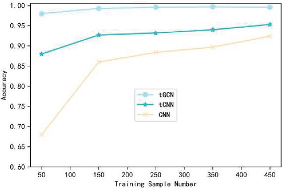
Figure 3 Comparison of the influence of training sample data on the accuracy of CSE-CIC-IDS2018 data set.

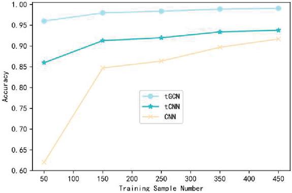
Figure 4 Comparison of the influence of training sample data on the accuracy of UNSW-NB15 data set.

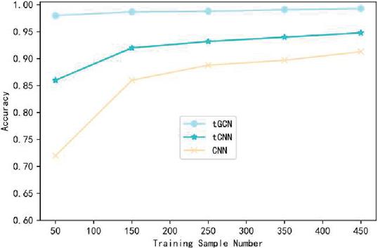
Figure 5 Comparison of the influence of training sample data on the accuracy of host state data set.

Figures 3–5 respectively shows the variation curve of Accuracy of the three methods with the number of training samples on the three datasets. It can be seen that the Accuracy of the three methods is gradually improved with the increasing number of samples participating in the training. However, when the number of samples participating in training is small, the advantage of tGCN method is more obvious. When the number of samples participating in the training is 50, compared with tCNN and CNN methods, the Accuracy of tGCN method is respectively improved by 11.4% and 58.1% in the CSE-CIC-IDS2018 dataset. Similar results were obtained on the other two datasets. This indicates that tGCN has a more prominent advantage in small sample scenarios. It also shows that the advantage of triple metric learning using small sample intrusion detection scenarios is obviously better than the traditional deep learning models such as CNN. Combined with metric learning and graph convolutional neural network, the proposed method maximizes its advantages in small sample scenarios. With the increase of the number of trainable samples, the advantage of tGCN method over other methods is gradually weakened, and the Accuracy of tCNN and CNN method is constantly close to that of tGCN.

Figure 6 compares the normalized training time of the three comparison methods. In the three datasets, the normalized training time of tGCN is much smaller than that of the other two models. Compared with tCNN and CNN models, tGCN shortens the training time by 88.6% and 81.9% respectively. tGCN also has a great advantage in training time because the GCN data structure modeled in this paper greatly compresses the dimensions of the data while retaining the information of the key graph structure.

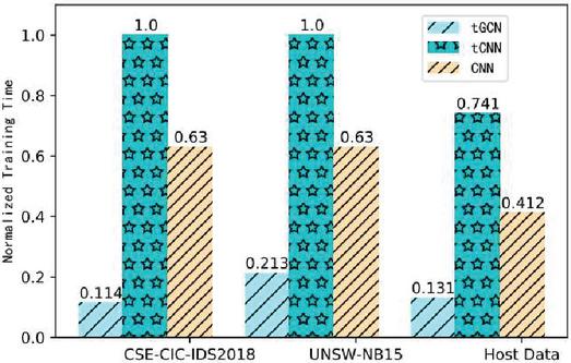
Figure 6 Comparison of normalized training time of three models.

5 Conclusion

In the face of new unknown threats that may appear in the future in the field of network security, an innovative method of network intrusion detection based on triples of small samples graph neural network is proposed, which provides an effective means to detect abnormal cases with only a small amount of sample data. By modeling the traffic data and internal state data as graph data structure, the data dimension is reduced and the computational efficiency is improved. The innovation point is that the trigram sample data is input into the trigram convolutional neural network, in which the trigram convolutional neural network shares the network structure and parameters as the distance feature extraction network, and the three-element loss is responsible for the training network, so that the distance between two similar samples is far less than the distance between different samples. Finally, a simple and efficient KNN algorithm is used to further classify the distance features. TGCN-KNN proposed in this paper can effectively classify abnormal data and normal data, and achieves the expected effect in small sample experimental scenarios constructed by reference stream datasets CSE-CIC-IDS2018, UNSW-NB15 and internal state datasets. In addition, the results of the three methods were compared when the sample size was sufficient. Even in the case of adding random interference, TGCN-KNN still has great advantages.

Acknowledgements

Funding Statement: This work was sponsored by the National Key Research and Development Program of China (Grants 2018YFB0804002 and 2017YFB0803204).

Conflicts of Interest: The authors declare that they have no conflicts of interest to report regarding the present study.

References

[1] T. Hamed, R. Dara, and S. C. Kremer, “Network intrusion detectionsystem based on recursive feature addition and bigram technique,” Computers & Security, vol. 73, pp. 137–155, 2018.

[2] Y. LeCun, Y. Bengio and G. Hinton, “Deep learning,” Nature, vol. 521, pp. 436–444, 2015.

[3] W. Wang, Y. Sheng, J. Wang, X. Zeng, X. Ye et al., “HAST-IDS: Learning hierarchical spatial-temporal features using deep neural networks to improve intrusion detection,” IEEE Access, vol. 6, pp. 1792–1806, 2018.

[4] E. Min, J. Long, Q. Liu, J. Cui, and W. Chen, “TR-IDS: Anomalybased intrusion detection through text-convolutional neural network andrandom forest,” Security and Communication Networks, vol. 2018, Article ID. 4943509, 2018.

[5] L. Bilge and T. Dumitraş, “Before we knew it: an empirical study of zero-day attacks in the real world,” in Proceedings of the 2012 ACM Conference on Computer and Communications Security, Raleigh North Carolina, USA, pp. 833–844, 2012.

[6] K. Zhao, X. Jin and Y. Wang, “Survey on few-shot learning,” Journal of Software, pp. 225–236, 2020.

[7] Santoro, S. Bartunov, M. Botvinick, D. Wierstra, and T. Lillicrap, “Meta-learning with memory-augmented neural networks,” in Proceedings of the 33rd International Conference on International Conference on Machine Learning, New York, USA, vol. 48, pp. 1842–1850, 2016.

[8] Vinyals, C. Blundell, T. Lillicrap, K. Kavukcuoglu and D. Wierstra, “Matching networks for one shot learning,” in Proceedings of the 30th International Conference on Neural Information Processing Systems, Barcelona, Spain, pp. 3630–3638, 2016.

[9] J. Snell, K. Swersky, and R. Zemel, “Prototypical networks for few-shotlearning,” in NIPS 2017 Proceedings, Long Beach, CA, USA, pp. 4077–4087, 2017.

[10] F. Sung, Y. Yang, L. Zhang, T. Xiang, P. H. Torr et al., “Learning to compare: Relation network for few-shot learning,” in Proc. IEEE/CVF Conference on Computer Vision and Pattern Recognition, Salt Lake City, UT, USA, pp. 1199–1208, 2018.

[11] R. Zhang, T. Che, Z. Ghahramani, Y. Bengio, and Y. Song, “MetaGAN: An adversarial approach to few-shot learning,” in Proceedings of the 32nd International Conference on Neural Information Processing Systems, Montreal, Canada, pp. 2365–2374, 2018.

[12] S. Gurung, M. K. Ghose and A. Subedi, “Deep learning approach on network intrusion detection system using NSL-KDD dataset,” International Journal of Computer Network and Information Security(IJCNIS), vol. 11, no. 3, pp. 8–14, 2019.

[13] M. M. Hassan, A. Gumaei, A. Alsanad, M. Alrubaian, “A hybrid deep learning model for efficient intrusion detection in big data environment,” Information Sciences, vol. 513, pp. 386–396, 2020.

[14] M. Liu, Z. Xue, X. Xu, C. Zhong and J. Chen, “Host-based intrusion detection system with system calls: Review and future trends,” ACM Computing Surveys, vol. 51, no. 5, pp. Article No. 98, 2018.

[15] Z. Zhang, P. Cui and W. Zhu, “Deep learning on graphs: A survey,” IEEE Transactions on Knowledge and Data Engineering, 2020.

[16] N. Shone, T. N. Ngoc, V. D. Phai and Q. Shi, “A deep learning approach to network intrusion detection,” IEEE Transactions on Emerging Topics in Computational Intelligence, vol. 2, no. 1, pp. 41–50, 2018.

[17] J. R. Reuning, “Applying term weight techniques to event log analysis for intrusion detection,” Masters Paper, University of North Carolina at Chapel Hill, USA, 2004.

[18] F. Apap, A. Honig, S. Hershkop, E. Eskin and S. Stolfo, “Detecting malicious software by monitoring anomalous windows registry accesses,” in Wespi A., Vigna G., Deri L. (eds) Recent Advances in Intrusion Detection. RAID 2002. Lecture Notes in Computer Science, vol. 2516. Springer, Berlin, Heidelberg, pp. 36–53, 2002.

[19] Ou, “Host-based intrusion detection systems inspired by machine learning of agent-based artificial immune systems,” in 2019 IEEE International Symposium on INnovations in Intelligent SysTems and Applications (INISTA), Sofia, Bulgaria, pp. 1–5, 2019.

[20] Santoro, S. Bartunov, M. Botvinick, D. Wierstra and T. Lillicrap, “One-shot Learning with Memory-Augmented Neural Networks,” in Proceedings of the 33rd International Conference on International Conference on Machine Learning, New York, USA, pp. 1842–1850, 2016.

[21] T. Munkhdalai and H. Yu, “Meta networks,” in Proceedings of the 34th International Conference on Machine Learning, Sydney, Australia, pp. 2554–2563, 2017.

[22] J. Howard J and S. Ruder, “Universal Language Model Fine-tuning for Text Classification,” in Proceedings of the 56th Annual Meeting of the Association for Computational Linguistics (Volume 1: Long Papers), Melbourne, Australia, pp. 328–339, 2018.

[23] Nakamura and T. Harada, “Revisiting fine-tuning for few-shot learning,” ICLR 2020 Conference Withdrawn Submission.A. Nakamura, T. Harada, “Revisiting fine-tuning for few-shot learning,” arXiv preprint arXiv: 1910.00216, 2019.

[24] G. Koch, R. Zemel and R. Salakhutdinov, “Siamese neural networks for one-shot image recognition,” in ICML deep learning workshop, vol. 2, 2015.

[25] Vinyals, C. Blundell, T. Lillicrap, K. Kavukcuoglu and D. Wierstra, “Matching networks for one shot learning,” in Proceedings of the 30th International Conference on Neural Information Processing Systems, Barcelona, Spain, pp. 3630–3638, 2016.

[26] L. B. Jiang, X. L. Zhou, F. W. Jiang and L. Che, “One-shot learning based on improved matching network,” Systems Engineering and Electronics, vol. 41, no. 6, pp. 1210–1217, 2019.

[27] V. G. Satorras and J. B. Estrach, “Few-shot learning with graph neural networks,” in Proc. ICLR, Vancouver, Canada, 2018.

[28] J. Kim, T. Kim, S. Kim and C. D. Yoo, “Edge-labeling graph neural network for few-shot learning,” in Proceedings of the IEEE Conference on Computer Vision and Pattern Recognition, Long Beach, CA, USA, pp. 11–20, 2019.

[29] S. Gidaris and N. Komodakis, “Generating Classification Weights with GNN Denoising Autoencoders for Few-Shot Learning,” in 2019 IEEE/CVF Conference on Computer Vision and Pattern Recognition (CVPR), Long Beach, CA, USA, pp. 21–30, 2019.

[30] J. Jiang, J. Chen, T. Gu, K. K. R. Choo, C. Liu et al., “Anomaly detection with graph convolutional networks for insider threat and fraud detection,” in MILCOM 20+19–2019 IEEE Military Communications Conference (MILCOM), Norfolk, VA, USA, pp. 109–114, 2019.

[31] E. Hoffer and N. Ailon, “Deep metric learning using triplet network,” in Feragen A., Pelillo M., Loog M. (eds) Similarity-Based Pattern Recognition. SIMBAD 2015. Lecture Notes in Computer Science, vol 9370. Springer, Cham, pp. 84–92, 2015.

[32] V. P. Kshirsagar, M. R. Baviskar and M. E. Gaikwad, “Face recognition using Eigenfaces,” in Proc. 2011 3rd International Conference on Computer Research and Development, Shanghai, China, pp. 302–306, 2011.

[33] M. Liu, Z. Xue, X. Xu, C. Zhong and J. Chen, “Host-based intrusion detection system with system calls: review and future trends,” ACM Computing Surveys (CSUR), vol. 51, no. 5, Article No. 98, 2018.

[34] M. Christ, N. Braun, J. Neuffer and A. W. Kempa-Liehr, “Time series Feature extraction on basis of scalable hypothesis tests (tsfresh – A Python package),” Neurocomputing, vol. 307, pp. 72–77, 2018.

[35] J. Kim, Y. Shin and E. Choi, “An intrusion detection model based on a convolutional neural network,” Journal of Multimedia Information System, vol. 6, no. 4, pp. 165–172, 2019.

[36] CSE-CIC-IDS2018 on AWS, https://www.unb.ca/cic/datasets/ids-2018.html

[37] CICFlowMeter, https://www.unb.ca/cic/research/applications.html#CICFlowMeter

[38] N. Moustafa and J. Slay, “UNSW-NB15: a comprehensive data set for network intrusion detection systems (UNSW-NB15 network data set),” in Proc. 2015 Military Communications and Information Systems Conference (MilCIS), Canberra, ACT, pp. 1–6, 2015.

Biography

Yue Wang received the bachelor’s degree from the School of Computer Science, Sichuan University, Chengdu, China, in 2018. She is currently pursuing the master’s degree with PLA Information University, Zhengzhou, China. Her research interests include new network architectures for the next generation Internet and network security.

Yiming Jiang received the Ph.D. degree from PLA Information University, Zhengzhou, China in 2014. Currently, he is an assistant researcher in PLA Information University. His research interests include new network architectures for the next generation Internet, network security and cloud computing.

Julong Lan is a professor and chief engineer in PLA Information University. His research interests include new network architectures for the next generation Internet and network security.