Effective Algorithm to Control Depth Level for Performance Improvement of Sound Tracing

Eunjae Kim¹, Juwon Yun¹, Woonam Chung¹, Jae-Ho Nah², Youngsik Kim³, Cheoung Ghil Kim⁴ and Woo-Chan Park^1,*

¹Sejong University, Seoul, South Korea
²Sangmyung University, Seoul, South Korea
³Korea Polytechnic University, South Korea
⁴Namseoul University, Korea
E-mail: ejkim@rayman.sejong.ac.kr; juwon@rayman.sejong.ac.kr; hobit37@gmail.com; nahjaeho@gmail.com; kys@kpu.ac.kr; cgkim@nsu.ac.kr; pwchan@sejong.ac.kr
$^{*}$ Corresponding Author

Received 28 April 2021; Accepted 09 December 2021; Publication 19 February 2022

Abstract

Sound tracing, a 3D sound rendering technology based on ray tracing, is a very costly method for calculating sound propagation. To reduce its expense, we propose an algorithm for adjusting the depth based on frame coherence and spatial characteristics. The results of the experiment indicate that when the sound source and listener were indoors, the reflection path loss rate was 3%, the diffraction path loss rate was 15.4%, and the total frame rate increased by 6.25%. When the listener was outdoors and the sound source was indoors, the reflection path and diffraction path loss rate were 0%, and the total frame rate was increased by 33.33 compared to the conventional method. Thus, the proposed algorithm can improve rendering performance while minimizing path loss rate.

Keywords: Sound tracing, sound rendering, sound propagation, ray tracing, virtual reality.

1 Introduction

Based on 3D geometric models, sound tracing simulates audio that changes in real-time depending on the location of objects, materials, listeners, and sound sources in virtual space. In addition, the technology provides the user with an aural sense of space by reproducing physical characteristics of sound such as reflection, transmission, diffraction, and absorption [1, 2].

However, simulating physically-based sound with surrounding objects and materials in real-time requires a large computational expense and high power consumption [3]. Therefore, there is a limit to real-time processing of sound tracing in a resource-limited environment such as a mobile device. For this reason, it is essential to reduce power consumption and calculation cost to provide an auditory immersion across a range of platforms.

In this paper, we propose an algorithm that will solve the problem of the computational cost of real-time sound tracing. The algorithm adjusts the maximum depth of a ray for the sound propagation using spatial and frame coherence characteristics. As a result, this method can reduce the amount of computation needed for sound propagation and improve performance through depth adjustment.

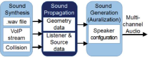
Figure 1 Sound tracing steps.

2 Background

2.1 Sound Tracing

Sound tracing is a 3D sound rendering technology that combines sound processing and ray tracing technology. Figure 1 shows the three processing steps of sound tracing, whereby sound synthesis creates sound effects based on user interaction, sound propagation simulates the process of transmitting the synthesized sound to the listener, and sound generation (auralization) takes the dry-audio generated in the first step and the impulse response (IR) calculated in the second and convolutes them to generate the final sound, which it outputs to the user’s final output device. Of these three steps, sound propagation is the most expensive to calculate and very difficult to process in real-time. That is, in order to process sound rendering in real-time, it is essential to accelerate the sound propagation.

2.2 Sound Propagation

Sound propagation algorithms are largely classified as either wave-based numerical methods or geometric acoustic(GA) methods. Wave-based numerical methods calculate the propagation path by taking into account the waveform as real-word sound processing [4, 5, 6, 7, 8]. Since this method performs numerical calculation numerically by applying the relationship between the sound source and the listener in the wave equation for the surrounding environment, it is possible to compute an accurate propagation path, although the cost of this calculation is high.

GA methods trace the propagation path of sound using a single ray, frusta or beam. The physical properties of sound are simulated through sound propagation, and calculated in real-time. Therefore, GA methods are suitable for dynamic scenes that require real-time processing.

M. Taylor et al. [10] parallelized sound reflection processing using GPU-based ray-tracing applied by a multi-view tracking algorithm so that early specular reflection and first-order diffraction were accelerated through GPU parallelism. C. Schissler et al. [12] introduced a method of repeatedly calculating diffuse reflection by combining radiosity and path tracing. In this method, reflection and diffraction paths are calculated using GA, and statistical techniques are used for dynamic scenes.

C. Schissler et al. [11] used sphere-sound sources unlike the point-sound sources of [9], and performed backward-ray tracing based on the listener. In addition, sub-linear scaling was achieved by clustering sound sources far from the listener. C. Cao et al. [13] used a bidirectional path tracing method using multiple importance sampling.

3 Analysis of Sound Propagation Characteristics

3.1 Rays Characteristics According to Space

Sound propagation processing is performed using guide and source rays. A guide ray is created from a listener, and a source ray is created from a sound source. Traversal and collision-detection are performed between the ray and triangles. The ray hit by the triangles generates another reflected ray, and each of these reflections is refers to depth. The sound propagation recursively performs this process until the depth reaches max-depth. When sound propagation is performed in this way, the triangles hit by the guide ray provide the basis for early reflection, and those hit by the source ray provide the basis for late reverberation. Sound propagation can grasp a scene’s characteristics through the guide ray and source ray.

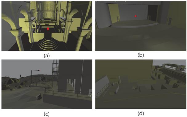
Figure 2 (a): Sibenik(indoor) – 75k triangles, (b): Concert hall (indoor) -– 24k triangles, (c): Bootcamp (complex) – 130k triangles, (d): Angrybot (complex) – 38k triangles.

Table 1 Average guide ray count per each depth

Scene	Depth1	Depth2	Depth3	Depth4
Sibenik (Indoor)	1024	1023	1023	1020
Concerthall (Indoor)	1024	1024	1024	1024
Bootcamp (Outdoor)	1024	428	69	26
Angrybot (Complex)	1024	773	523	365

To check the characteristics of a scene through the guide ray across various environments, experiments were performed in 4 scenes as shown in Figure 2. Sibenik and Concert hall were an indoor scenes, Bootcamp was an outdoor scene, and Angrybot was a complex scene with indoor and outdoor characteristics. Table 1 shows the number of guide rays for each depth across 4 scenes. In the sound propagation system, the number of guide rays was set to 1,024, max-depth was set to 4,and the average value for each depth was measured for 10 frames. The results of the experiment showed that the indoor scene maintained the number of guide rays for all depths. As the depth increased outdoors, the number of guide rays decreased. The complex scene showed that the number of guide rays decreased as the depth increased, but the number was lower than that of the outdoor scene.

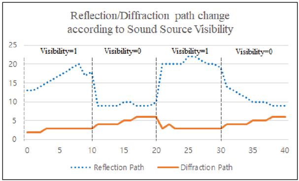
Figure 3 Change of the number of reflection/diffraction paths per frames.

3.2 Reflection/Diffraction Path Count According to Sound Source Visibility

The number of valid reflections and diffraction paths varies depending on the visibility of the sound source. The valid path is a path from the sound source to the listener and affects making final audio. The sound source visibility is whether there is a direct path from the listener to the sound source.

Figure 3 shows the change in the number of valid reflection- and diffraction-paths according to a sound source visibility. In the figure, the x-axis represents the frame number and the y-axis represents the number of paths. If the sound source has a direct path, its visibility is one; otherwise, it is zero.

The experiment was performed in the Angrybot complex scene and the number of valid reflection and diffraction paths was measured for 40 frames while moving the listener from the visible areas to the invisible areas. The results of experiment show that the reflection path tended to increase when the sound source visibility was one and decrease when it was zero. On the other hand, the diffraction path tended to increase slightly when visibility was 0. Through this, it can be seen that sound source visibility had a large influence on the number of valid paths.

3.3 Frame Coherence

According to our experiments, the sound propagation showed high frame coherence. Table 2 shows the probability that a valid frame is the same in the current and previous frames for each depth while performing sound tracing for 100 frames in the Bootcamp scene. The valid frame represents a frame in which the valid paths exist. If the valid paths exist in both the previous and current frames at all depths, it can be said that the valid frame is the same at all depths. This means that the frame coherence is high.

Table 2 Probability that the current valid frame equals the previous valid frame for 100 frames

Scene	Depth1	Depth2	Depth3
Bootcamp(Indoor)	70.71%	90.91%	86.87%
Bootcamp(Outdoor)	96.97%	100.00%	100.00%

The result of experiment show that the indoor scene had a higher probability of having the same valid frame as the depth increased. On the other hand, outdoor scenes had a high probability of having the valid frame with the previous frame at all depths. This means that there is a high probability that the valid frames between frames are the same regardless of the scene’s characteristics. As a result, we can predict whether the next frame is valid or not by determining the validity of the current frame for each depth.

4 Proposed Algorithm

4.1 Proposed Sound Propagation Flow-chart

In this section, we will first describe the entire sound propagation flow and then outline the proposed adaptive depth control(ADC) algorithm in detail.

Figure 4 shows the proposed sound propagation flow-chart with steps consisting of SetupProcessing, RayGeneration, Traversal&Intersection Test (TnI), HitPointCalc, Propagation Path Validation& Reverb Geometry Collector (PPVnRGC), and PathReverbIRCalc.

The SetupProcessing step manages the sound propagation mode, generates ray information according to the mode, and delivers it to the RayGeneration step. The proposed depth control algorithm is also performed in this step. The RayGeneration step creates a ray using the information received in the previous step and delivers the ray data to the TnI step. In the TnI step, the generated ray traverses through the acceleration structure and performs collision-detection between the ray and triangles. The HitPointCalc step calculates the hit point.

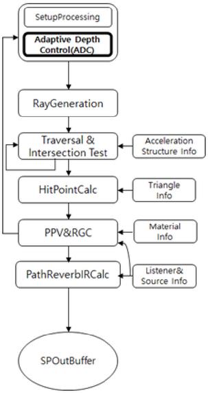
Figure 4 Proposed sound propagation flow chart.

The PPVnRGC step executes either Propagation Path Validator (PPV) or Reverb Geometry Collector (RGC) depending on the characteristics of the ray. The PPV step checks whether the path is valid based on the information calculated in the previous step and the location information of the listener and sound source. In the RGC step, information necessary for reverb is stored in a buffer using a source ray. Finally, the PathReverbIRCalc creates Impulse Response (IR) data using the information received through PPVnRGC and stores the generated data in the SPOutBuffer.

The ADC algorithm proposed in this paper uses sound propagation characteristics according to spatial and temporal coherence. The factor using the temporal coherence characteristic adjusts the depth using the average value of valid frames of previous frames. The ADC for depth control was added to the Setup Processing step. If the appropriate ray depth can be adjusted according to the situation, the quality of sound propagation will be minimized while the amount of computing is reduced, and the performance will be improved as the amount of calculation is reduced.

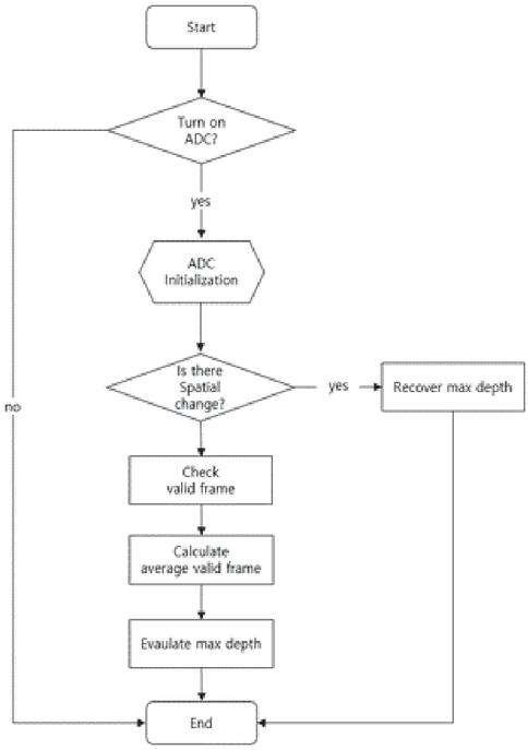
Figure 5 Proposed algorithm flow chart.

4.2 Adaptive Depth Control Algorithm

Figure 5 shows the proposed algorithm flow-chart. First, the algorithm checks whether the ADC is activated. When this is activated, variables are initialized and the ADC is performed. The next step checks whether there is a spatial change of a sound source or listener calculated in the previous frame. The spatial change of sound source or listener is calculated as follows:

$S (I, F) = V (I) \| ((P (G) \| P (I, R)) \hat{} S (I, F - 1))$	(1)
$P (G) = [\frac{GuidePlaneCount}{GuideRayCount}]$	(2)
$P (I, R) = [\frac{{SourcePlaneCount}_{(I)}}{{GuideRayCount}_{(I)}}]$	(3)

In Equation (1), $S (I, F)$ denotes the presence or absence of a change in the spatial position of the sound source in the frame. I and F denote the ID of the sound source and frame number, respectively. If $S (I, F)$ is one, there is a spatial change, and if $S (I, F)$ is zero, there is no spatial change.

$V (I)$ represents visibility between the sound source and the listener. If $V (I)$ is one, there is a direct path between the sound source and the listener in the frame. If $S (I, F)$ is zero, there is no direct path between the sound source and the listener in the frame.

In Equation (2), $P (G)$ represents the result of rounding after dividing the guide plane count by the guide ray count. In total, 1024 guide rays are shot from each listener. The guide plane is a plane (or triangle) that is hit by the guide ray. If $P (G)$ is one, the listener is in a space with a high possibility of reflection. If $P (G)$ is zero, the listener is in a space with less possibility of reflection.

In Equation (3), $P (I, R)$ is the result of rounding the result by dividing the source plane count by the source ray count. In total, 128 source rays are shot from each source. The source plane is a plane that is hit by the source ray. If $P (I, R)$ is one, the sound source is in a space where there is ample reflection. If $P (I, R)$ is zero, the sound source is in a space with poor reflection.

As a result, when the visibility between the listener and the sound source changes when the current frame is compared with the previous frame, or when the sound source and the listener change space, $S (I, F)$ becomes one. At this time, the depth is recovered to four, which is the max-depth that can be generated in sound propagation.

If there is no spatial change, the new depth is calculated based on the valid frames for each depth. The ADC stores valid frame values for each depth for the previous 20 frames while performing sound tracing. If the current frame is the 30th frame and there is no spatial change, the ADC calculates the average value of the valid frame for each depth for the previous 20 frames (10 $\sim$ 29 frames) and divides it by 20. For each depth, a depth with a result value greater than 0.5 is found, and the largest depth among them is determined to be the new depth.

Table 3 The result of applying ADC

Frame Number	R0	R1	R2	R3	D0	D1	D2	D3	Path Loss Rate (R/D) (%)	Frame Rate (ms)
50th frame	ADC	12	4	9	7	6	3	2	0	3.03 /15.4	15
	Non-ADC	13	4	9	7	6	3	3	1		16
	Difference	1	0	0	0	0	0	1	1		1
500th frame	ADC	8	2	7	7	5	3	1	0	7.69 / 0	12
	Non-ADC	8	3	7	8	5	3	1	0		13
	Difference	0	1	0	1	0	0	0	0		1
1000th frame	ADC	0	0	0	0	1	0	0	0	0 / 0	6
	Non-ADC	0	0	0	0	1	0	0	0		9
	Difference	0	0	0	0	0	0	0	0		3
R-Number: the R is the reflection path count, *D-Number: the D is the diffraction path count, the number is order.

5 Experiment Results

In this paper, we experimented in the Bootcamp environment, which is an environment with complex spaces that are meaningful in ADC experiments. For a range of experimental conditions, one sound source was placed indoors, and the listener performed an experiment while moving between indoors and outdoors.

Table 3 shows the results of experiment at the 50th, 500th, and 1000th frames when applying depth control to the Bootcamp environment. The factors of the results are the number of valid paths, path loss rate, and frame rate for each reflection depth (R) and diffraction (D) in a frame in which the sound source and listener are in different space.

In the 50th frame, both the sound source and the listener were located indoors. The loss rate of the reflection path was 3.03%; the loss rate of the diffraction path was 15.4%; and the frame rate when using ADC was 6.25% better than when ADC was not utilized.

In the 500th frame, the sound source was located indoors, and the listener was located in an ambiguous place—neither indoors nor outdoors. The loss rate of the reflection path was 7.69%, the loss rate of the diffraction path was 0%, and the frame rate when ADC was employed was 7.69% better than when the ADC was not employed.

In the 1000th frame, the sound source was located indoors, and the listener was located outdoors. The loss rate of the reflection path was 0%, the loss rate of the diffraction path was 0%, and the frame rate when using ADC was 33.33% better than when the ADC was not utilized.

6 Conclusion

In this paper, we proposed an ADC method to improve the performance of sound tracing. For ADC, spatial characteristics and frame coherence characteristics were employed.

To adjust the depth, the average number of valid frames of the previous frames for each depth was applied. In addition, to obtaining the timing to recover the depth, the timing to recover the depth was gathered using the visibility of the sound source, guide plane ratio, and reverb plane ratio.

The ADC experiment with the proposed method reveals that, in the case of path loss rate, when the listener was inside, the reflection path loss rate was 3.03% and the diffraction path loss rate was 15.4%. When the listener was outside, the reflection and diffraction path loss rate showed a loss rate of 0%.

In terms of performance, when the listener was indoors, the frame rate increased by 6.25%, and when the listener was outdoors, the frame rate increased by 33.3%. These findings confirm that the proposed ADC method can minimize potential path loss and improve frame rates.

Acknowledgement

This material is based upon work supported by the Ministry of Trade, Industry & Energy(MOTIE, Korea) under Industrial Technology Innovation Program (20010072).

References

[1] M. Vorlander, Auralization: Fundamentals of Acoustics, Modelling Simulation, Algorithms and Acoustic Virtual Reality, Springer, 2008.

[2] Funkhouser, Thomas, Nicolas Tsingos, and Jean-Marc Jot, Survey of methods for modeling sound propagation in interactive virtual environment systems, Presence and Teleoperation, 2003.

[3] Hong., T. H. Joo, and W.-C. Park., Real-time sound propagation hardware accelerator for immersive virtual reality 3D audio, Proceedings of the 21st ACM SIGGRAPH Symposium on Interactive 3D Graphics and Games, 2017.

[4] Raghuvanshi, Nikunj and Narain, Rahul and Lin, Ming C, Efficient and accurate sound propagation using adaptive rectangular decomposition, IEEE Transactions on Visualization and Computer Graphics, 15(5):789–801, 2009.

[5] Raghuvanshi, Nikunj and Snyder, John and Mehra, Ravish and Lin, Ming and Govindaraju, Naga, Precomputed wave simulation for real-time sound propagation of dynamic sources in complex scenes, ACM SIGGRAPH, 1–11, 2010.

[6] Mehra, Ravish and Raghuvanshi, Nikunj and Antani, Lakulish and Chandak, Anish and Curtis, Sean and Manocha, Dinesh, Wave-based sound propagation in large open scenes using an equivalent source formulation, ACM Transactions on Graphics (TOG), 32(2):1–13, 2013.

[7] Mehra, Ravish and Raghuvanshi, Nikunj and Chandak, Anish and Albert, Donald G and Keith Wilson, D and Manocha, Dinesh, Acoustic pulse propagation in an urban environment using a three-dimensional numerical simulation, The Journal of the Acoustical Society of America, 135(6):3231–3242, 2014.

[8] Mehra, Ravish and Rungta, Atul and Golas, Abhinav and Lin, Ming and Manocha, Dinesh, Wave: Interactive wave-based sound propagation for virtual environments, IEEE transactions on visualization and computer graphics, 21(4):434–442, 2015.

[9] Taylor, Micah and Chandak, Anish and Mo, Qi and Lauterbach, Christian and Schissler, Carl and Manocha Dinesh, i-sound: Interactive gpu-based sound auralization in dynamic scenes, Tech. Rep. TR10-006, 2010.

[10] Taylor, Micah and Chandak, Anish and Mo, Qi and Lauterbach, Christian and Schissler, Carl and Manocha, Dinesh, Guided multiview ray tracing for fast auralization, IEEE Transactions on Visualization and Computer Graphics, 18(11):1797–1810, 2012.

[11] Schissler, Carl and Mehra, Ravish and Manocha, Dinesh, High-order diffraction and diffuse reflections for interactive sound propagation in large environments, ACM Transactions on Graphics (TOG), 33(4):1–12, 2014.

[12] Schissler, Carl and Manocha, Dinesh, Interactive sound propagation and rendering for large multi-source scenes, ACM Transactions on Graphics (TOG), 36(4):1, 2016.

[13] Cao, Chunxiao and Ren, Zhong and Schissler, Carl and Manocha, Dinesh and Zhou, Kun Interactive sound propagation with bidirectional path tracing, ACM Transactions on Graphics (TOG), 35(6):1–11, 2016.

Biographies

Eunjae Kim was born in South Korea in 1991. He received the B.S from Department of Game & Multimedia Engineering, Korea Polytechnic University, Siheung, South Korea, in 2017. He is currently pursuing the Ph.D. degree in Computer engineering, Sejong University, Seoul, Korea. His current research interests include Computer Graphics, Computer Architecture, and Game Engine.

Juwon Yun was born in South Korea in 1986. He received the B.S in Department of Game & Multimedia Engineering from Korea Polytechnic University, in 2013 and the Ph.D. in Computer engineering, Sejong University, Seoul, Korea in 2021. He has been with SiliconArts, since 2021. His current research interests include Computer Graphics, Computer Architecture, and Game Engine.

Woonam Chung is Senior Engineer, Sejong University. He received his BS, MS and PhD in Computer Science from Yonsei University, Korea. His current research interests include, Global illumination, real-time ray-tracing GPUs, 3D graphics algorithms and applications.

Jae-Ho Nah received the B.S., M.S., and Ph.D. degrees from the Department of Computer Science, Yonsei University in 2005, 2007, and 2012, respectively. He is currently a Graphics Professional with LG Electronics. He has co-authored over 15 technical papers in international journals and conferences, such as ACM TOG, IEEE TVCG, CGF, HPG, and so on. His research interests include ray tracing, rendering algorithms, and graphics hardware.

Youngsik Kim received the B.S., M.S., and Ph.D. degrees from the Department of Computer Science, Yonsei University, South Korea, in 1993, 1995, and 1999, respectively. He was with System LSI, Samsung Electronics Co. Ltd., from 1999 to 2005, as a Senior Engineer. Since 2005, he has been with the Department of Game & Multimedia Engineering, Korea Polytechnic University. His research interests include 3-D graphics and multimedia architectures, game programming, and SOC designs.

Cheong Ghil Kim received the B.S. in Computer Science from University of Redlands, CA, U.S.A. in 1987. He received the M.S. and Ph.D. degree in Computer Science from Yonsei University, Korea, in 2003 and 2006, respectively. Currently, he is a professor at the Department of Computer Science, Namseoul University, Korea. His research areas include Multimedia Embedded Systems, Mobile AR, and 3D Contents. He is a member of IEEE.

Woo-Chan Park received the B.S., M.S., and Ph.D. degrees in Computer science from Yonsei University, Seoul, Korea, in 1993, 1995, and 2000, respectively. From 2001 to 2003, he was a Research Professor with Yonsei University. He is currently a Professor of Computer engineering, Sejong University, Seoul. His current research interests include ray-tracing processor architecture, 3-D rendering processor architecture, real-time rendering, advanced computer architecture, computer arithmetic, lossless image compression hardware, and application-specific integrated circuit design.