Hot-Rolled, Heavy-Rail Image Recognition Based on Deep-Learning Network
Xie Changgui1,*, Xu Hao1, 2, Liu Yuxi1 and Chen Ping2
1Chongqing Vocational Institute of Engineering, Chongqing, 402260, China
2Chongqing University, Chongqing, 400044, China
E-mail: xiechanggui_125@sina.com; cqvie_xcg@cqvie.edu.cn
*Corresponding Author
Received 24 May 2021; Accepted 17 June 2021; Publication 28 April 2021
Abstract
A new method for image-defect recognition is proposed that is based on a convolution network with repeated stacking of small convolution kernels and a maximum pooling layer. By improving the speed and accuracy of image-defect recognition, this new method can be applied to image recognition such as heavy-rail images with high noise and many types of defects. The experimental results showed that the new algorithm effectively improved the accuracy of heavy-rail image-defect recognition. As evidenced by the simulation study, the proposed method has a lower error rate in heavy-rail image recognition than traditional algorithms, and the method may also be applied to defect recognition of nonlinear images under strong noise conditions. Its robustness and nonlinear processing ability are impressive, and the method is featured with high theoretical depth and important application value.
Keywords: Heavy rail, deep learning, defect recognition, error recognition rate, network.
1 Introduction
Railway, along with road, waterway and aviation, is listed as one of the four major transportation modes [1]. Railway is favoured by users because of its large transportation capacity, fast running speed and low transportation cost. To ensure the safe operation of trains and high-speed rails, in addition to the requirements for high precision, high flatness, high heat treatment strength and a long scale, the surface quality of the rail is also an extremely important indicator [2]. Any surface quality defects of the rails may not only affect the economic benefits of steel companies but also may cause huge casualties. Therefore, for heavy rails used in the current railway transportation, in addition to the extremely demanding materials, advanced processing techniques, geometric dimensions, and their physical and chemical properties, heavy-rail surface quality has become a very important quality indicator that needs to be strictly controlled [3]. At present, railway transportation is more focused on heavy-duty, high-speed, and stable safety. To achieve this safety requirement, high requirements are imposed on the non-defective rate of heavy rails for railway construction. Traditionally, the surface quality inspection of heavy rail mainly counts on machine vision technology, which has been proven to be effective [4, 5].
With the development of computer vision, deep-learning technology has become increasingly mature [6, 7]. It is not until recently that research on deep learning has attracted the attention of more and more scholars and business workers and has achieved certain results. Among them, Lu Tao explored the face super-resolution reconstruction based on relay cyclic residual network, Liu Yongxin focused on image super-resolution reconstruction based on deep learning, and Yu Yongwei tried to determine a method of recognition rail image defects based on the deep-learning network. Besides these, Other people’s achievements can also be found such as TaeGuen Kim’s a multimodal deep-learning method for Android malware detection using various features and Simon’s ear density estimation from high-resolution RGB imagery using deep-learning technique [8–10]. The methods mentioned above about deep-learning research mainly focus on image processing and target recognition with some satisfactory results [11–13]. Nonetheless, these methods are still relatively traditional, as most of them rely on shallow networks to identify defects in images. In application fields of deep learning, many large IT companies have also achieved great results. For example, in November 2015, Google developed an artificial intelligence learning system. In June 2016, Facebook developed its deep-learning framework named Torchnet. These theoretical and practical efforts contributed a large amount to the development of deep-learning technologies.
Surface nondestructive testing with machine vision has been frequently studied in the field of image processing. The heavy-rail images often have the limitations of high noise level, low brightness and over-exposure, rich and varied defects, and low contrast. Moreover, some defective images are displayed as small and weak targets. It is difficult for traditional machine vision technology to meet the requirements for rapid and effective recognition of heavy-rail defect images [14, 15]. In this paper, a new kind of deep-learning-network method is proposed to be able to better recognition heavy-rail images on specific defect types. The method works with the model of “VGGNet network+softmax classifier” so that the pixel grey signal of the suspected defect area passes directly through the trained deep-learning-network model. Then, through the convolution network, the essential features of the suspected heavy-rail defect area are deeply explored. Lastly, the heavy-rail defects are classified by softmax to obtain the specific heavy-rail defect type. The method introduces a smaller filter than the traditional network, which uses multiple convolution layers of smaller convolution kernels to reduce the number of parameters. As a strong addition, the nonlinear mapping ability and fitting expression ability of the network are both enhanced. These advantages of the proposed method help to identify heavy-rail defects and related fields. Through the application examples and experimental analysis, the effectiveness of the new method was verified in image-defect recognition. Then, the new method was compared with the traditional deep-learning algorithm. The computer simulation results showed that the approach is suitable for heavy-rail defect recognition with complex and uneven background and various defect target types. The results are recorded with strong nonlinear mapping ability and high recognition precision, and this method can be further promoted and applied in other engineering fields.
2 Theoretical Background
A convolution neural network (CNN, or ConvNet) is a type of feed-forward artificial neural network with convolution computation and deep structure which is one of the representative algorithms of deep learning. Because convolution neural networks are capable of translation-invariant classification, they are also referred to as “translation-invariant artificial neural networks [16–18]. Different types of convolution neural networks have different structures, but the common denominator is that they all have a convolution layer, a pooling layer, and a full connection layer. A typical convolution neural network is shown in Figure 1.
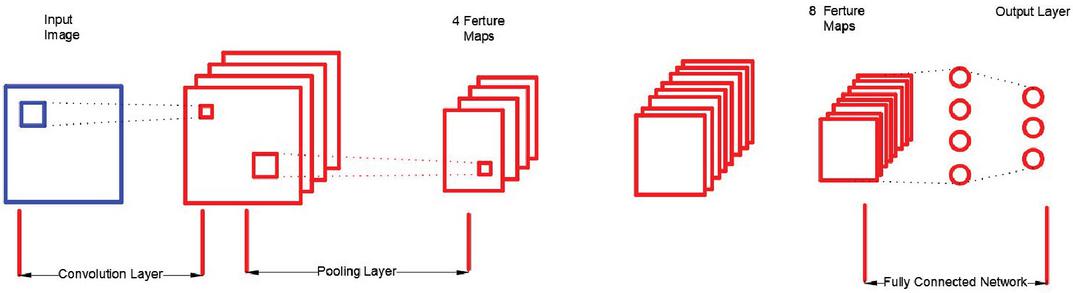
Figure 1 The structure of a CNN.
Figure 1 shows that the CNN generally consists of an input layer, output layers, convolution layers and pooling layers. The neurons in each layer of the network are arranged in three dimensions, and the network also has length, width and height, similar to the cuboid in the geometry. In particular, the neurons of the fully connected layer in the network are arranged in one dimension and are shaped in a straight line [19–22].
The CNN structure shown in Figure 1 has an input layer whose length and width correspond to the width and height of the input image, and its height (also called depth) is 1. The first layer in the convolution layer make convolution for the images in the input network, resulting in several feature maps. Usually, the number of filters in each convolution layer can be set arbitrarily. In other words, the number of filters in the convolution layer is also a parameter. The feature map is actually the image feature obtained by the convolution of the original input image, and the number of filters is equal to the number of feature maps. This makes it possible that several different features can be extracted from the original image.
By assuming an input image size is i*i and then convoluted through a j*j filter, the convoluted feature map is still sized j*j, as shown in Figure 2:
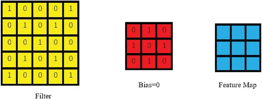
Figure 2 How did convolution work.
The following convolution process was derived by using the following formulas. Because there are many pixels in the image, to simplify the analysis, the pixels of the input image are numbered individually, and the pixel of the image at row and column can be indicated as . Similarly, the weight at row and column in the filter can be denoted as , and the offset term of the filter can be denoted as . Each element of the feature map is numbered, and the element at row and column of the feature map can be represented by . Then, the convolution calculation formula was obtained:
| (1) |
The value of all elements in the feature map can be calculated in turn by Equation (1). In the presented calculation process, the stride was1. The stride can be set to a number greater than 1. For example, when the stride was S, the feature map is calculated as follows:
| (2) | ||
| (3) |
In these two formulas, represents the width of the feature map after convolution; stands for the width of the image before convolution; stands for the width of the filter; represents the number of Zero Padding, which refers to how many laps are needed around the original image; represents the stride; stand for the height of the feature map after convolution; and represents the width of the image before convolution. If the value of the image depth before convolution is , then the depth value of the corresponding filter must also be . By extending Equation (1), a convolution calculation formula with a depth greater than 1 is obtained:
| (4) |
In Equation (4), stands for the depth; F represents the size of the filter (width or height); indicates the weight inline , row , and layer of the filter; indicates the image pixel at the i-th row and the j-th column in the layer . The number of filters at every convolution layer could be greater than 1. For convolution networks with more than one filter, each filter and the original image are convoluted to obtain a feature map [23–25]. The depth (or number) of the Feature Map after convolution is equal to the number of filters in the convolution layer.
3 New Deep-Learning-Network Model
To realize the intelligent recognition of heavy-rail images, a new deep-learning network model with repeated stacking small convolution kernels and a maximum pooling layer was constructed based on the convolution neural network. The model consists of a VGG network and softmax classifier, and its structure is shown in Figure 3.
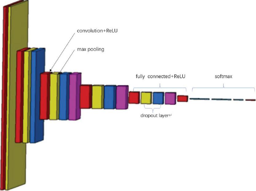
Figure 3 New model of deep-learning network.
The deep-learning network consists of a VGG network composed of five convolution layers and three fully connected layers, all of which are then merged into a new network model with a softmax classifier. VGG net has five convolutions, each of which has two or three convolutions. At the same time, the tail of each segment is connected with a maximum pooling layer to reduce the image size. The number of convolution kernels in each segment is the same, and the later segments have more convolution kernels. The number of convolution kernels in five convolution layers can be expressed as (32,64,12,82,56,512) in vector form. In addition, most of the 3 * 3 convolution kernels in the last three convolutions are the same. These convolution kernels are stacked together in an inverted pyramid shape. In VGG network, multiple 3 3 convolution kernels are used to increase the spatial receptive field and reduce the number of parameters, enhance the ability of non-linear expression, so as to improve the ability of feature learning.
The VGG network uses multiple 3 * 3 convolution kernels to increase the spatial receptive field and reduce the number of parameters and enhance the nonlinear expression capability. Although the parameters of the model are greatly increased compared with the traditional artificial neural network, the number of training iterations of the model is less than the latter. The model itself is highly data-driven, and the structure design of many convolution cores and their alternating connection with the pool layer in the network makes it not strongly dependent on the probability distribution of noise. It is helpful to the anti-noise performance of the network.
The idea of the model for heavy-rail image recognition is that it could extract the heavy-rail image features by the assistance of the VGG network and then use the softmax classifier to quickly classify the extracted features. The classification of heavy-rail images is also a very critical issue, and the accuracy of classification is closely related to the accuracy of the final recognition of image defects.
The image-defect classification is essentially a multi-classification problem, and the expression of the softmax function could be shown as:
| (5) |
is a logarithmic matrix of the probability that a sample belongs to the type defect category; is the probability of the type defect category in the sample image. Then, according to the general linear model, assuming that the model has groups of parameters, then:
| (6) |
is the group parameter in the model, and where represents the sample. For ease of writing, let ; thus, the equation becomes:
| (7) |
Given the sample , the model may have the probability distribution under category :
| (8) |
Equation (8) solves the probability at , where represents probability of corresponding x. In the general linear model of the softmax regression, the objective function is:
| (9) |
The output of the softmax regression objective function is probabilities. After solving this objective function, a classification model can be extracted. The objective function is expressed as follows:
| (10) |
Then, the results above can be used in vector representation, to obtain the following:
| (11) |
Lastly, the final expression of the objective function is
| (12) |
After obtaining the specific expression of the objective function, for training samples, the parameter fitting method can be used to solve the likelihood function.
| (13) |
Then, after is obtained by the gradient descent method, the image defect can be classified using the objective function .
4 Experiment Analysis
To evaluate the recognition ability of the new algorithm to the defect of a heavy-rail image more realistically, the new algorithm described in this work was implemented by using Python 3.7. Normally, there are 16 types of heavy-rail defects that need to be identified in actual production, and the defect list is shown in Table 1.
Table 1 Type of surface defects on heavy-rail
| No. | 1 | 2 | 3 | 4 |
| Scar defects | Scar | Rolling scar | Rolling mark | Meat loss |
| Crack defects | Line pattern | Bottom crack | Crushing | Transverse crack |
| Quenching defects | Folding | Cold injury | Over burning | Correction injury |
| Raised defects | Bulge | Ear | Tumour | Surface inclusion |
Table 1 shows there are many types of heavy-rail surface defects. In the image processing, each defect is cyclically recognized for each picture of the heavy rails. In image processing, every image of the heavy rail is recognized in the cycle, and it is difficult to achieve the ideal result in terms of calculation and time. To address these problems, this work is done by employing the advanced deep-learning-network algorithm to quickly and accurately identify the surface defects of heavy rail.
Before the experiment, the original image [26, 27] was obtained by machine vision. Combined with the surface characteristics of heavy rails and the distribution characteristics of surface defects, the visual system uses colour CCD linear array cameras to collect data on the surface information of heavy rails from various angles. The camera matching method and distribution scheme are shown in Figure 4.
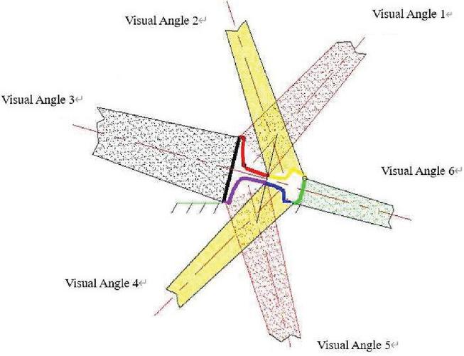
Figure 4 Schematic diagram of camera matching and distribution scheme.
The camera takes pictures of the tread, bottom, upper and lower sides of the heavy rail from six positions. In order to obtain the clear image of the heavy rail surface, it is necessary to filter the light at the entrance of the camera, so as to eliminate the influence of the strong infrared radiation from the center of the hot heavy rail on the information collection of the heavy rail surface. In this paper, the infrared cut-off filter with a cut-off frequency of 800 nm is selected to filter the incident light of the lens. After a period of time, the acquired heavy-rail images were further standardized into 64*64 images for a total of 1200 images, of which 400 were used as learning samples and the rest as test samples. The heavy-rail images exemplified for the experimental sample are shown in Figure 5.
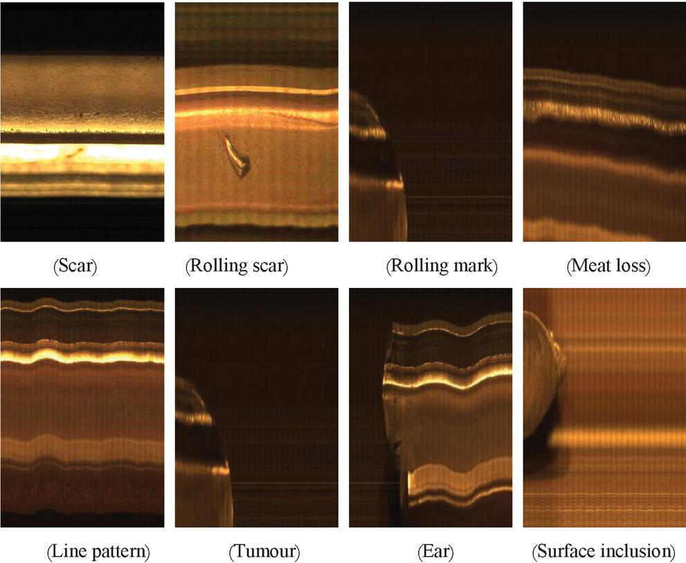
Figure 5
The 400 original images to be learned were inputted into the new deep-learning-network model for training. The network depth was set to 16, and the error rate curve in the training process is shown in Figure 6. After performing the network iteration 35 times, the error recognition rate of training convergence was less than 20%.
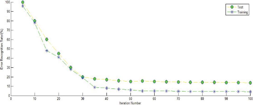
Figure 6 Training process of VGG net.
Then, the remaining samples were identified with a new network model that was trained with an accuracy of more than 95%. In addition, in order to verify the rapidity of the new method. In this paper, Taeguen Algorithm, Yuyongwei, Brachmam and other traditional algorithms are compared and analyzed [28, 29]. The speed of identification of each method is shown in the following Table 2.
Table 2 The recognition speed of each method
| Different | ||||
| Methods | Taeguen Method | Brachmam Method | YuYongWe Method | New Method |
| Time(s) | 32 | 28 | 25 | 12 |
5 Comparative Research
In image processing, the recognition accuracy under noise conditions is an important indicator to measure the superiority of the algorithm. Heavy-rail images are characterized by large grayscale and high-brightness under noise conditions, and they are often required nonlinear processing [30, 31]. In the presence of high noise, even if the signal-to-noise ratio was set too high to make it much larger than the threshold, it was still possible to identify the correct image as a defect feature when using conventional algorithms for image-defect recognition. Processing, in this case, is often referred to as incorrect limit identification (ILI). For example, OPENCV image edge processing and Android digital image processing are both likely to have ILI [32, 33]. In image recognition, the nonlinear pattern recognition method using images such as fractures and cracks may have a large false recognition rate.
To test the performance of the new algorithm in nonlinear image recognition under noise conditions, The comparative study was performed between the new algorithm and the traditional algorithm. Before the comparative analysis, 300 heavy-duty images with noise were selected with the signal-to-noise ratio set to 45 dB and the step size set to 1 to perform ILI. Figure 7 shows the error rate of the new algorithm and the traditional algorithm for heavy-rail image defects under noise conditions.
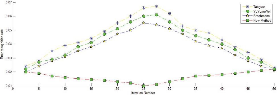
Figure 7 Error rate from various methods under noise conditions.
As shown in Figure 7, the estimation accuracy of the traditional three algorithms under additive noise conditions was very high, and the image-defect-recognition error rate increased with an increased number of iterations. When the step size was set to 1, the TaeGuen algorithm shows the largest error rate of all algorithms under the noise condition. It should be emphasized that, in the above comparative analysis. When the step size is 1 and the signal-to-noise ratio is kept constant, the error probability can be kept stable and declining by adjusting the iteration times. In particular, the error curve first increases to the highest point and then continues to fall and reach a higher level. However, the new method proposed in this paper had almost the same error recognition rate except for a few fluctuations when the number of iterations was in the range [0, 50], and its error rate was the smallest among all the algorithms. When the signal-to-noise ratio was changed to 40 db, in other words, the noise was enhanced, the same number of heavy-rail images was inputted into the network, and the defect recognition error rate was obtained, as shown in Figure 8.
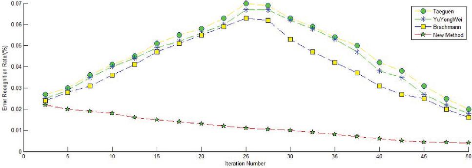
Figure 8 Identification error rate of each method under enhanced noise conditions.
Figure 8 shows that the TaeGuen method presents the largest error rate in all algorithms, and its error rate curve was normally distributed, first high and then low. Surprisingly, Yuyongwei’s algorithm has significantly improved the accuracy of its recognition when the noise was enhanced. The error rate of the new method was always lower than other algorithms in the process of increasing the number of iterations, and when the network iteration for 45 times, its error value did not exceed 5%.
In summary, the simulation results of each algorithm showed that the traditional algorithm had low defect recognition rates under noise conditions. The new method’s false classification rate was the lowest among all algorithms, thus showing its strong anti-ILI performance. In addition,when the noise was larger, the image-defect-recognition rate was still at a higher level for new algorithms, showing its strong nonlinear processing capability. The new algorithm also has other advantages. While the conventional algorithm easily experiences over-fitting because of the noise of the image data, the new method adopts the dropout layer in the middle of the fully connected layer, effectively preventing over-fitting and increasing the robustness of the network.
6 Conclusion
By focusing on the limitations of heavy-rail images, such as noise, over-dark exposure and many types of defects, a new deep-learning-network method featured by a small convolution kernel and maximum pooling layer is proposed based on a convolution neural network. By being simple, fast and practical, the method performs very well in defect recognition for edge-blurred heavy-rail images under noisy conditions, requiring no more iterative calculation. Computer simulation analysis proved the effectiveness of the new algorithm compared with the traditional algorithm for the heavy-rail defect image under noise conditions. In the experimental analysis, the new algorithm can be applied to the correct recognition of heavy-rail defect images and even other fuzzy image defects with noise. Lastly, the paper also discusses the comparison of the error rate between the new algorithm and the traditional algorithm under strong noise conditions. Both the comparative analysis and simulation results show that the new algorithm has a lower recognition error rate when the noise is larger, and it has stronger robustness to ILI. In short, the new algorithm is fully capable of anti-noise and nonlinear performances.
Acknowledgement
This work was supported by the Science Project of Chongqing Municipal Education Commission (Grant no. KJQN201903406) and the Chongqing Research Program of Basic Research and Frontier Technology (Grant no. cstc2018jcyjAX0805).
References
[1] Xie Zhi-jiang, Chen Tao, Chu Hong-yu. The key Technology research of on-line surface inspection for hot heavy rail[J]. Journal of Chongqing University. 2012, 35(3):15–18.
[2] Shi Tian; Kong Jian-yi; Wang Xing-dong. Improved Sobel algorithm for defect detection of rail surfaces with enhanced efficiency and accuracy[J]. Journal Of Central South University, 2016, 23(11):2867–2875.
[3] Ye Suru, Hu Zhimin, Ouyang Qi et al. Research on the Surface Defect Detection System of Heavy Rails Based on Machine Vision [J]. Modern Manufacturing Engineering, 2007, 8:89–90.
[4] E. Sudheer Kumar, C. Shoba Bindu. Two-stage framework for optic disc segmentation and estimation of cup-to-disc ratio using deep learning technique[J]. Journal of Ambient Intelligence and Humanized Computing, 2021, 03:1–7.
[5] Dat Tien Nguyen, Lee, Min Beom, Tuyen Danh Pham. Enhanced Image-Based Endoscopic Pathological Site Classification Using an Ensemble of Deep Learning Models[J]. Sensors, 2020, 20(21):1–16.
[6] Li, Gaoyang, Hong, Yuxiang, Gao, Jiapeng. Welding Seam Trajectory Recognition for Automated Skip Welding Guidance of a Spatially Intermittent Welding Seam Based on Laser Vision Sensor[J]. Sensors, 2020, 20(13):1–6.
[7] Rong, Dian, Wang, Haiyan, Xie, Lijuan. Impurity detection of juglans using deep learning and machine vision[J]. Computers And Electronics In Agriculture, 2020, 178:1–8.
[8] Lu Tao, Wang Jiaming, Li Xiaolin et al. Face Super-resolution Reconstruction Based on Relay Cyclic Residual Network[J]. Journal of Huazhong University of Science and Technology (Natural Science), 2018, 46(12):95–100.
[9] Liu Yongxin, Duan Tiantian. Image Super-resolution Reconstruction Based on Deep Learning [J]. Technology and Innovation, 2018, 23:40–43.
[10] Yu Yongwei, Yin Guofu, Yin Ying et al. A Method for Radiation Image Defect Recognition Based on Deep Learning Network[J]. Chinese Journal of Scientific Instrument, 2014, 35(9):2012–2017.
[11] Chen Tao. Key Technologies for On-line Heavy Rail Detection System for Thermal Surface Defects[D]. Chongqing: Chongqing University, 2011:48–53.
[12] Jin Yuan, Xingxing Hou, Yaoqiang Xiao et al. Multi-criteria active deep learning for image classification[J]. Knowledge-based Systems, 2019, 172:86–94.
[13] Tiago Santos, Stefan Schrunner, Bernhard C. Geiger et al. Feature Extraction From Analog Wafermaps: A Comparison of Classical Image Processing and a Deep Generative Model[J]. IEEE Transactions on Semiconductor Manufacturing, 2019, 32(2):190–198. Zhang, Chuan-Wei, Yang, Meng-Yue, Zeng, Hong-Jun. Pedestrian detection based on improved LeNet-5 convolution neural network[J]. Journal of Algorithms and Computational Technology, 2019, 13:1–9.
[14] Wang, Qibin, Zhao, Bo, Ma, Hongbo. A method for rapidly evaluating reliability and predicting remaining useful life using two-dimensional convolution neural network with signal conversion[J]. Journal of Mechanical Science and Technology, 2019, 33(6):2561–2571.
[15] Madec, Simon, Jin, Xiuliang, Lu, Hao et al. Ear density estimation from high resolution RGB imagery using deep learning technique[J]. Agricultural and Forest Meteorology, 2019, 264:225–234.
[16] Yoshiko Ariji, Motoki Fukuda, Yoshitaka Kise. Contrast-enhanced computed tomography image assessment of cervical lymph node metastasis in patients with oral cancer by using a deep learning system of artificial intelligence[J]. Oral Surgery Oral Medicine Oral Pathology Oral Radiology, 2019, 127(5):458–463.
[17] Mateo Sanguino, Tomas de J., Castilla Webber, Pedro A. Making image and vision effortless: Learning methodology through the quick and easy design of short case studies[J]. Computer Applications in Engineering Education, 2018, 26(6):2102–2115.
[18] Al-Kofahi Yousef, Zaltsman Alla, Graves Robert. A deep learning-based algorithm for 2-D cell segmentation in microscopy images[J]. BMC Bioinformatics, 2018, 19:1–11.
[19] Amato G , Falchi F, Vadicamo L. Visual Recognition of Ancient Inscriptions Using convolution Neural Network and Fisher Vector[J]. ACM Journal on Computing and Cultural Heritage, 2016, 9(4):1–21.
[20] Shibata Naoto, Tanito Masaki, Mitsuhashi Keita. Development of a deep residual learning algorithm to screen for glaucoma from fundus photography[J]. Scientific Reports, 2018, 8:1–9.
[21] Srivastava Arunima, Kulkarni Chaitanya, Huang Kun. Imitating Pathologist Based Assessment With Interpretable and Context Based Neural Network Modeling of Histology Images[J]. Biomedical Informatics Insights, 2018, 10:1–7.
[22] Park Sang Jun, Shin Joo Young, Kim Sangkeun. A Novel Fundus Image Reading Tool for Efficient Generation of a Multi-dimensional Categorical age Database for Machine Learning Algorithm Training[J]. Journal of Korean Medical Science, 2018, 33(43):1–12.
[23] Faust Kevin, Xie Quin, Han Dominick. Visualizing histopathologic deep learning classification and anomaly detection using nonlinear feature space dimensionality reduction[J]. BMC Bioinformatics, 2018, 19:1–15.
[24] Gopalakrishnan Kasthurirangan, Khaitan, Siddhartha K, Choudhary Aloketal. Deep convolution Neural Networks with transfer learning for computer vision-based data-driven pavement distress detection[J]. Construction and Building Materials, 2017, 157:322–330.
[25] Okamura Rintaro, Iwabuchi Hironobu, Schmidt K. Sebastian. Feasibility study of multi-pixel retrieval of optical thickness and droplet effective radius of inhomogeneous clouds using deep learning[J]. Atmospheric Measurement Techniques, 2017, 10(12):4747–4759.
[26] Metcalf SJ (Metcalf, Shari J.), Reilly JM (Reilly, Joseph M.), Kamarainen AM (Kamarainen, Amy M.). Supports for deeper learning of inquiry-based ecosystem science in virtual environments – Comparing virtual and physical concept mapping[J]. Computers in Human Behavior, 2018, 87:459–469.
[27] Yan SY (Yan, Shiyang), Smith JS (Smith, Jeremy S.), Zhang BL (Zhang, Bailing). Action Recognition from Still Images Based on Deep VLAD Spatial Pyramids[J]. Signal Processing-Image Communication, 2017, 54:118–129.
[28] Kim, TaeGuen, Kang, BooJoong, Rho, M (Rho, Mina etal. A Multimodal Deep Learning Method for Android Malware Detection Using Various Features[J]. IEEE Transactions on Information Forensics and Security, 2019, 14(3):773–788.
[29] Brachmann, A , Redies, C. Using convolution Neural Network Filters to Measure Left-Right Mirror Symmetry in Images[J]. Symmetry-Basel, 2016, 8(12):1–10.
[30] Tan Wenxue, Zhao, Chunjiang, Wu, Huarui. Intelligent alerting for fruit-melon lesion image basedonmomentum deep learning[J]. Multimedia Tools and Applications, 2016, 75(24):16741–16761.
[31] Noda, Kuniaki, Arie, Hiroaki), Suga, Yuki. Multimodal integration learning of robot behavior using deep neural networks[J]. Robotics and Autonomous Systems, 2014, 62(6):721–736.
[32] Bansal, Raghav, Raj, Gaurav, Choudhury, Tanupriya. Blur Image Detection using Laplacian Operator and Open-CV[J]. 5th International Conference System Modeling and Advancement in Research Trends (SMART), 2016:63–67.
[33] Farahani, Behzad, V, Barros, Francisco, Sousa, Pedro J. A coupled 3D laser scanning and digital image correlation system for geometry acquisition and deformation monitoring of a railway tunnel[J]. Tunnelling and Underground Space Technology, 2019, 91:1–12.
Biography

Xie Changgui was born in 1984 and obtained Ph.D. in school of mechanical engineering at Chongqing University in December 2012. He is now working as an associate professor in a famous Vocational College in Chongqing. His research area is about equipment diagnosis and signal processing, artificial intelligence etc. He has presided over many national and provincial projects.
Journal of Web Engineering, Vol. 20_5, 1623–1640.
doi: 10.13052/jwe1540-9589.20513
© 2021 River Publishers