Mining Simple Path Traversal Patterns in Knowledge Graph

Feng Xiong and Hongzhi Wang^*

Department of Computer Science, Harbin Institute of Technology, China

E-mail: fxiong@hit.edu.cn; wangzh@hit.edu.cn

$^{*}$ Corresponding Author

Received 19 July 2021; Accepted 16 August 2021; Publication 03 January 2022

Abstract

The data mining has remained a subject of unfailing charm for research. The knowledge graph is rising and showing infinite life force and strong developing potential in recent years, where it is observed that acyclic knowledge graph has capacity for enhancing usability. Though the development of knowledge graphs has provided an ample scope for appearing the abilities of data mining, related researches are still insufficient. In this paper, we introduce path traversal patterns mining to knowledge graph. We design a novel simple path traversal pattern mining framework for improving the representativeness of result. A divide-and-conquer approach of combining each path is proposed to discover the most frequent traversal patterns in knowledge graph. To support the algorithm, we design a linked list structure indexed by the length of sequences with handy operations. The correctness of algorithm is proven. Experiments show that our algorithm reaches a high coverage with low output amounts compared to existing frequent sequence mining algorithms.

Keywords: Knowledge graph, path traversal, data mining.

1 Introduction

The advancement of the Mobile Internet increases the likelihood of completely realizing the Internet of Everything. The amount of data created as a result of such interconnectivity has skyrocketed, and it might be used as useful raw materials for relation analysis. Aside from the prior emphasis on each individual in terms of intellectual analysis, the relations between each will definitely become significant as a result of the Mobile Internet age. Fortunately, Knowledge Graph might be useful as long as there is a need for relation analysis.

Knowledge graph is a repository that is constructed by semantic networks in essence, and it could be seen as a multi-relation graph. Introducing path traversal patterns mining algorithms to knowledge graph promotes efficiency. For instance, in a knowledge graph of investor relations researchers use frequent supply chain partners to analyze the cause of relationship-specific asset [19]. Path traversal patterns mining algorithms could help obtain possible passes from data compression graph [23]. The intention to identify suitable documents by extracting a knowledge graph of relations from a large scientific dataset requires frequent path traversal patterns relations [1].

Additionally, loops are always not welcomed in such graph. According to the survey, it is commonly observed that the 96% of loops in Probase [36] have wrong isA relations [18]. Removing loops from the Wikipedia graph when constructing a primary taxonomic tree is imperative [9]. A loopless knowledge graph that is told facts about what is true in the world is often a sign of a bug [26]. Therefore, developing the research of simple path (path without loops) [12, 13, 40] traversal patterns mining in knowledge graph is imperative.

However, the appropriative research of simple path traversal patterns on knowledge graph is absent. Even though we may utilize several classic algorithms to handle this issue, such as GSP [32], Spade [41], PrefixSpan [24], Spam [2], they could not satisfy well. The vulnerability of such algorithms is that they could produce frequent subsequences from a graph which is constructed by a training set, but they could not produce frequent simple path traversal patterns from it. Furthermore, we could modify path traversal patterns mining algorithms [5, 21] for mining path traversal patterns from knowledge graph, the additional cost for loop computation could decrease the efficiency.

To determine the frequency of simple path, We introduce an evaluation parameters Coverage. Coverage is accumulated by each sequence of traversal data, which is a subsequence of other sequences. The sufficiency of a set of frequent sequences could be determined by its Coverage because one covers and represents most sequences in the training set. We consider Coverage as a critical parameter to measure the effectiveness of an algorithm for producing frequent sequences on knowledge base. To illustrate the point, we give a naive example.

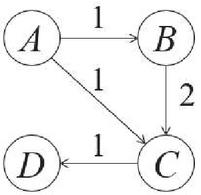
Figure 1 An example of a naive knowledge graph.

We have four entities $A, B, C, D$ in an knowledge graph $G$ . There are three sequences in the training set, in which one sequence $< A, B, C >$ is used to build relations between $A, B, C$ , where $A$ is directly related to $B$ , $B$ is directly related to $C$ . We also have such two sequences $< B, C, D >$ and $< A, C >$ in the training set. Together, a naive knowledge graph $G$ is build by the training set as shown in Figure 1 where the number on each edge tells the total frequency of relations between each pair of entities. We want to discover frequent sequences in $G$ . Classic frequent sequential patterns mining algorithms would give the result that there are two sequences, $< B, C >$ and $< A, C >$ , who have a support of 2 sequences. However, there is a longer sequence $< A, B, C, D >$ which is a substructure of $G$ despite it has a support of only 1 sequence. This sequence represents all of three sequences $< A, B, C >$ , $< B, C, D >$ and $< A, C >$ , namely it has a Coverage of 3 sequences. Hence one can see that Coverage is significative and valuable to determine if a sequence of traversal data in knowledge graph is frequent enough.

In this paper, we study simple path traversal mining problem on acyclic knowledge base. With the intention of gaining high Coverage, we develop a novel framework containing both data structure and algorithm, which is different from all classic sequential pattern mining algorithms. The structure indexing the length of each sequence to support the algorithm is concise and easy to operate. The algorithm aims to produce a set of frequent sequences of traversal data with high Coverage through combining each sequence of different length, which is efficient and effective. To ensure the efficiency, we design the combining process in a divide-and-conquer manner and the pruning strategy to accelerate it. To ensure the effectiveness, we combine sequences in the priority of sequence length and support resulting in a small set of generated simple path traversal patterns with high Coverage.

The contributions of this paper are summarized as follows.

• We study the simple path traversal patterns mining problem on knowledge base with Coverage as the optimization goal. As we know, this is the first paper that studies this problem.

• To discover high-coverage paths, we design a novel algorithm that considers both the length and frequency of the discovered results. For the consideration of efficiency, we combine sequences of traversal data in a divide-and-conquer approach. We prove that our algorithm achieves the goal of problem by reasoning.

• In this algorithm, we add pruning strategy facing to not only the frequency but also the Coverage. We also design a linked list for the sequences indexed by their lengths to support the algorithm efficiently.

• Extensive experimental results on real data sets show that the proposed approach could discover simple path traversal patterns on knowledge graph with high coverage efficiently.

The rest of the paper is organized as follows. Section 2 introduces the preliminaries, problem definition, and the outline of algorithm. Section 3 illustrates the data structure with its maintenance operations. Section 4 introduces algorithms of sequences combination. In Section 5, we design the algorithm, and its pruning strategies. We prove the correctness of algorithm by reasoning. Section 6 shows the result of our experiments. Section 7 discusses the related work of the problem. Section 8 draws the conclusions and presents an expectation of our work.

2 Overview of Algorithm

In this section, we introduce the basic definitions related to the problem. After that we determine the definition and optimization goals of our problem. Finally, the outline of our algorithm is given to make our work easier to understand.

2.1 Basic Definitions

A simple path traversal patterns is modeled as a sequence, which is an ordered list of elements denoted by $s = < e_{1}, \dots, e_{n} >$ , where $e_{1} \neq e_{n}$ because the path should be simple. The length of a sequence $s$ is the number of elements in $s$ , denoted by $| s |$ . A sequence $s_{j}$ is a subsequence of another sequence $s_{i}$ iff the set of ordered element in $s_{j}$ is a subset of that in $s_{i}$ , denoted by $s_{j} ⊏ s_{i}$ . Also, $s_{j}$ is a subsequence of $s_{i}$ . Given two sequences $s_{i} = < a_{1}, \dots, a_{n} >$ and $s_{j} = < b_{1}, \dots, b_{m} >$ , formally we have the following definitions.

Definition 1. $s_{j} ⊑ s_{i}$ iff there exists integers $1 \leq x_{1} < \dots < x_{m} \leq n$ such that $b_{1} = a_{x_{1}}, \dots, b_{m} = a_{x_{m}}$ .

Definition 2. $s_{j} ⊏ s_{i}$ iff $s_{j} ⊑ s_{i}$ and $s_{j} \neq s_{i}$ .

For example, we describe the sequences of marital status as follows.

Example 1. Consider five elements $e_{1}, e_{2}, e_{3}, e_{4}, e_{5}$ , and three sequences $s_{1} = < e_{1}, e_{2}, e_{3} >$ , $s_{2} = < e_{1}, e_{2}, e_{4} >$ , $s_{3} = < e_{1}, e_{2}, e_{4}, e_{5} >$ , we notice that $s_{2} ⊏ s_{3}$ .

We denote $D$ as a training set containing a set of sequences such that $D = {s_{1}, \dots, s_{n}}$ . The acyclic knowledge base is a directed acyclic graph $G = (V, E)$ constructed by $D$ , where $V$ is a set of vertices that $\forall v^{'} \in V$ , $v^{'} \in s_{i}$ and $E$ is a set of edges that $\forall e^{'} = < v^{'}, v^{''} > \in E$ , $< v^{'}, v^{''} >$ is an adjacent pair in $s_{i}$ .

2.2 Problem Definition

In this paper, we focus on simple path traversal patterns mining problem. In order to achieve an unsupervised process effectively and efficiently, we have three demands of the problem as follows. Note that these requirements are not incompatible and we prove that our approaches achieve these demands later.

Maximize coverage. Coverage is accumulated by each sequence of traversal data, which is a subsequence of one of resulted sequences in the knowledge graph. The resulted set of frequent sequences covering and representing most sequences in the training set always has high Coverage. Thus, the sufficiency of the resulted set of frequent sequences could be determined by its Coverage. This is the main optimization goal of the problem.

Maximize length of rules. Because a longer sequence could cover more paths in the knowledge base and our algorithm is on the basis of combining, it is necessary to reduce the size of set of sequences for efficiency and effectiveness. Besides, retrench the size of the set of frequent sequences could make one more representative and help save both of internal and external storage space.

Ensure rules are frequent. We should ensure the support of all sequences are over a predefined threshold. This will make the generated sequences frequent enough. Then, our result could benefit from it and obtain frequent sequences from the knowledge base. This improves the usability of the resulted set of frequent sequences.

Based on these requirements, we give a formal definition of our problem. We denote $D$ as the input and $T$ the result. $D$ is a set containing a number of sequences such that $D = {s_{1}, \dots, s_{n}}$ . Then, we denote one resulted sequence by a pattern $t_{i}$ . For each pattern $t_{i}$ , its compatible set in $D$ is denoted by $S_{t_{i}}^{D}$ such that $S_{t_{i}}^{D} = {s_{i} | s_{i} ⊏ t_{i}, s_{i} \in D}$ . $T$ is a set of such patterns that $T = {t_{1}, \dots, t_{i}, \dots, t_{m}}$ . Finally, the coverage of $T$ is $| ⋃_{t_{i} \in T} S_{t_{i}}^{D} |$ . To compare the Coverage among different results without loss of generality, we define the rate of Coverage of $T$ as

c o v = \frac{| ⋃_{t_{i} \in T} S_{t_{i}}^{D} |}{| D |}

Problem. For the input $D$ , the goal of the problem is to obtain a proper pattern set $T$ from $D$ , that satisfies the following three conditions.

• Maximize $c o v (T)$ , and

• Maximize $\frac{Σ | t_{i} |}{| T |}$ , the average length of sequences in $T$ , and

• For each $t_{i} \in T$ , $| S_{t_{i}}^{D} | \geq ϵ_{f}$ , where $ϵ_{f}$ is the threshold of the pattern frequency.

As above, three conditions meet the demands of the problem. In this paper, we design the data structure and algorithms around this problem. And we prove how our algorithms meet these three conditions in Section 5.2.

3 Data Structure

To support effective and efficient currency rule discovery, we develop a specific data structure of the sequence set $D$ . Based on above discussions, the basic elements in our data structure named FSGroup are sequences with their support. FSGroup has two basic operations as follows.

• (Insert.) Inserting a sequence into the structure with its support.

• (Delete.) Deleting a sequence and remove its entry from the structure.

Additionally, the data structure should support the sequential access of sequences with the same length one by one. Note that the combination of two sequences, which is an important operation in the algorithm, is implemented with these operations, and will be discussed in Section 4. In this section, we focus on the structure (in Section 3.1) and the implementation algorithms of these basic operations (in Section 3.2).

3.1 Storage Structures

Since a longer sequence contains more elements than the shorter, the coverage of the former is higher than the latter. Thus, the combine operation on $D$ is on the longest and second longest sequence. To support these operations, the sequences are grouped by their lengths. We use a linked list to store the sequences with the same length for the efficiency of insert and delete operation. To access the sequences with the specific length, we group the heads of all linked lists as an array and index the heads with the lengths of sequences in the linked lists. Formally, the structure is defined as follows.

Definition 3. A FSGroup contains following three components.

• Groups of linked lists, denoted by $B$ . Each linked list represents the set of sequences with the same length. Each entry in a linked list is a triad $(s e q, c o u n t, n e x t)$ where $s e q$ is a sequence, $c o u n t$ the support of $s e q$ , and $n e x t$ the pointer to the next entry.

• A pair of length information $P = (p l e n, m l e n)$ , where $p l e n$ predefines the maximum length of the combined sequences, and $m l e n$ is the maximum length of all sequences.

• An array for head nodes of all linked lists, denoted by $H$ . Head node $h_{i}$ , $i = [2 \dots P . p l e n]$ indicates the head of the linked list of all sequences with length $i$ .

In summary, we describe the data structure as a triad.

L = (B, P, H)

where $L$ is the structure of $D$ , $B$ its set of sequence entries, $P$ its additional properties, $H$ its index table of linked lists. The additional space consumption is the index table, of which the length is considered to be the maximum length of combined sequences. Moreover, It is convenient for using this structure because sequences with high supports are also longer than others. Therefore, we could only visit the big end of the index table $H$ when we retrieve the final result of all combinations. The structure is demonstrated in Figure 2.

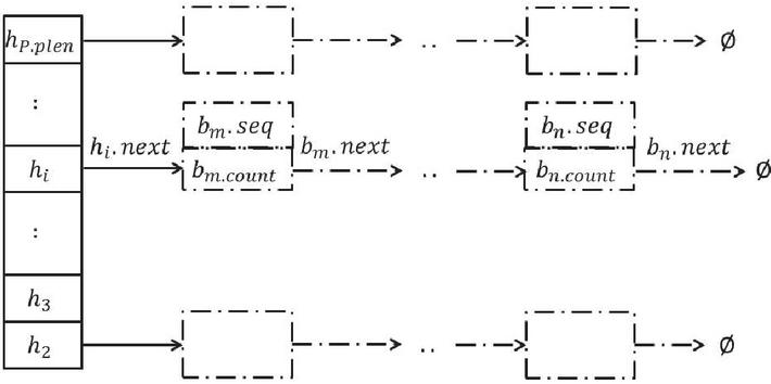
Figure 2 Illustrative diagram of $L$ .

3.2 Operations

In this section we introduce basic operations in $L$ to support our algorithms. Since we can search a sequence directly by its length, we only need two operations including insert and delete. The time complexity of insert operation is $O (n)$ and delete $O (1)$ , such that it is easy to use the data structure we devise.

Insert. The insert operation is accomplished by function FSGInsert $(L, b_{m})$ , which inserts an entry $b_{m}$ into $L$ in accordance with its length. We insert $b_{m}$ into the proper position to ensure that the support of nodes in the linked listed pointed by $h_{| b_{m . s e q} |}$ are in a monotone decreasing single linked list.

Algorithm 1 FSGInsert algorithm

1: function FSGInsert $(L, b_{m})$

2: $p \leftarrow L . h_{| b_{m . s e q} |}$

3: while $p . n e x t . c o u n t > b_{m} . c o u n t$ do

4: $p \leftarrow p . n e x t$

5: $b_{m} . n e x t \leftarrow p . n e x t$

6: $p . n e x t \leftarrow b_{m}$

7: end while

8: end function

The pseudocode of this algorithm is shown in Algorithm 1. Line 2 obtains the head node of the linked list indexed by the length of input sequence. Lines 3–4 find the proper position where we insert the entry to keep monotone decreasing. Lines 5–6 insert $b_{m}$ into the linked list $L$ .

Delete. We delete the a sequence by using the basic delete operation of linked list structure. We invoke function FSGDelete $(L, b_{m})$ to delete an entry $b_{m}$ in $L$ to avoid repeated computation after $b_{m}$ has been indicated as used during a merge or combine operation. This operation could save the storage space.

4 Combination of Sequences

In this section, we propose methods to combine sequences effectively and efficiently. It is crucial for the combine operation because it generates a long sequence of two sequences that meets the requirements. We implement this in a divide-and-conquer approach. For this task, we define two operations, merge and combine. The former fuses a sequence into its supersequence. The latter generates the supersequence of two sequences which overlap but do not contain each other. We will discuss these two operations in Sections 4 and 4.2, respectively.

4.1 Merge Operation

With regard to $b_{m}$ and $b_{n}$ , two entries in $L$ with $b_{m} . s e q ⊏ b_{n} . s e q$ , the merge operation merges $b_{m}$ into $b_{n}$ . Concretely, this operation delete $b_{m}$ and add the support of $b_{m}$ to $b_{n}$ . Since $b_{m} . s e q ⊏ b_{n} . s e q$ , $b_{n} . s e q$ , does not change in this operation.

Algorithm 2 FSMerge algorithm

1: function FSMerge $(L, b_{n}, b_{m})$

2: $b_{n} . c o u n t \leftarrow b_{n} . c o u n t + b_{m} . c o u n t$

3: FSGDelete $(L, b_{m})$

4: return $b_{n}$

5: end function

The pseudocode of merge operation is shown in Algorithm 2. Line 2 accumulates the support of $b_{m}$ to $b_{n}$ . Then in Line 3, we delete $b_{m}$ . The time complexity of this operation is $O (1)$ .

4.2 Combine Operation

Given $b_{m}$ and $b_{n}$ , two entries in $L$ , the combine operation combines them into one new entry $b_{f}$ , where $b_{f} . s e q$ contains all elements in both $b_{m} . s e q$ and $b_{n} . s e q$ , and satisfies $b_{m} . s e q ⊏ b_{f} . s e q$ and $b_{n} . s e q ⊏ b_{f} . s e q$ . We will discuss the implementation algorithm for this operation in this section. At first, we overview the implementation in Section 4.2.1 and then we describe the steps in detail in Sections 4.2.2, 4.2.3, and 4.2.4, respectively.

4.2.1 Algorithm overview

Combine operation attempts to get the “union” of $b_{m} . s e q$ and $b_{n} . s e q$ . However, the union of two sequences is different to that of sets due to the order of elements in the sequence. Consider a brief example. $s_{1} = < h, A, t >$ , and $s_{2} = < h, B, t >$ . The longest common sequence (LCS for short) of $s_{1}$ and $s_{2}$ is $< h, t >$ . Between $h$ and $t$ , $s_{1}$ contains the subsequence $< A >$ while $s_{2}$ contains the subsequence $< B >$ . The results of the combination should be a sequence. It is a problem how to combine such different subsequences between common sequences.

As simple path traversal patterns mining requires frequent sequences, the combination of two different subsequences should maximize the frequency of the result. Thus, we attempt to choose the order of the elements in different sequences with the highest frequency among all possible combinations. In the example above, if the frequency of subsequence $< A, B >$ is larger than that of $< B, A >$ in the whole sequence set $D$ , we should choose $< A, B >$ in the combination result. As a result, the combination of $s_{1}$ and $s_{2}$ is $< h, A, B, t >$ .

To state our approach formally, we first introduce some concepts. We split two sequences $s_{1}$ and $s_{2}$ into two kinds of parts, common parts and alien parts, as introduced in Definition 4.

Definition 4. For two sequences $s_{1}, s_{2}$ , if there exists a continues sequence $t$ , $t ⊑ s_{1}, t ⊑ s_{2}$ and does not exists any subsequence $t *, t ⊏ t^{*}, t^{*} ⊑ s_{1}, t^{*} ⊑ s_{2}$ , we call $t$ a common part. In $s_{1}$ or $s_{2}$ , if there exists a sequence $t^{'}$ between two common parts, then $t^{'}$ is called an alien part.

We use an example to illustrate this concept.

Example 2. For two sequences $s_{1}$ and $s_{2}$ that $s_{1} = < h, A, B, F, G, K, I, t >, s_{2} = < h, C, D, E, F, G, I, J, t >$ , their common and alien parts are shown in Figure 3.

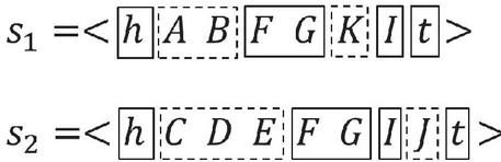
Figure 3 Common and alien parts in $s_{1}$ and $s_{2}$ .

Intuitively, $s_{1}$ and $s_{2}$ share same common parts and their common parts form their largest common sequence. Thus, common parts of two sequences could be generated by the largest common sequence generation algorithm [6]. Then, two sequences are split into several parts according to the common parts. Between two consecutive common parts, each continuous part is an alien part. After this step, each sequence is split into a series of common parts and alien parts and could be represented as the form $< h, t_{1}, \dots, t_{i}, \dots, t_{n}, t >$ , $t_{i} ⊏ s$ , $i \in [1 \dots n]$ , where $t_{i}$ is either a common part or an alien part. $h$ and $t$ identify the head and tail of sequence, respectively.

With this definition, we may discuss the specifics of the combine operation’s implementation methods. This method integrates related common and alien components into a single algorithm. Since the more complex step is the combination of alien parts, we discuss AlienCombine algorithm in Section 4.2.2 at first. Then based on the AlienCombine algorithm, we propose PartCombine algorithm in Section 4.2.3. PartCombine algorithm combines both common parts and alien parts. In order words, it includes three conditions, one of which is processed by AlienCombine algorithm. At last, with PartCombine algorithm as the core step, the whole algorithm, FSCombine algorithm is introduced in Section 4.2.4. The relationship of these algorithms is shown in Figure 4.

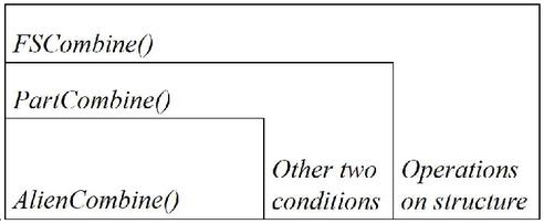
Figure 4 Skeleton of combine operation.

4.2.2 AlienCombine algorithm

In this section, we discuss the implementation of AlienCombine step. As discussed above, the combination of two alien parts selects their element order with frequency.

To make the selection, we attempt to combine the elements in two alien parts in sort-merge style. That is, we use two cursors, $c_{1}$ and $c_{2}$ , pointing to the processing elements in two alien parts $t_{1}$ and $t_{2}$ . If the frequency of $< c_{1}, c_{2} >$ is larger than that of $< c_{2}, c_{1} >$ , $c_{1}$ is selected as an element of the combined sequence and the cursor in $t_{1}$ moves to the next. The process continues until the cursor points to the tail of one sequence and the remaining elements of the other are concatenated to the tail of the generating sequence.

To compare the elements according to the sequence frequency, we define the weight of element pair in Definition 5 and give a brief example in Example 3.

Definition 5. Let $Γ (e_{i}, e_{j})$ denote the total support of the subsequence $s_{s u b} = < e_{i}, e_{j} >$ That is, $Γ (e_{i}, e_{j}) = | {s | s \in D \land s_{s u b} ⊑ s \land e_{i}, e_{j}$ are adjacent in $s} |$ .

Example 3. Let $D = {s_{1}, s_{2}, s_{3}}$ , where $s_{1} = < A, B >$ , $s_{2} = < A, B, C >$ , $s_{3} = < A, B, C, D >$ . Thus, $Γ (A, B) = 3$ , $Γ (B, C) = 2$ , $Γ (C, D) = 1)$ , $Γ (A, C) = 0$ and $Γ (B, A) = 0$ .

Algorithm 3 AlienCombine algorithm

1: function AlienCombine $(t_{1}, t_{2})$

2: $O u t \leftarrow \emptyset$

3: $c_{1} \leftarrow t_{1} [0], c_{2} \leftarrow t_{2} [0]$

4: while $c_{1} \neq \emptyset$ or $c_{2} \neq \emptyset$ do

5: if $Γ (c_{1}, c_{2}) > Γ (c_{2}, c_{1})$ then

6: $O u t \leftarrow O u t + c_{1}$

7: $c_{1} \leftarrow c_{1} . n e x t$

8: else

9: $O u t \leftarrow O u t + c_{2}$

10: $c_{2} \leftarrow c_{2} . n e x t$

11: end if

12: end while

13: while $c_{i} \neq \emptyset, i = 1, 2$ do

14: $O u t \leftarrow O u t + c_{i}$

15: $c_{i} \leftarrow c_{i} . n e x t$

16: return $O u t$

17: end while

18: end function

Based on the weight function, the pseudocode of this algorithm is shown in Algorithm 3, where we use $+$ to represent the concatenation of sequences. For instance, if $s = < a, b >$ and $t = < c, d, e >$ , $s + t = < a, b, c, d, e >$ . Line 2 initiates the output. Line 3 points the cursors to the head elements of two sequences, respectively. Lines 4–10 judge which cursor should be concatenated to the result $O u t$ , then move the cursor to the next, until one is pointed to $\emptyset$ , the tail. Lines 11–13 output rest of elements to $O u t$ orderly. As a result, Line 14 returns the combination of two alien parts.

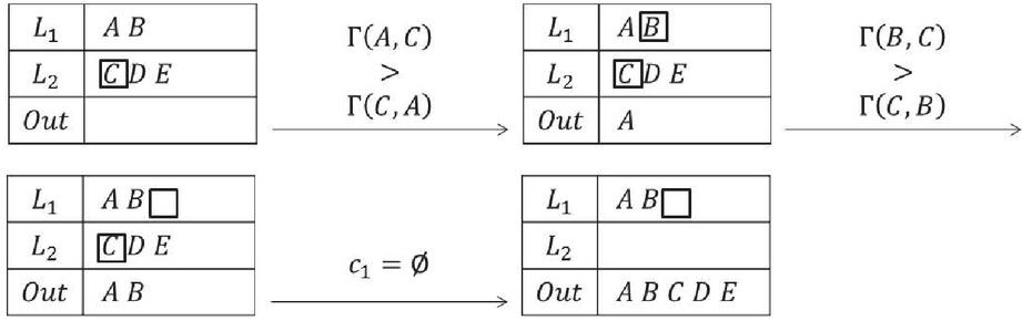
Figure 5 An example of combining two alien parts.

Example 4. We use the example shown in Figure 5 to demonstrate the proposed algorithm. Firstly, the cursor $c_{1}$ and $c_{2}$ are pointed to head of $t_{1} = < A, B >$ and $t_{2} = < C, D, E >$ , respectively. We suppose $Γ (A, C) > Γ (C, A)$ , so we choose the element $A$ and move $c_{1}$ to the next. Then we suppose $Γ (B, C) > Γ (C, B)$ , so we select $B$ and move $c_{1}$ to the next. Noticing that $c_{1}$ points to the tail of $t_{1}$ , we orderly output rest of elements in $t_{2}$ . Finally, we get the result in $O u t$ as shown.

Since this operation is implemented in a divide-and-conquer approach, the time complexity is reduced from $O (m n)$ to $O (m + n)$ where $m$ and $n$ denote the length of input sequences, respectively. To simplify representation of time complexity, we let $m$ denote the max length of two sequences. The time complexity is $O (m)$ . Property 1 demonstrates the correctness of this strategy. $A \to B$ means $A$ and $B$ are adjacent in the sequence combined.

Property 1. For two alien parts $s = < e_{1}, \dots, e_{i}, \dots, e_{n} >$ , $t = < f_{1}, \dots, f_{j}, \dots f_{m} >$ , $\forall e_{i} \in s$ , if $\exists f_{j} \in t$ , $e_{i} \to f_{j}$ , we have $e_{i} \to f_{j^{'}}$ , $j^{'} \in [(j + 1) \dots m]$ , vice versa.

Proof. We use contradiction. Suppose $f_{j + 1} \to e_{i}$ . Because of $f_{j} \to f_{j + 1}$ and $e_{i} \to f_{j}$ , these three paths form a cycle, which is contradict to our statement of breaking the cycle in Section 2.1. Hence we have $e_{i} \to f_{j} \Rightarrow e_{i} \to f_{j + 1} \Rightarrow \dots \Rightarrow e_{i} \to f_{m}$ .

4.2.3 PartCombine algorithm

In this section, we propose the algorithm to combine both common parts and alien parts. Generally, the combination of two sequences $s_{1}$ and $s_{2}$ may involve following three conditions.

• A common part $s^{'}$ of $s_{1}$ and $s_{2}$ . $s^{'}$ is included in the result of combination, and

• An alien part $s_{i}$ in one sequence without a corresponding alien part in the other sequence. That is, for two common parts $s_{i - 1}$ and $s_{i + 1}$ , $s_{1} = < h, \dots, s_{i - 1}, s_{i}, s_{i + 1}, \dots, t >$ and $s_{2} = < h, \dots, s_{i - 1}, s_{i + 1}, \dots, t >$ . In this case, the combination result is $< h, \dots, s_{i - 1}, s_{i}, s_{i + 1}, \dots, t >$ , and

• Two alien parts $s_{i}$ and $s_{j}$ share the same adjacent common parts. That is, for two common parts $s_{i - 1}$ and $s_{i + 1}$ , $s_{1} = < h, \dots$ , $s_{i - 1}$ , $s_{i}, s_{i + 1}, \dots, t >$ and $s_{2} = < h, \dots, s_{i - 1}, s_{j}, s_{i + 1}, \dots, t >$ For this case, we invoke Algorithm 3 to combine $s_{i}$ and $s_{j}$ .

Example 5. We use an example to demonstrate these three conditions in Figure 6, where the number below each block shows the case of the part.

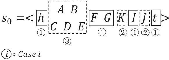
Figure 6 Three conditions in $s_{0}$ .

Considering all these three cases, we design PartCombine algorithm as depicted in Algorithm 4. In this algorithm, we also use $+$ to represent the concatenation of sequences as in Algorithm 3.

Algorithm 4 PartCombine algorithm

1: function PartCombine $(s_{1}, s_{2})$

2: $L C S (s_{1}, s_{2})$

3: $c_{1} \leftarrow s_{1} . h, c_{2} \leftarrow s_{2} . h, O u t \leftarrow \emptyset$

4: while $c_{1} \neq t$ and $c_{2} \neq t$ do

5: if $c_{1}$ is common then

6: $O u t \leftarrow O u t + c_{2}$

7: $c_{2} \leftarrow c_{2} . n e x t$

8: if $c_{2}$ is common then

9: $c_{1} \leftarrow c_{1} . n e x t$

10: else

11: $c_{1} \leftarrow c_{1} . n e x t$

12: if $c_{2}$ is common then

13: $O u t \leftarrow O u t + c_{1}$

14: else

15: $O u t \leftarrow O u t + A l i e n C o m b i n e (c_{1}, c_{2})$

16: $c_{2} \leftarrow c_{2} . n e x t$

17: end if

18: end if

19: end if

20: end while

21: return $O u t$

22: end function

Initially, these two sequences are partitioned into common parts and alien parts with the longest common sequence algorithm (in Line 2). Then the parts are combined in a merge style. We use two cursors, $c_{1}$ and $c_{2}$ , pointing to the processing parts of $s_{1}$ and $s_{2}$ , respectively. Line 3 initiates the two cursors and the output. Lines 4–16 iteratively process parts pointed by cursors until one of which points to the tail of $s_{1}$ or $s_{2}$ . We obtain the output of this function, namely, the result of combining two sequences in Line 18. In detail,

• When the part in $c_{1}$ is a common part but that in $c_{2}$ is an alien one (Line 5), we concatenate the part pointed by cursor $c_{2}$ , then move it to the next (Lines 6, 7).

• When the both of parts in $c_{1}$ and $c_{2}$ are common parts (Lines 5, 8), we concatenate the any part (because they are the same as stated to the result, then move both cursors $c_{1}$ and $c_{2}$ to the next (Lines 6, 7, 9).

• When the both of parts in $c_{1}$ and $c_{2}$ are alien parts (Lines 10, 14), we invoke AlienCombine Algorithm to combine two alien parts, the output of which is concatenated to the result. Then we move both cursors $c_{1}$ and $c_{2}$ to the next (Lines 11, 15, 16).

The time complexity of this operation is still $O (m)$ because the time complexity of all three conditions are $O (m)$ .

4.2.4 FSCombine algorithm

To combine two entries $b_{m}$ and $b_{n}$ in $L$ , besides the combination of sequences $b_{m} . s e q$ and $b_{n} . s e q$ with PartCombine Algorithm discussed in Section 4.2.3, we also need to delete entries $b_{m}$ and $b_{n}$ , add theirs supports to the combined entry $b_{f}$ , and insert $b_{f}$ to corresponding list.

Algorithm 5 FSCombine algorithm

1: function FSMerge $(L, b_{n}, b_{m})$

2: $b_{f} . s e q \leftarrow PartCombine (b_{n} . s e q, b_{m} . s e q)$

3: $b_{f} . count \leftarrow b_{n} . count + b_{m} . count$

4: FSGInsert $(L, b_{f})$

5: FSGDelete $(L, b_{m})$

6: FSGDelete $(L, b_{n})$

7: return $b_{f}$

8: end function

The pseudocode is shown in Algorithm 5. Line 2 gets the result of combination from function PartCombine as mentioned before. Line 3 accumulates the support from two subsequences to the new entry. Line 4 inserts the new entry $b_{f}$ to $L$ . Lines 5–6 delete two old entries $b_{m}$ and $b_{n}$ , respectively. Line 7 returns $b_{f}$ .

The upper bond of time complexity of this algorithm is $\max {O (m), O (l)}$ , where the time complexity of PartCombine is $O (m)$ , with the maximum length of input sequences denoted by $m$ , and that of FSGInsert is $O (l)$ with the maximum length of sequence blocks in linked lists of $L$ denoted by $l$ .

5 The CFSM-AKB Algorithm

In this section, we propose the CFSM-AKB (Coverable Frequent Sequence Mining on Acyclic Knowledge Base), with the data structure and algorithms introduced above (in Section 5.1). Then we demonstrate the correctness of CFSM-AKB (in Section 5.2).

5.1 CFSM-AKB Algorithm

To achieve the goal of problem, in this section, we propose the CFSM-AKB algorithm. In this algorithm, all sequences are stored in a FSGroup $L$ introduced in Section 3.1. The algorithm iteratively combines long sequences by invoking the FSCombine algorithm introduced in Section 4.2.4.

Initially, all input sequences with same length are grouped respectively. Then $L$ is constructed according to these groups by invoking FSGInsert. In the algorithm, groups in $L$ are identified as $g_{1}, \dots, g_{l}$ , $g_{i}$ is the linked list for the sequences with the $i$ th shortest lengths. Since the longer sequences may be generated and some groups may be withdrawn, $l$ and the subscript of some groups will change accordingly during the algorithm.

During the algorithm, we use a cursor $c$ to point to the processing entry. In the beginning, $c$ pointing to the head of the active group with the second longest length $g_{l - 1}$ .

In each round, the precondition is that the entry $b_{i}$ pointed by $c$ is in the group $g_{j}$ . It is decided whether $b_{i}$ should be merged (but not combined) into entries in $g_{j + 1}, \dots, g_{l}$ . After $b_{i}$ is processed, the increasing of the length of the longest sequence means that the current group with the second longest length is not $g_{l - 1}$ , and we denote current one by $g_{t}$ . Then $c$ moves to the head of $g_{t}$ . Otherwise, $c$ moves to the next entry in $g_{j}$ . If all entries in $g_{j}$ are processed, $c$ moves to the head of $g_{j - 1}$ . The algorithm halts when the longest length of sequences does not change and the tail of $g_{1}$ has been processed.

The merge or combination operation is applied on the entries according to the relationship of their sequences. For an example, for $b_{i}$ pointed by $c$ , if $\exists b_{k}$ , $b_{i} . s e q$ is a subsequence of $b_{k} . s e q$ , then $b_{i}$ is merged into $b_{k}$ . Let $g_{j +}$ denote the set of all the entries in groups $g_{j + 1}, \dots, g_{l}$ such that $g_{j +} = {b | b \in g_{i}, i \in [(j + 1) \dots l]}$ . If one entry $b_{i}$ in $g_{j}$ could be merged with multiple entries $b_{k_{1}}, \dots, b_{k_{u}}$ in $g_{j +}$ , we first merge $b_{i}$ into any entry $b_{k_{i}}$ , then combine these multiple entries two by two. In other words, FSCombine $(b_{k_{i}}, b_{k_{i + 1}})$ is invoked iteratively with $i$ from 1 to $u - 1$ .

Algorithm 6 CFSM-AKB algorithm

1: function CFSM-AKB $(L, p, α)$

2: $c \leftarrow g_{l - 1} . h$

3: // $g_{l - 1}$ is the group with the second longest length in $L$

4: while $c \neq \emptyset$ do

5: if $\exists b_{k_{1}}$ , $c . s e q ⊏ b_{k_{1}} . s e q$ then

6: FSMerge $(L, b_{k_{1}}, c)$

7: if $\exists b_{k_{2}}$ , $c . s e q ⊏ b_{k_{2}} . s e q$ then

8: $l a s t \leftarrow b_{k_{1}}$

9: foreach $k_{i}, i \in [2 \dots u]$ do

10: if $Δ_{E} (p, α, | b_{k_{1}} . s e q |, | b_{k_{2}} . s e q |) < 0$ then

11: $l a s t \leftarrow FSCombine (L, l a s t, b_{k})$

12: if $| l a s t > L . m l e n |$ then

13: $c \leftarrow g_{t} . h$

14: $L . m l e n \leftarrow | last |$

15: continue

16: end if

17: end if

18: end if

19: if $c . n e x t = \emptyset$ then

20: $c \leftarrow g_{j - 1} . h$

21: else

22: $c \leftarrow c . next$

23: end if

24: end if

25: end while

26: return ${b | b \in L \land b . count \geq ϵ_{f}}$

27: end function

The pseudocode of the whole algorithm is shown in Algorithm 6. Line 2 initiates the cursor $c$ to the head of the current second longest sequences group $g_{l - 1}$ . Line 4 starts the scanning of groups in $L$ . The algorithm stops when the tail of $g_{l}$ has been processed.

For each entry, the merge or combine operation is performed. If there exists any sequence as a supersequence of $c . s e q$ (in Line 5), it invokes FSMerge to merge $c$ into $b_{k_{1}}$ (in Line 6). Moreover, if there exists multiple entries as supersequences of $c . s e q$ (in Line 7), FSCombine is invoked iteratively to combine each pair of supersequences in Lines 8–11. Note that in Line 10, all combine operations satisfies an alternative discriminant $Δ_{E}$ . If the length of the longest sequence increases (in Line 12), the cursor $c$ moves to the head of $g_{t}$ (in Line 13), new second longest sequences group, and we change $L . m l e n$ to the new length of the longest sequence (in Line 14). Then we restart the algorithm from Line 4. If $c$ points to the tail of $g_{j}$ (in Line 16), it will move to $g_{j - 1}$ (in Line 17), otherwise to the next group (in Line 19). Finally, in Line 20, we return entries with supports larger than the predetermined threshold $ϵ_{f}$ .

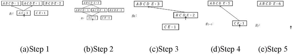
Figure 7 An example of CFSM-AKB algorithm.

Example 6. Figure 7 shows a brief example of the algorithm. Five sequences with their supports are shown in Figure 7(a). We point cursor $c$ to $< A, C >$ at first. Then we find that two sequences are supersequences of $c$ , as stated above, $b_{k_{1}} = < A, B, C, D >$ and $b_{k_{2}} = < A, C, D, E >$ . We merge $c$ to $b_{k_{1}}$ , by invoking FSMerge $(L, b_{k_{1}}, c)$ . Then we invoke FSCombine $(L, b_{k_{2}}, b_{k_{1}})$ to combine $b_{k_{1}}$ and $b_{k_{2}}$ into a new entry containing $< A, B, C, D, E >$ , as shown in Figure 7(b). Since the maximum length is increased from 4 to 5, in Figure 7(c), we move cursor $c$ to the head of $g_{t} = < B, C, D, E >$ . Since there is one sequence $< A, B, C, D, E >$ as a supersequence of $< B, C, D, E >$ , we only invoke FSMerge in this time. In Figure 7(d), since $c$ points to the tail of $g_{j}$ with Lines 15–16, we move $c$ to the head of $g_{j - 1}$ to $< C, E >$ . Then we also invoke FSMerge. Finally in Figure 7(e), the algorithm ends when $c$ points to the tail of $g_{1}$ . We get the generated sequence $< A, B, C, D, E >$ with support 6.

5.2 Properties of CFSM-AKB

In this section, we study the properties of our algorithm including the time complexity and the correctness.

Time Complexity. We consider the upper bound of our algorithms. The worst situation is that the longest length of sequences is always changed after the combination of two entries. Such operation will generate one new entry and delete two in each round. Let $n$ denote the number of all input sequences. We choose a group with at most $l$ entries in each round and the function FSCombine is invoked $n \times l$ times. According to the analysis in Section 4.2.4, the time complexity of function FSCombine is $\max {O (l), O (m)}$ . Consequently, the CFSM-AKB algorithm is polynomial time and requires $\max {O (n l^{2}, O (n l m)}$ arithmetic operations.

Correctness. Since the optimal solution of the problem satisfies three conditions, we will prove the correctness of CFSM-AKB algorithm by showing that its results satisfy these conditions in Lemma 3 and 4.

Lemma 1. In CFSM-AKB algorithm, $\exists b \in g_{j + δ}$ and $\forall d \in g_{j + ε}$ , respectively, where $0 \leq ε < δ \leq l - j$ , $d$ is deleted iff $d . s e q ⊏ b . s e q$ .

Lemma 2. If $d$ is deleted, $d$ is not to be rebuilt.

Proof. We use induction to prove this lemma.

• When $| d . s e q | = 1$ , since $d . s e q$ contains only one element, if it is deleted, there are no subsequences to be combined, but $d$ cannot be rebuild apparently.

• When $\forall e_{i}$ , $| e_{i} . s e q | = l, l < n$ , we suppose that if $e_{i}$ is deleted, $e_{i}$ is not to be rebuilt.

• When $| d . s e q | = n$ , we attempt to prove that if $d$ is deleted, d is not to be rebuilt.

First, since $d$ is deleted, $\exists b$ such that $d . s e q ⊏ b . s e q$ . (Lemma 1) Then, we use contradiction. Suppose that $d$ is rebuilt. In such case, FSCombine $(L, e_{1}, e_{2})$ must be invoked, where $e_{1}$ and $e_{2}$ satisfy following conditions.

• $e_{1} \in g_{j + μ_{1}}, μ_{0} < μ_{1} < ε$ , and

• $e_{2} \in g_{j + μ_{2}}, μ_{0} < μ_{2} < ε$ , and

• $\exists e_{0}$ such that $e_{0} \in g_{j + μ_{0}}, 0 < μ_{0} < ε$ , and

• $e_{0} . s e q ⊏ e_{1} . s e q$ and $e_{0} . s e q ⊏ e_{2} . s e q$ .

In other words, $| e_{1} . s e q | < n$ and $| e_{2} . s e q | < n$ . Nevertheless, since $e_{1} . s e q ⊏ d . s e q$ , $e_{2} . s e q ⊏ d . s e q$ , and $d . s e q ⊏ b . s e q$ , we conclude $e_{1} . s e q ⊏ b . s e q$ , $e_{2} . s e q ⊏ b . s e q$ . Hence, FSMerge $(L, b, e_{1})$ and FSMerge $(L, b, e_{2})$ to delete $e_{1}$ and $e_{2}$ . $e_{1}$ and $e_{2}$ will not be rebuilt, in accordance with the assumption that $\forall e_{i}, | e_{i} . s e q | = l, l < n$ , if $e_{i}$ is deleted, $e_{i}$ are not to be rebuilt. Therefore, $d$ does not exist, either. This is contradict to the assumption that $d$ is rebuilt. Thus, for any $d$ , $| d . s e q | = n$ , if it is deleted, it is not to be rebuilt.

As a result, for any $d$ , if it is deleted, it will not be rebuilt. This lemma holds.

Lemma 3. For the result set $T$ of CFSM-AKB algorithm, both $c o v (T)$ and $\frac{Σ | t_{i} |}{| T |}$ are maximal.

Proof. Firstly, we prove that two claims in this lemma are equivalent.

• Formally, let $S_{T}^{D}$ denote the union of compatible set of all generated rules that $S_{T}^{D} = ⋃_{t_{i} \in T} S_{T}^{D}$ .Accprdomg to the function that $c o v (T) =$ $\frac{| S_{T}^{D} |}{| D |}$ , if we want to maximize $c o v (T)$ , for the same data set $D$ , we should maximize $S_{T}^{D}$ . In other words all sequences in $D$ should be covered by sequences in $T$ . It is impossible that a sequence $s^{'}$ in $D$ but not in $S_{T}^{D}$ is a subsequence of any sequences in $T$ .

• Similarly, according to the function that $\frac{Σ | t_{i} |}{| T |}$ , if we want to maximize it, we should maximize $Σ | t_{i} |$ . Because the combination of two sequences increases the average length, we should ensure that there does not exist two sequences in $T$ satisfy the condition that one is a subsequence of the other. Formally, $\forall t_{v} \in T$ , there does not exist $t_{u} \in t$ such that $t_{u} ⊏ t_{v}$ .

Therefore, all we need is to prove that during the algorithm such $s^{'}$ and $t_{v}$ do not exist. We set $t_{i}$ and $t_{v}$ correspond to $b . s e q$ , and $s^{'}$ and $t_{u}$ correspond to $d . s e q$ . Thus, two claims are equivalent.

According to Lemma 1 and $d . s e q ⊏ b . s e q$ , $d$ is deleted. According to Lemma 2, $d$ is not to be built. As a result, in $T$ , there does not exists $d$ such that $d . s e q ⊏ b . s e q$ . This lemma holds.

Lemma 4. The frequency of each sequence generated by CFSM-AKB algorithm is over a threshold. Formally, for the result set $T$ of CFSM-AKB algorithm, $\forall t_{i} \in T, | S_{t_{i}}^{D} | \geq ϵ_{f}$ .

Proof. In Algorithm 6 with Line 20, only sequences whose supports are over the predetermined threshold $ϵ_{f}$ are output. Thus, this lemma holds.

According to these lemmas, the following theorem shows the correctness of CFSM-AKB algorithm.

Theorem 1. The CFSM-AKB algorithm is correct because of the output of that, $T$ , satisfies three following claims.

• $c o v (T)$ is maximal, and

• $\frac{Σ | t_{i} |}{| T |}$ is maximal, and

• $\forall t_{i} \in T, | S_{t_{i}}^{D} | \geq ϵ_{f} .$

Proof. According to Lemma 3 and 4, $\forall T$ , we have $\forall t_{i} \in T, | S_{t_{i}}^{D} | \geq ϵ_{f}$ , $c o v (T)$ and $\frac{Σ | t_{i} |}{| T |}$ reach their maximum value, respectively. Therefore, CFSM-AKB algorithm is correct for achieving the goal of problem.

6 Experiments and Analyses

To verify the performance of the proposed approach, we conduct extensive experiments on both real and synthetic data. We perform the experiments on a PC machine with 3.1GHz Intel(R) Core(TM) CPU and 8GB main memory, running Microsoft Windows 7. All algorithms are implemented in C language in Microsoft Visual Studio 2013.

To evaluate the performance comprehensively, we test three aspects of our algorithms. During the experiments, default parameters are $α = 0.2$ and $p = 0.005$ .

6.1 Effectiveness

We use the BMSWebView2 dataset [31] used in KDD-CUP competition to test the effectiveness of the propose approach, since such data set contains sequences of click-stream data and such sequence could construct a graph for simple path traversal patterns. This data set contains 77,512 records. We use 65,000 records as the training set, and others are used as the test set. Note that we use $e_{c o v} = \frac{⋃_{t_{i} \in T} S_{t_{i}}^{D}}{| D_{t e s t} |}$ as measure of the effectiveness of the approach.

Comparisons. We conduct three experiments for comparisons. The first one is to compare the effectiveness of the proposed algorithm with two frequent sequence discovery algorithms, PrefixSpan [24] and RuleGen [41]. Even though some other approaches have been proposed such as SPADE [41], SPAM [2], and LAPIN [39], they share the same result with PrefixSpan. Meantime, PrefixSpan have a relative better performance on large data set. RuleGen is a classic algorithm on frequent sequences mining problems, whose purpose is similar to CFSM-AKB. To ensure the fairness of the comparison, we tune the parameters of PrefixSpan and RuleGen, and pick two groups of parameters for each algorithm. These parameters make the algorithm achieve high coverage and could accomplish the computation in a reasonable time (within 2 hours).

Table 1 Compared with PrefixSpan and RuleGen

Algorithm	Parameters	Coverage	Amount
CFSM-AKB	$α = 0.2, p = 0.005, m_{s} = 10$	0.8320	1008
PrefixSpan	$m_{s} = 0.001$	0.0713	30586
PrefixSpan	$m_{s} = 0.0001$	0.2622	8597444
RuleGen	$m_{s} = 100, m_{c} = 0.6$	0.0231	98744
RuleGen	$m_{s} = 50, m_{c} = 0.6$	0.0424	3343536

The experimental results are shown in Table 1, where $m_{s}$ and $m_{c}$ are minimum support and minimum confidence, respectively. To show the benefits of our approach, we also report the number of discovered sequences shown in the Amount column. From the experimental results, we find that our algorithm achieves the highest coverage with relative few sequences. It shows that our algorithm outperforms existing algorithms in effectiveness significantly.

The Effect of Parameters. In this section we test the impact of the parameters $p$ and $α$ on the effectiveness of the proposed algorithm. The experimental results are shown in Figure 8. From the results, it is observed that when $p$ goes higher, which implies more precise prediction, the coverage also increases. Another observation is that if $α$ goes higher, the coverage increases due to the decline of error tolerance. These observations show that our design goal is achieved with these two parameters.

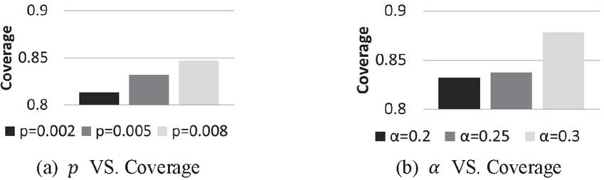
Figure 8 Coverage associated with different parameters.

The Effect of Training Set. In this part, we generate synthetic datasets according to the approach introduced in [3]. Intuitively, the properties of the training dataset can also influence the results. Thus, we test the effect of the properties of training sets on the effectiveness. We consider three parameters of the training sets, total entries (E), max rule sequence length (L) and number of elements (I). We generate six datasets to examine the effect of different datasets. For each data set, 80 percent of data are regarded as the training data, other 20 percent as the test data.

The experimental results are shown in Figure 9(a), where E100L20I100 means there are total 100k entries, max rule sequence length is 20, containing 100 elements, and so on. The y-axis is the coverage.

From the experimental results, we have three observations. First, with fixed $L$ and $I$ , a larger $E$ leads to a better coverage. It is because that more rules could be discovered from a larger training sets. Second, with a fixed $E$ , when $L$ and $I$ increase, the coverage decreases. The reason is that more elements lead to more complex rules and make the rules difficult to discover. Third, even though the coverage decreases with the increasing $L$ and $I$ , we could still increase the coverage by enlarging the size of training data set.

Figure 9 Pruning strategy tested with different parameters.

6.2 Efficiency

We test the efficiency of CFSM-AKB Algorithm on synthetic data set generated in the same way as in Section 6.1.3. We vary $E$ from 5k to 100k to test the efficiency on training set with various data sizes. In the experiments, we set $L = 20$ and $I = 100$ . The experimental results are shown in Figure 9(b), where the x-axis is the size of total entries of a dataset and y-axis is the rule discovery time on the data set. From the experimental results, the running time is around linear with the number of entries, which agrees with the time complexity in Section 5.2.

6.3 Effectiveness of Pruning Strategy

Since in FSCombine algorithm, the combination of two long sequences results in error in high probability, we test the probability that two sequences with different lengths can be combined according to our pruning strategy. We test the results on different $p$ and $α$ . Dataset and the parameters are the same as those in Section 6.1.

Figure 10 Pruning strategy tested with different parameters.

Figure 10 shows the restraint effect of combination of two sequences, where x-axis indicates the length of long sequence, and y-axis that of short one. Each line in each figure shows the maximum length of short sequence that can be combined with long sequences with various lengths. The experimental results are shown in Figures 10(a) and 10(b) with different $p$ and $α$ , respectively. From the experimental results, the probability that two sequences with different lengths can be combined increases with the decline of $p$ but with the increasing of $α$ . From this observation, we conclude that $p$ and $α$ could control the lengths of sequences involved in the combination successfully. It demonstrates the effectiveness of the proposed pruning strategy.

6.4 Summary

The following conclusions are drawn from the experimental findings. From an acyclic knowledge base, the suggested method may extract valuable frequent sequences. The suggested method considerably surpasses current alternatives in terms of effectiveness. The suggested method is fast and can handle a high number of training sets. The pruning method provided is successful. The length of the sequences involved in the combination might be adjusted using the two parameters.

7 Related Work

The original work of sequential pattern mining is to acquire all sequential patterns with a predefined support from a database of sequences [32], where classic works are GSP [32], SPADE [41], PrefixSpan [24], Spam [2], Lapin-Spam [39]. All of them input the same training set and parameters and return the same set of frequent sequential patterns. There are also tons of sequential patterns mining algorithms designed under diverse background recently, such as Skopus [25], uWSequence [28], WoMine [4], UNB [35], etc. The problem definition of our work is different from these works because we aim at mining simple path traversal patterns from a knowledge graph. As a result, they are ineffective to directly apply them to our problem.

There is also a body of work on sub-graph mining. They are concerned with acquiring frequent sub-graphs in a graph, such as gSpan [38], Spin [14], Leap [37], ATW-gSpan [16], AW-gSpan [16], UBW-gSpan [16], DistGraph [34], MuGraM [15]. Additionally, there are data mining for path traversal patterns under different circumstances, especially on World Wide Web [5, 21]. However, their goals are different from ours. They lack the consideration of Coverage.

Another related literature is on the topic of knowledge graph mining. One of popular researches is utilizing data mining for developing and maintaining a knowledge graph [11, 17, 30], which are not of our concern. Fortunately, several researches are involving data mining on the knowledge graph in recent years, such as rule mining [8, 10, 27], mining outliers [22], mining cardinality [20], mining conditional keys [33], mining substructures [7], mining user behaviour information [29]. Diverse data mining tasks are springing up on account of emerging researches of knowledge graph. To our best knowledge, our work is the first study of mining simple path traversal patterns on it.

8 Conclusions

In this paper, we have solved the problem of simple path traversal patterns mining in knowledge base. Our model is a special frequent sequence mining problem with consideration of coverage. To tackle this problem, we propose an algorithm based on sequence combination. To increase the efficiency and effectiveness, we develop a suitable data structure and algorithms for sequence combination as well as pruning strategies. We prove algorithm proposed is correct. Extensive experiments demonstrate that the proposed approach could find useful frequent sequences efficiently and effectively. The further works include mining different paths in knowledge graph, mining frequent patterns in knowledge graph, and other data mining problems in knowledge graph. We believe that studying data mining in the context of knowledge graphs will lead to exciting new research.

Acknowledgements

This paper was supported by NSFC grant U1866602. CCF-Huawei Database System Innovation Research Plan CCF-HuaweiDBIR2020007B.

References

[1] Augenstein, I., Das, M., Riedel, S., Vikraman, L. and McCallum, A., 2017. Semeval 2017 task 10: Scienceie-extracting keyphrases and relations from scientific publications. arXiv preprint arXiv:1704.02853.

[2] Ayres, J., Flannick, J., Gehrke, J. and Yiu, T., 2002, July. Sequential pattern mining using a bitmap representation. In Proceedings of the eighth ACM SIGKDD international conference on Knowledge discovery and data mining (pp. 429–435).

[3] Ashwin Balani. Another alternative for generating synthetic sequences databases. http://philippe-fournier-viger.com/spmf/SequentialPatternGenerator.m, 2015.

[4] Chapela-Campa, D., Mucientes, M. and Lama, M., 2019. Mining frequent patterns in process models. Information Sciences, 472, pp. 235–257.

[5] Chen, M.S., Park, J.S. and Yu, P.S., 1998. Efficient data mining for path traversal patterns. IEEE Transactions on knowledge and data engineering, 10(2), pp. 209–221.

[6] Cormen, T.H., Leiserson, C.E., Rivest, R.L. and Stein, C., 2009. Introduction to algorithms. MIT press.

[7] Costa, J.D.J., Bernardini, F., Artigas, D. and Viterbo, J., 2019. Mining direct acyclic graphs to find frequent substructures—an experimental analysis on educational data. Information Sciences, 482, pp. 266–278.

[8] Galárraga, L. and Suchanek, F., 2016. Rule Mining in Knowledge Bases (Doctoral dissertation, Thèse, Spécialité “Informatique”, TELECOM ParisTech).

[9] Deshpande, O., Lamba, D.S., Tourn, M., Das, S., Subramaniam, S., Rajaraman, A., Harinarayan, V. and Doan, A., 2013, June. Building, maintaining, and using knowledge bases: a report from the trenches. In Proceedings of the 2013 ACM SIGMOD International Conference on Management of Data (pp. 1209–1220).

[10] Galárraga, L., 2014, November. Applications of rule mining in knowledge bases. In Proceedings of the 7th Workshop on Ph. D Students (pp. 45-49).

[11] Galárraga, L.A., Preda, N. and Suchanek, F.M., 2013, October. Mining rules to align knowledge bases. In Proceedings of the 2013 workshop on Automated knowledge base construction (pp. 43–48).

[12] Gao, J., Qiu, H., Jiang, X., Wang, T. and Yang, D., 2010, October. Fast top-k simple shortest paths discovery in graphs. In Proceedings of the 19th ACM international conference on Information and knowledge management (pp. 509–518).

[13] Hershberger, J., Maxel, M. and Suri, S., 2007. Finding the k shortest simple paths: A new algorithm and its implementation. ACM Transactions on Algorithms (TALG), 3(4), pp. 45–es.

[14] Huan, J., Wang, W., Prins, J. and Yang, J., 2004, August. Spin: mining maximal frequent subgraphs from graph databases. In Proceedings of the tenth ACM SIGKDD international conference on Knowledge discovery and data mining (pp. 581–586).

[15] Ingalalli, V., Ienco, D. and Poncelet, P., 2018. Mining frequent subgraphs in multigraphs. Information Sciences, 451, pp. 50–66.

[16] Jiang, C., Coenen, F. and Zito, M., 2010, August. Frequent sub-graph mining on edge weighted graphs. In International Conference on Data Warehousing and Knowledge Discovery (pp. 77–88). Springer, Berlin, Heidelberg.

[17] Li, X., Taheri, A., Tu, L. and Gimpel, K., 2016, August. Commonsense knowledge base completion. In Proceedings of the 54th Annual Meeting of the Association for Computational Linguistics (Volume 1: Long Papers) (pp. 1445–1455).

[18] Liang, J., Xiao, Y., Zhang, Y., Hwang, S.W. and Wang, H., 2017, February. Graph-based wrong isa relation detection in a large-scale lexical taxonomy. In Thirty-First AAAI Conference on Artificial Intelligence.

[19] Luo, T. and Yu, J., 2019. Friends along supply chain and relationship-specific investments. Review of Quantitative Finance and Accounting, 53(3), pp. 895–931.

[20] Muñoz, E. and Nickles, M., 2017, August. Mining cardinalities from knowledge bases. In International Conference on Database and Expert Systems Applications (pp. 447–462). Springer, Cham.

[21] Nanopoulos, A. and Manolopoulos, Y., 2001. Mining patterns from graph traversals. Data & Knowledge Engineering, 37(3), pp. 243–266.

[22] Nowak-Brzeziñska, A., 2017, July. Outlier mining in rule-based knowledge bases. In 2017 IEEE International Conference on INnovations in Intelligent SysTems and Applications (INISTA) (pp. 391–396). IEEE.

[23] Oswald, C., Kumar, I.A., Avinash, J. and Sivaselvan, B., 2017, December. A graph-based frequent sequence mining approach to text compression. In International Conference on Mining Intelligence and Knowledge Exploration (pp. 371–380). Springer, Cham.

[24] Han, J., Pei, J., Mortazavi-Asl, B., Pinto, H., Chen, Q., Dayal, U. and Hsu, M., 2001, April. Prefixspan: Mining sequential patterns efficiently by prefix-projected pattern growth. In proceedings of the 17th international conference on data engineering (pp. 215–224). IEEE Washington, DC, USA.

[25] Petitjean, F., Li, T., Tatti, N. and Webb, G.I., 2016. Skopus: Mining top-k sequential patterns under leverage. Data Mining and Knowledge Discovery, 30(5), pp. 1086–1111.

[26] Poole, D.L. and Mackworth, A.K., 2010. Artificial Intelligence: foundations of computational agents. Cambridge University Press.

[27] Pujara, J. and Singh, S., 2018, February. Mining knowledge graphs from text. In Proceedings of the Eleventh ACM International Conference on Web Search and Data Mining (pp. 789–790).

[28] Rahman, M.M., Ahmed, C.F. and Leung, C.K.S., 2019. Mining weighted frequent sequences in uncertain databases. Information Sciences, 479, pp. 76–100.

[29] Shang, F., Ding, Q., Du, R., Cao, M. and Chen, H., 2021. Construction and Application of the User Behavior Knowledge Graph in Software Platforms. J. Web Eng., 20(2), pp. 387–412.

[30] Shin, J., Wu, S., Wang, F., De Sa, C., Zhang, C. and Ré, C., 2015, July. Incremental knowledge base construction using deepdive. In Proceedings of the VLDB Endowment International Conference on Very Large Data Bases (Vol. 8, No. 11, p. 1310). NIH Public Access.

[31] Blue Martini Software. Bmswebview2 (gazelle) dataset. http://www.kdd.org/sites/default/files/kddcup/site/2000/files/KDDCup2000.zip

[32] Srikant, R. and Agrawal, R., 1996, March. Mining sequential patterns: Generalizations and performance improvements. In International conference on extending database technology (pp. 1–17). Springer, Berlin, Heidelberg.

[33] Symeonidou, D., Galárraga, L., Pernelle, N., Saïs, F. and Suchanek, F., 2017, October. Vickey: Mining conditional keys on knowledge bases. In International Semantic Web Conference (pp. 661–677). Springer, Cham.

[34] Talukder, N. and Zaki, M.J., 2016. A distributed approach for graph mining in massive networks. Data Mining and Knowledge Discovery, 30(5), pp. 1024–1052.

[35] Ting, I.H., Kimble, C. and Kudenko, D., 2009. Finding unexpected navigation behaviour in clickstream data for website design improvement. Journal of Web Engineering, 8(1), p. 71.

[36] Wu, W., Li, H., Wang, H. and Zhu, K.Q., 2012, May. Probase: A probabilistic taxonomy for text understanding. In Proceedings of the 2012 ACM SIGMOD International Conference on Management of Data (pp. 481–492).

[37] Yan, X., Cheng, H., Han, J. and Yu, P.S., 2008, June. Mining significant graph patterns by leap search. In Proceedings of the 2008 ACM SIGMOD international conference on Management of data (pp. 433–444).

[38] Yan, X. and Han, J., 2002, December. gspan: Graph-based substructure pattern mining. In 2002 IEEE International Conference on Data Mining, 2002. Proceedings. (pp. 721–724). IEEE.

[39] Yang, Z., Wang, Y. and Kitsuregawa, M., 2007, April. LAPIN: effective sequential pattern mining algorithms by last position induction for dense databases. In International Conference on Database systems for advanced applications (pp. 1020–1023). Springer, Berlin, Heidelberg.

[40] Yen, J.Y., 1971. Finding the k shortest loopless paths in a network. management Science, 17(11), pp. 712–716.

[41] Zaki, M.J., 2001. SPADE: An efficient algorithm for mining frequent sequences. Machine learning, 42(1), pp. 31–60.

Biographies

Feng Xiong received the BEng degree in computer science and technology at Harbin Institute of Technology, China, in 2015. He is now working toward the PhD degree in computer science at Harbin Institute of Technology, China. His research interests include knowledge base, data quality management, data mining, and big data.

Hongzhi Wang is a Professor and doctoral supervisor at Harbin Institute of Technology, ACM member. His research area is data management, including data quality and graph management. He is a recipient of the outstanding dissertation award of CCF and Microsoft Fellow.