Air Quality Prediction Based on Wavelet Analysis and Machine Learning
Jun Duan1 and Qi Ren2,*
1School of Economics & Management, Chongqing Normal University, Chongqing 401331, China
2Institute of Intelligent Engineering, Chongqing City Management College, Chongqing 401331, China
E-mail: Duan@cqnu.edu.cn; renqi666999@126.com
*Corresponding Author
Received 28 October 2021; Accepted 15 January 2022; Publication 28 December 2022
Abstract
This thesis takes the historical weather time series of Chongqing as experimental samples. Firstly, this thesis uses wavelet transform to organize the data, and then divides the sample data into training and test sets to verify the accuracy of the evaluation of the Naive Bayes Model. Secondly, the Naive Bayes Model is compared with currently used machine learning models such as SVM, XGBoost, bagging, and random forest. Finally, the results show that the Naive Bayes Model has high stability and accuracy for the air quality assessment of Chongqing, and it can be applied to the evaluation of urban ambient air quality.
Keywords: Machine learning, weather quality, prediction.
1 Introduction
With the rapid development of social economy, it looks beyond dispute that the issue about the air quality has aroused universal attention. The air quality is seriously degraded, and the smog phenomenon is frequent. The serious air pollution in winter and spring leads to people’s travel difficulties or sudden illnesses, which has attracted great attention from the country. To further interpret the trend of air changes and understand the pollution of air quality, it is necessary to predict the air quality index in a timely and accurate manner. When it is predicted that heavy pollution will occur, countermeasures like reducing pollutant emissions should be taken decisively. Consequently, scientific and accurate prediction of changes in air quality and effective evaluation of air quality are of great guiding significance for improving air pollution, promoting urban environmental construction, and guiding people’s production and lifestyle. Similarly, the air quality evaluation index is a value that combines the concentrations of several air pollutants routinely monitored according to environmental quality standards and the impact of various pollutants on human health, ecology, and the environment, which can intuitively reflect the air degree of pollution. A Bayesian model is a mathematical model wherein possibility has been used to portray all ambiguity inside the model, such as ambiguity about outcome and also lack of certainty about the model’s input. 10-fold cross validation would replicate the suitable procedure 10 times, for each fit conducted on a training dataset comprised of 90 percentage points of an overall training set picked at random, with residual 10 percentage points using it as a verification hold out set. Here, the air quality is predicted by using machin learning technique. Where, this type of prediction system helps to develop the urban environments also, with its accurate outcome. It produces the accurate result. Therefore, the establishment of a high-precision model to predict the future air quality index, whether it is for the prevention of air pollution or the improvement of air quality, can provide good theoretical guidance.
Scholars at home and abroad have done a lot of research on air quality assessment methods. It can be summarized into two types. One is traditional mathematical model evaluation methods such as fuzzy evaluation method, rough set, multiple linear regression, time series, etc. The other is machine learning method.
2 Related Work
At present, there have been many traditional methods of evaluating air quality at home and abroad. Onkal-Engin [1] evaluated the air quality of Istanbul using fuzzy comprehensive evaluation method, Chang S C and Lee [2] analyzed the air quality in Taiwan Province of China from 1994 to 2003 by using principal component analysis. Fuzzy set theory underscores the fuzzy evaluation method. It is used to encapsulate the unknowns that arise in a framework. As noted previously, the mechanisms involved in usability testing encompass essentially fuzzified, ambiguous, dynamic, and transforming information. This fuzzy evaluation model has advantages over conventional methods and can help usability testing in 2 directions: The fuzzy assessment process, which is premised on fuzzy sets, is an attractive means of designing the ambiguity or lack of accuracy that emerges from human cognition. This is neither arbitrary nor randomness. Zhang et al. [3] used AHP to analyze the air quality of Qingdao from 2004 to 2013, and it equally revealed that the air quality of Qingdao in the past 10 years had been in line with the National Air Quality Standard II. Li [4] introduced the concepts of residual fractional index and supplementary composite index, and proposed a new method for synthetically calculating the comprehensive index of atmospheric environmental quality using residual index. Li [5] and others established a multiple regression model of air quality influencing factors in Beijing from 1999 to 2009, and obtained the conclusions of the air quality evaluation results of multiple factors, thus further obtaining the urban green space coverage rate and population size have a significant impact on Beijing’s air quality. Multiple regression analysis enables users to examine the strength of relationship between a results as well as several predictors, and the significance of each predictor to the connection, commonly with the impact of other predictor variables statistical significant completely eradicated [6, 7]. The intrinsic mapping function is used in proposed model top find the relationship between the various pollutants in urban air and air quality level. Zhang et al. [8] evaluated the air quality in Golmud based on the matter-element analysis theory, and the results were consistent with the status of air quality in Golmud.
Scholars and experts at home and abroad have also conducted in-depth research on the use of to solve environmental impacts, and have proposed many efficient and concise machine learning algorithms [11]. In the data-based machine learning algorithm, the neural network model has a good prediction effect on studying air quality prediction [9–12]. Wang [13], Chen, etc. [14] used decision tree algorithm to build an air quality evaluation system, and use historical data of air pollutants and quality levels to establish an intelligent evaluation model for air level discrimination [14]. Guo et al. [15, 16], Hu et al. [17, 18] used support vector machine algorithm to predict air quality. Currently, machine learning (ML) in artificial intelligence (AI) is the most popular implementation method, while deep learning (DL) is a branch of machine learning (ML) and one of the most popular machine learnings (ML) [19, 20]. Deep learning theory is expanding rapidly. Considering that air quality monitoring data belongs to time series data, by referring to related literature [21], the Naive Bayes Model has been widely used in time series prediction, and achieved good prediction results.
3 Econometric Framework
This section briefly presents the DWT and SVR approaches. Both approaches on their own are well established in the literature, and applications in this context relying on standard specifications [22]. To classifier and categorise the failure pattern in above power line, a difference relay selection generic term referring on the Discrete wavelet transform approach is used. The system starts with signals derived instantaneously both from end points of the power line and filtered through DWT to acquire Spectral Energy. The expansion for SVR is Support Vector Regression. Support Vector Regression is a supervised learning model for forecasting distinct values. The same important framework Support Vector Regression because it does SVMs. SVR’s basic principle is to find the best fit line [23]. Therefore, I only provide an intuitive introduction. In general, estimation follows a two-step procedure where the DWT is firstly used to create an extended database that includes all decomposition of the original predictor series; then, in a second step, this database is used as the input for the SVR in order to identify the most important trend components for forecasting gold returns. Since the evaluation includes a true out-of-sample forecasting exercise, the procedure is replicated in every period of time in which new data becomes available [24].
3.1 Discrete Wavelet Transform
3.1.1 Wavelet transform
Wavelets are function that is oscillatory with ability to attenuate to zero rapidly. Wireless transceivers usually employ bandpass filters. The basic task of such a filtration system in a transceiver is to constrain the frequency band of the output voltage to the transmitting band. This guarantees that the transceiver doesn’t really interfere with the other terminals [25]. Wavelet transform refers to band-pass filter to filter signals at different scales. Given are space for all squared integration functions, Fourier is transformed into . When meet the condition:
| (1) |
Then is a wavelet mother function. Of which, should meet . That is. And then has band pass property.
A wavelet function is formed by translation and scaling of the wavelet mother function , as shown in formula (2) below:
| (2) |
are sub-wavelets; is the scale parameter, and is the time parameter, which reflects the translation of wavelet in time.
Wavelet transform of signal is defined as:
| (3) |
In formula (3), is complex conjugate function of . are wavelet coefficients at different locations and scales. Since the variables in formula are continuous, the upper formula (3) is called continuous wavelet transform. The complex conjugate is used to justify complex numbers and to determine the magnitude of a complicated number’s polar form. As actual financial data are generally discrete, the parameter are discrete in practice, but this discretization is not only for time variable . Discrete form is as follows:
| (4) |
In formula (4), N is discrete point, and is sampling interval. can reflect the characteristics of time parameter and scale parameter . And when the is small, it has low resolution in frequency domain, and high resolution in time domain; As the gets bigger, it has high resolution in frequency domain, and low resolution in time domain. Therefore, wavelet transform can localize time-series time frequency, and analyze the local.
Wavelet Denoising Method
Noise could interfere with effective information that might exist in the data so that it is very important to obtain effective information from the research data purposefully to remove the useless and interfering noise. Noise is considered in communication research and pattern recognition as anything else that tries to interfere with the process of communication among a speaker and a viewers. Noise is both external and internal and it can interrupt interaction anywhere at point. In the wavelet domain, the corresponding coefficients of the effective signal are very large while noise corresponds to small coefficients. The coefficients corresponding to noise in wavelet domain still satisfy the Gaussian white noise distribution, which can be evaluated by wavelet coefficients or raw signals, to eliminate threshold value of noise in wavelet domain. At present, the common thresholds value includes fixed threshold method, minimax threshold method as well as heuristic method. Fixed Thresholding Methods is the attribute was derived from the Color space, that also explains a paint pixel as a proportion of Hue, Density, and Valuation. Concentration helps the reader understand a color combinations “lightness,” to simple colour needing a concentration value of 0 and pure mixed race needing a maximum point of just one.
After threshold selection method appearing, the threshold function is introduced to filter the wavelet coefficients with noise. A threshold function is a Boolean process that describes whether value equal opportunity of its input data has exceeded a certain limit. A threshold gate is a gadget that enforces such logic. At present, we mainly use soft threshold and hard threshold function, which was proposed by Donoho in 1995.
Hard threshold denoising method. When the absolute value of wavelet coefficients is less than the given threshold, it is set as 0; Conversely, it remains the same, i.e.:
| (5) |
Soft threshold denoising method. When the absolute value of wavelet coefficients is less than a given threshold, it is set as 0. Conversely, the threshold value is subtracted, i.e.:
| (6) |
Hard threshold function is superior to soft threshold method in mean square error sense, but the signal creates an extra shock, a jump point, unable to smooth the original signal well. A soft threshold is a data pre-processing tool that lessens the Backstory in a picture by lowering Rasterization with intensity values less than that of the threshold level. These thresholded voxels become much more translucent during visualisation. All Framelet coefficients greater than just a given threshold are maintained in a hard threshold, and the remainder correlations are reduced to 0. The wavelet coefficients obtained by soft threshold function have good continuity to make the overall signal smoother without obvious jump point. However, the signal will be compressed to produce a certain error. Therefore, in practice, it needs ceaseless attempts for selecting better processing method to improve the estimation accuracy.
3.2 Naive Bayes
Naive Bayes, a probabilistic classification method, is supported by solid mathematical theory. And it has the characteristics of high classification accuracy, simple implementation, insensitive to missing data and less estimation parameters. In theory, compared with other classification algorithms, its error rate is minimal, but it has a premise that is requirement for feature independence. That is, each characteristic variable of the item to be classified is independent, where there is less actual situation that can fully satisfy this condition so that it has a slight effect on the accuracy of the classification.
The principle of Naive Bayes is that: given , is sample to be classified, is characteristic variables of , and are independent from each other, . Given , is collection of categories and there is a total of categories. To calculate the probability of each category under the condition of appearing and the category with the highest probability is the final category of , i.e.:
| (7) |
is the final category of . When calculating conditional probability, Bayes formula and total probability formula needed, such as formula (8) and formula (9).
| (8) | ||
| (9) |
Of which, is obtained from proportion of sample groups and is obtained from conditional probability of characteristic variables appearing in the sample set.
3.3 Model Performance Evaluation
The validity of all models is evaluated by accuracy and root mean square error in this paper. And the accuracy of each category can also be estimated by formula TP/(TPFP), where TP indicates the number of correct estimates while FP indicates the number of times an error has been estimated.
| (10) |
In the formula, n indicates the number of observations, represents the predicted value and represents the observed data. The exact range is from 0 to 1, where 1 represents the perfect fit of observations and predictions. When the exact value is 0, this model is invalid. The root mean square error is the evaluation of the sample size error, indicating the difference between the observed and predicted values. Hence, the RMSE should be 0 when the observations fit perfectly to the predicted values.
Area under ROC curve is widely used to measure the performance of regulatory classification rules but the simple form applies only to two categories of situations. Receiver operating characteristic curves make a comparison responsiveness vs selectivity for the ability to anticipate a dichotomous result across such a value range. Another measurement for test scores is the area under ROC curve. In this paper, the definition is extended to more than two categories by pairwise average comparison.
Given that multiple categories are labeled as 1, 2, …, c(c 2), the known classification rules give us estimated value of each probability when each test value belongs to the corresponding classification. For any pair of numbers at i and j level, or can be used to measure the value of A. Therefore, is defined as arbitrary extraction number at j levels which the probability of belonging to the j level is less than the probability of random sampling to that number at the i level. Above classification rules in the separation of c levels of the calculation process is the same as the average algorithm for all levels of classification.
| (11) |
Range of M value is from 0 to 1, where a value of 1 indicates that the estimated data is fully fit to the actual data.
4 Experiment and Results Analysis
4.1 Data Preparation
This study uses several predictive techniques to forecast the air quality index (AQI) for the year 2020 and selects the historical measurement data from 2015 to 2019 to train the model. Government agencies use an Air Quality Index to inform the people how contaminated the air is here and how contaminated it is anticipated to be become. Pollutant emissions, transit and diffusion of toxins by wind gusts, reactive species between many reactionary gaseous pollutants, and removal processes including such downpours and outer layer deposition are being used to predict quality of the air. The wavelet was used as a pre-processing tool to decompose the original time series.
4.2 Selection of Experimental Sample Data
Although the air quality in Chongqing has improved, there is still space for improvement. Exploring reasonable and scientific urban air quality assessment methods is capable of finding the law of air quality change in Chongqing, which has great scientific significance for controlling its air pollution. The data used in the experiments in this thesis comes from the Chongqing Municipal Air Quality Monitoring Bureau and the Chongqing Monitoring Center, which release daily air quality monitoring information. The sample data set of the experiment is the daily air quality data of Shanghai from January 1, 2015 to May 24, 2020. There were a total of 1971 sample data. Table 1 indicates some examples of air quality data in Chongqing. The training sample data set of the experiment was randomly sampled with a total of 1576 sample data, accounting for 80% of the total sample. The remaining sample data is the test sample data set, which accounts for 20% of the total sample data. In the experiment, the six main air pollutants CO, O, N0, S0, PM 10, PM 2.5 were used as the characteristic variables for decision-making in the machine learning algorithm model. Finally, the evaluation results of urban air quality are used as the classification results of the machine learning algorithm model, that is to say, six grades of excellent, good, light pollution, moderate pollution, heavy pollution and extremely severe pollution are used as the six classification categories of the algorithm.
Table 1 Part of sample data of air quality in chongqing
| Air Pollutants | |||||||
| Date | PM2.5 | PM10 | SO | CO | NO | O3 | Quality Grade |
| 2019/5/11 | 56 | 94 | 9 | 1 | 53 | 168 | Light Pollution |
| 2019/6/3 | 38 | 88 | 10 | 0.9 | 55 | 218 | Moderate Pollution |
| 2019/7/1 | 40 | 68 | 7 | 1 | 44 | 223 | Moderate Pollution |
| 2019/8/12 | 26 | 55 | 8 | 0.8 | 44 | 277 | Heavy Pollution |
| 2019/9/19 | 13 | 21 | 5 | 0.8 | 28 | 32 | Excellent |
| 2019/10/22 | 12 | 17 | 5 | 0.8 | 30 | 18 | Excellent |
| 2019/11/24 | 24 | 31 | 6 | 0.7 | 30 | 23 | Excellent |
| 2019/12/9 | 98 | 138 | 12 | 1.3 | 67 | 36 | Light Pollution |
| 2020/1/3 | 82 | 124 | 12 | 1.1 | 62 | 28 | Light Pollution |
| 2020/2/8 | 41 | 51 | 6 | 0.8 | 23 | 34 | Good |
| 2020/3/5 | 26 | 37 | 7 | 0.7 | 28 | 50 | Excellent |
| 2020/4/7 | 37 | 64 | 8 | 1 | 54 | 87 | Good |
4.3 Empirical Results
4.3.1 Wavelet transform of data
When processing time series data, db wavelet or sym wavelet is often selected as the wavelet base. The sym wavelet with better symmetry is the nearly symmetric orthogonal wavelet function of db wavelet. In addition, the more wavelet decomposition layers, the better the stationarity of the detail signal and the approximate signal, but this will lead to a greater error in the decomposition process, so all layers must be appropriate. Thus, this paper firstly uses the sym4 wavelet basis to decompose the time series into four layers to reconstruct the time series data and improve the generalization ability of the prediction model. The trend of the reconstructed time series data is shown in the figure below. It can be seen that the time series data after wavelet reconstruction can effectively smooth the original data and retain its approximate signal, for it is theoretically feasible to establish a prediction model based on this data. Each graph represents the variable wavelet decomposition of air prediction. It illustrates the various wavelength of air quality prediction system. It has reconstructed time series information theoretical manner. It can be seen that the time series after wavelet reconstruction could indeed successfully smooth the actual information whereas retaining its estimated signal, suggesting that a predictive algorithm relying on this data is sustain positive.
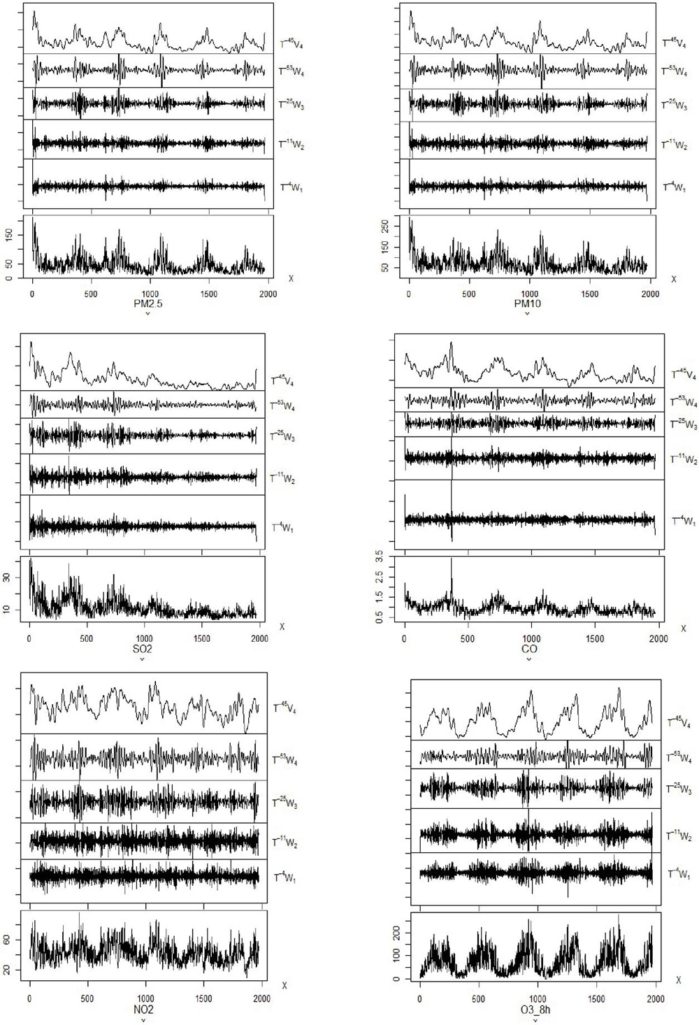
Figure 1 Variable wavelet decomposition diagram.
Compare Multiple Machine Learning Evaluation Models and Analyze Experimental Results.
The evaluation model is constructed by using commonly used algorithms such as SVM, XGBoost, bagging, and random forest. Compared with Naive Bayes Model, a 10-fold cross-validation method is used to verify the evaluation performance. The experimental results are shown in Tables 2 and 3 (the accuracy of the five models on the air quality evaluation of Chongqing).
Table 2 The training results comparison of wavelet transform (the time lagging one period)
| Category Accuracy (P) (%) | ||||||||
| Accuracy | Light | Moderate | Heavy | |||||
| Model | (%) | RMSE | M | Excellent | Good | Pollution | Pollution | Pollution |
| Random forest | 100 | 0.00 | 1 | 100 | 100 | 100 | 100 | 100 |
| Decision tree | 60.88 | 0.75 | 0.52 | 11.79 | 97.86 | 0 | 0 | 0 |
| SVM | 59.49 | 0.75 | 0.50 | 0 | 100 | 0 | 0 | 0 |
| bagging | 100 | 0.00 | 1 | 100 | 100 | 100 | 100 | 100 |
| XGBoost | 85.71 | 0.38 | 0.68 | 68.82 | 99.35 | 67.12 | 44.44 | 33.33 |
| Naive Bayes | 95.93 | 0.52 | 0.91 | 91.57 | 98.39 | 95.49 | 86.67 | 80 |
Table 3 The forecast results comparison of wavelet transform (the time lagging one period)
| Category Accuracy (P) (%) | ||||||||
| Accuracy | Light | Moderate | Heavy | |||||
| Model | (%) | RMSE | M | Excellent | Good | Pollution | Pollution | Pollution |
| Random forest | 61.32 | 0.69 | 0.67 | 17.77 | 94.44 | 3.63 | 0 | 66.67 |
| Decision tree | 59.28 | 0.74 | 0.52 | 10 | 95.72 | 0 | 0 | 0 |
| SVM | 59.54 | 0.74 | 0.50 | 0 | 100 | 0 | 0 | 0 |
| bagging | 62.45 | 0.73 | 0.59 | 21.11 | 90.59 | 3.63 | 0 | 0 |
| XGBoost | 54.70 | 0.77 | 0.63 | 8.88 | 85.89 | 10.91 | 0 | 0 |
| Naive Bayes | 95.42 | 0.55 | 0.91 | 91.11 | 98.29 | 96.36 | 63.63 | 100 |
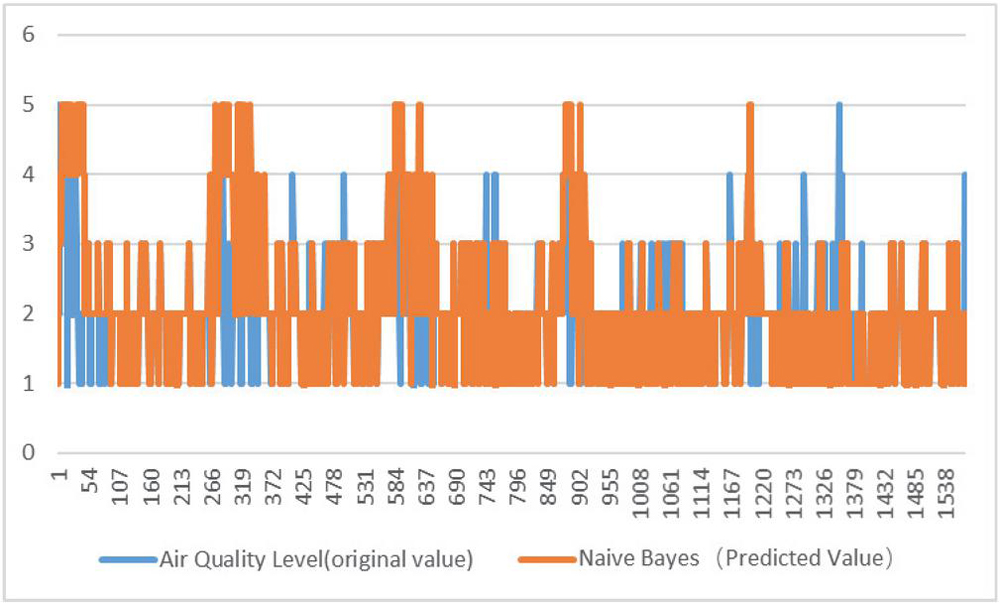
Figure 2 Original and predicted values of training set.

Figure 3 Original and predicted values of prediction set.
The data in Tables 2 and 3 demonstrate that the Naive Bayes Model has the highest accuracy for Chongqing’s air quality assessment and has a good generalization ability,at the same time, through Figures 2 and 3, the effectiveness of naive Bayesian method can be verified again. Through experimental analysis:
(1) When calculating the distance of the sample data, the corresponding weight is given according to the distance, which improves the evaluation accuracy of algorithms such as SVM, XGBoost, bagging, and random forest, but the improvement is limited, and the sample data set distribution of urban air quality is unbalanced, the number of samples with “moderate pollution” and “extremely severe pollution” is relatively small, so the accuracy of evaluation of algorithm models such as SVM, XGBoost, bagging, and random forest is still lower than that of the Naive Bayes Model.
(2) This thesis mainly solves the problem of urban environmental air quality evaluation. Since the air pollutants that cause the decline of urban air quality are not independent for each other, the increase of sulfur dioxide and nitrogen oxides will inevitably affect the rise of PM 2.5. As each feature variable is not independent for each other, it will affect the accuracy of Bayesian model evaluation to some certain extent, but considering that it has fewer data requirements and can handle large sample data with noise and uneven distribution, it can be effectively evaluated the city’s ambient air quality.
5 Conclusion
Evaluation of urban environmental air quality claims exceeding crucially by an increasing number of individuals. There is no doubt that it is particularly important for the construction of ecological civilization. Nowadays, society is developing rapidly. The past evaluation methods are difficult to apply to the era of information and intelligence. Machine learning comes into being with artificial intelligence, mainly based on massive data, with intelligent processing as the core.
This thesis firstly uses wavelet analysis to sort out the original data, and then applies the Naive Bayes algorithm in machine learning to the evaluation of urban environmental air quality to propose a new method of urban air quality evaluation. In order to improve the science and rationality of the evaluation method, through the establishment of the Naive Bayes Model to find the intrinsic mapping relationship between various pollutants in the urban air and the air quality level, and then select Chongqing for experimental verification. The results show that the accuracy of the air quality assessment of Chongqing by the Naive Bayes Model is above 95% on average. This verifies the feasibility of the Naive Bayes Model to evaluate the urban ambient air quality. Finally, by comparing with the SVM, XGBoost, bagging and random forest models in machine learning, it is found that the Naive Bayes Model has the highest accuracy and is much higher than other algorithms. In general, the Naive Bayes Model can accurately and effectively evaluate the urban ambient air quality.
Acknowledgements
Thanks for The National Social Science Fund of China (No. 19BJY077, No. 18BJY093 and No. 17CJY031), the National Natural Science Fund of China (No. 71901044), the Chongqing Normal University Fund (No. 13XWB008), Chongqing Social Science Planning Project (No. 2019WT12, No. 2018PY74), Science and Technology Project of Chongqing Education Commission (No. KJQN201800513 and No. KJQN2019 00537). This paper is grateful to the reviewers for helpful comments.
References
[1] G. Onkal-Engin, I. Demir, H. Hiz, Assessment of urban air quality in Istanbul using fuzzy synthetic evaluation, Atmospheric Environment, 38, No. 23, 3809–3815 (2004).
[2] S. C. Chan, C. T. Lee, Evaluation of the temporal variations of air quality in Taipei City, Taiwan, from 1994 to 2003, Journal of Environmental Management, 86, No. 4, 627–635 (2008).
[3] H. R. Zhang, X. L. Yin, Study on the assessment of atmospheric environment quality in Qingdao from 2004 to 2013 based on AHP, Environmental Science and Management, 40, 7, 180–184 (2015).
[4] Z. Y. Li, The method of composite index of environmental quality, Environmental Science in China, 6, 75–77 (1997).
[5] G. Q. Zhang, Evaluation of ambient air quality in Golmud City by matter element analysis, Qinghai Environment, 2, 78–80 (1997).
[6] Y. Liu, J. Nie, X. Li, X, S. H. Ahmed, W. Y. Lim C. Miao. Federated Learning in the Sky: Aerial-Ground Air Quality Sensing Framework with UAV Swarms. IEEE Internet of Things Journal, 1–1 (2020).
[7] A. Ahilan, et al. Segmentation by Fractional Order Darwinian Particle Swarm Optimization Based Multilevel Thresholding and Improved Lossless Prediction Based Compression Algorithm for Medical Images. IEEE Access, 7, 89570–89580 (2019).
[8] Y. M. Li, Econometric analysis of influencing factors of air quality in Beijing, Theoretical Discussion, 5, 260–261 (2011).
[9] H. J. Wu, X. H. He, Prediction of air quality index based on GA-BP neural network, Journal of Anhui Normal University (Natural Science Edition), 42, 4, 360–365 (2019).
[10] L. Liu, Application of circulation neural network model based on TensorFlow in air quality prediction of Shanghai, Shanghai: Shanghai Normal University (2019).
[11] Basheer, Shakila. Network Support Data Analysis for Fault Identification Using Machine Learning. International Journal of Software Innovation, 7, 2, 41–49 (2019).
[12] M. Mohiddin, V. S. S. Kumar, A low cost air quality monitoring sensor system with arduino uno micro controller board on smart phone and laptop, Advances in Industrial Engineering and Management, 7, 2, 22–29 (2018).
[13] Y. Wang, Application of data mining algorithm based on decision tree in air quality assessment, Nanchang: Nanchang University (2009).
[14] F. Chen, Study of air quality index regression prediction model based on cart algorithm, Journal of Shangrao Normal University, 36, 6, 16–21 (2016).
[15] H. Khelifi, S. Luo, B. Nour, A. Sellami, H. Moungla, S. H. Ahmed, M. Guizani. Bringing Deep Learning at the Edge of Information-Centric Internet of Things. IEEE Communications Letters, 23, 1, 52-55(2019).
[16] F. Guo, L. Y. Xie, Prediction of air quality index based on meteorological factors and improved support vector machine, Environmental Engineering, 35, 10, 151–155 (2017).
[17] S. Q. Hu, Q. W. Jiang, B. Ling, W. D. Yin, Early warning model of air quality monitoring based on support vector machine, Journal of Jiangsu University (Natural Science Edition), 37, 4, 491–496 (2016).
[18] D. W. Zhang, Q. Zhao, Y. F. Xu, Air quality prediction based on long and short term memory neural network model, Journal of Hebei University of Science and Technology, 1, 67–75 (2020).
[19] B. K. Kilinc, The effects of industry increase and urbanization on air pollutants in turkey: A nonlinear air quality model, Applied Ecology and Environmental Research, 17, 4, 9889–9903 (2019).
[20] D. B. Percival, A. T. Walden, Wavelet Methods for Time Series Analysis, Cambridge University Press (2000).
[21] K. S. Kumar, M. Anbarasi, G. S. Shanmugam, A. Shankar, Efficient Predictive Model for Utilization of Computing Resources using Machine Learning Techniques. 2020 10th International Conference on Cloud Computing, Data Science & Engineering (Confluence).
[22] D. J. Hand and R. J. Till, A simple generalization of the area under the ROC Curve for multiple class classification problems, Machine Learning, 45, 2, 171–186 (2001).
[23] M. Anbarasan, B. Muthu, C. Sivaparthipan, R. Sundarasekar, S. Kadry, S. Krishnamoorthy, A. A. Dasel. Detection of flood disaster system based on IoT, big data and convolutional deep neural network. Computer Communications, 150, 150–157 (2020).
[24] Q. Jia, Urban air quality assessment method based on GIS technology, Applied Ecology and Environmental Research, 17, 4, 9367–9375 (2019).
[25] J. Gao, H. Wang, and H. Shen. Task Failure Prediction in Cloud Data Centers Using Deep Learning. IEEE Transactions on Services Computing, 1–1 (2020).
Biographies

Jun Duan received a master’s degree in economics from Southwest University in 2007 and a doctor’s degree in management from Chongqing University in 2019. He has been teaching in the School of Economics and Management of Chongqing Normal University since July 2007. His current research interests include energy economy and big data mining and analysis.

Qi Ren received a bachelor’s degree in engineering from Zhengzhou University in 2002 and a master’s degree in agriculture from Chongqing Normal University in 2018. Since July 2012, he has been teaching at Chongqing Urban Management Vocational College, and his current research interests include machine learning and data analysis.
Strategic Planning for Energy and the Environment, Vol. 42_1, 119–136.
doi: 10.13052/spee1048-5236.4217
© 2022 River Publishers