A Quantile Regression Analysis of the Impact of Electricity Production Sources on CO $_{2}$ Emission in South Asian Countries

Shapan Chandra Majumder¹, Liton Chandra Voumik^2,*, Md. Hasanur Rahman³, Md. Maznur Rahman² and Mohammad Nasir Hossain¹

¹Department of Economics, Comilla University, Cumilla-3506, Bangladesh
²Department of Economics, Noakhali Science and Technology University, Noakhali, Bangladesh-3814
³Department of Economics, Sheikh Fazilatunnesa Mujib University, Jamalpur-2000, Bangladesh
E-mail: scmajumder_71@yahoo.com; litonvoumik@gmail.com; hasanur.cou@gmail.com; egreen@yahoo.com; nasir_das@yahoo.com
*Corresponding Author

Received 26 June 2022; Accepted 30 August 2022; Publication 31 January 2023

Abstract

This study wants to fill a gap in the empirical literature by looking at how the sources of electricity affect CO $_{2}$ emissions in South Asian countries. Because of the consistent production levels and economic growth in South Asian countries, energy generation is becoming a key issue. The data, which covers from 1972 to 2015, is subjected to quantile regression (QR). The quantile regression coefficients’ findings are statistically significant at a 1% level of significance. According to the regression results, all energy generation sources and associated variables have a positive impact on CO $_{2}$ emissions. Coal-fired power plants have a bigger impact on the environment than other types of pollution. On the other hand, renewable energy sources have the minimum impact on environmental degradation. Possible alternatives for reducing carbon dioxide emissions instead of coal, oil, and gas-based energy production sources have been presented. The policy implications also suggest that environmental policy should be improved by applying renewable energy, wind energy, hydroelectric sources, and nuclear energy. The link between economic growth and energy concentration needs to be looked into more with the help of more economic indicators and the parameters of electricity-generating sources.

Keywords: Climate change, CO $_{2}$ emissions, Electricity production sources, Energy consumption, Quantile Regression.

1 Introduction

Carbon dioxide (CO $_{2}$ ) and other toxic gas emissions have been a major concern in environmental, health, and development studies over the last century, owing to its multiple detrimental impacts. CO $_{2}$ is one of the key greenhouse gases (GHGs) and one of the prime causes of global warming, greenhouse effects, and climate change (Rahman et al. 2020; Murshed 2020). Researchers, academics, policymakers, and a variety of other groups from all over the world are currently focused on it. CO $_{2}$ emissions are a direct result of rapid industrialization, artificial development, environmental degradation, and an ever-increasing population. Since the industrial revolution, CO $_{2}$ absorption has surpassed pre-industrial levels by 2.5 times, according to WMO’s yearly greenhouse gas report (WMO 2019).

The focus of this research was to determine the influence of different sources of power on CO $_{2}$ emissions. This study’s quantitative information comes from the World Bank’s World Development Indicators (WDI). Every low-income, developing, and developed country in the world aims for economic growth and rapid development. In the South Asian context, this concept is particularly important because all countries in this region are either undeveloped or developing countries in the economic context. This South Asian region is home to more than 40% of people who live below the poverty line (Daily Times 2014). India, Bangladesh, Sri Lanka, Pakistan, and the Maldives are trying to combat this poverty, unemployment, malnutrition, and underdevelopment quickly by investing in electricity because it is one of the key indicators of rapid development. The per-head GDP of this area is $1,779, which is still much lower than that of the lower and middle-income countries in the world, which is $4,497 and $10,636 respectively (World Bank, 2019). So, these countries’ GDP growth shows that the scenario will be changed within 10 years in the future.

According to World Bank (2021), Nepal experienced the 4th position in GDP growth rate among the South Asian countries and the annual GDP growth rate in 2021 was 4.25%. Bangladesh has been secured the second position with a growth rate 6.94%. India was experiencing a 8.95% growth rate and ranked 1st. Similarly, Pakistan ranked 3rd in the South Asian area with a 5.97% growth rate and Sri Lanka currently has the lowest GDP growth rate in the region, at 3.66%. On the other hand, it is thrilling that South Asian countries are growing and increasing well in recent years, at the same time environmental degradation has increased (Usman et al. 2021). However, You et al. (2022) state that, the middle income group and lower income group of countries has positive cause to raise CO $_{2}$ emission but higher income group has no significant contribution. Factors such as population increase, energy production, infrastructural advancement as well as financial sector growth can have a significant impact on the economic growth or development of a country. Population growth, energy production and usage, and trade openness, according to the following studies and other researches such as Ardakani et al. (2018) Aslani et al. (2019), Rahman and Majumder, (2022), all result in increased emissions of greenhouse gases like CO $_{2}$ . All of these factors have contributed to economic prosperity, but they have also had a severe impact on the environment. Because the methods used by researchers are unplanned, they come up with these problematic results. There are omitted variables biases, varied sample sizes in studies, and a wide range of countries’ characteristics and peculiarities (Ozturk 2010; Zeshan and Ahmed 2013).

South Asia is one of the most populous regions in the world. When it comes to population density, some countries rank higher than others. According to the UN (2015) report, Bangladesh has the highest population density in this region, and the world position was 12th. India is also a vastly populated country, also home to the world’s second-largest populated country in the world. Others South Asian countries like Nepal, Pakistan, Sri-Lanka Maldives and others population growth is raising (Mishra and Dash, 2022). Populations are considered essential for economic growth, but they are not the only factor. As a result of the enormous population, there is a wide range of goods and services to choose from. On the other hand, overpopulation causes excess consumption and overuse of energy, which leads to CO $_{2}$ emissions. In addition, past studies have only examined the influence of financial development and renewable energy on CO $_{2}$ emissions by utilizing either panel or time-series data, which is a limitation. Few studies such as Poudel (2020), Sebos et al. (2020), Bozkurt (2021) Guo and Zhao (2022), Batool et al. (2022) and others have examined the impact of renewable energy production and consumption on CO $_{2}$ emissions at the sub-component level, according to our knowledge. Our empirical analysis reveals that the impact of electricity production sources on CO $_{2}$ emissions is unclear. While it is widely proved that power production has a negative connection with carbon emissions, electricity production from different sources increases carbon emissions and economic growth.

In 2012, The Guardian (2012) published that India’s economy was ranked as the 4th largest economy in the world, and in terms of total CO $_{2}$ emissions from energy consumption, it was ranked 3rd in the world. On the other hand, when considering carbon emissions, India’s neighbouring countries like Pakistan, Bangladesh, Sri Lanka, and Nepal ranked 33rd, 57th, 90th, and 137th. In 2018, India produced CO $_{2}$ equivalent to 1.80 metric tons, Bangladesh produced 0.51, Pakistan and Sri-Lanka produced 0.98 and 1.00 metric tons, respectively (World Bank, 2021). Furthermore, CO $_{2}$ emissions (metric tons per capita) in South Asia were 1.5, 6.1 in the European Union, 6.5 in East Asia and the Pacific, and 5.6 in the Middle East and North Africa (World Bank, 2021). However, the dynamic causality between electricity production, CO $_{2}$ and economic growth has been analysed by Bento and Moutinho (2016), where the authors explore that electricity production from renewable sources has a large contribution to emission reduction. The reduction policies should be based on modern technology as well as using renewable sources of electricity production where non-renewable sources emit more carbon into the atmosphere (Xiaosan, 2021). Atekin’s (2022) paper aims to evaluate countries according to the energy-environment-sustainability triangle using ARAT, CRITIC, and CODAS-Sort. The results reveal that developed countries are in a better situation than developing and underdeveloped countries in terms of sustainable energy and environmental concerns. Therefore, as the literature reviews support that electricity production and CO $_{2}$ emissions are interconnected, the inclusion of CO $_{2}$ is very crucial in our model. Moreover, from academic and research perspectives, we saw only a few types of research done on this topic and the quantile regression methodologies by using panel data in South Asia that address this issue.

2 Literature Review

However, the enormous consumption of different energy sources and their impacts on CO $_{2}$ emissions are becoming a great threat to the present and future generations. Perimeter droughts, ice melting, rising sea levels, global warming, and heatwaves are already being considered everywhere in the world. These negative impacts on the environment create a hazardous situation. Urry (2015) added that there is an increase in CO $_{2}$ and other greenhouse gases in the atmosphere that are responsible for these calamities. They also collected data on increasing temperatures on land and at sea. In a study of eleven Asian countries, Rahman (2017) found that the absorption of greenhouse gases rose by 34% between 1990 and 2013, with over 80% of this increase due to CO $_{2}$ emissions. This is in accordance with Amri’s (2017) claim that CO $_{2}$ emissions have risen from 67 million metric tons to 134 million metric tons. Hence, Meltzer (2016) concluded that different types of environmental pollution are responsible for more than 150,000 deaths per year. Ozturk (2010) confirmed there were relationship between electricity consumption from different sources and economic expansion; additionally, other energy consumption and growth. Measurement of climate change mitigation initiatives can be used for a wide range of purposes, including guiding policy design, boosting the implementation of policies, measuring the effectiveness of policies, justifying budget allocation, and attracting climate financing (Sebos et al. 2021).

According to Tabli (2017) and Wang (2017) a number of factors, including population size, renewable energy, fossil fuel energy consumption, the carbon intensity of energy, emphasis on economic growth, nuclear energy, overcrowded urbanization, harmful air pollutants, such as PM10, PM2.5, SO $_{2}$ , NO $_{2}$ , CO, benzopyrene (one of the pentacyclic hydrocarbons), and overpopulation, have been identified as causing the rise in global CO $_{2}$ emissions. One of the environmental impacts that have been considered for geothermal plants is the release of CO $_{2}$ into the environment because it needs a high temperature (300 $^{\circ}$ F to 700 $^{\circ}$ F). Despite the fact that the magnitudes of impacts from fossil fuel power plants are greater (Armannsson 2003). Due to the production and consumption of various geothermal energies in the environment, it has been seen that the concentration of chemicals is available in the environment. Also, ecological, biological, and chemical changes happen in the environment (Rehman et al. 2022). Begum et al. (2015) found an inverse relationship between economic growth and carbon dioxide emissions for Malaysia, Mohsin et al. (2022) also found an inverse relationship between economic growth and carbon dioxide emissions in the long run for Europe and Central Asia. This paper suggests energy innovation; i.e. green energy usage or low-carbon innovations mitigate environmental degradation problems and exhilarate sustainable economic growth. Rahman and Velayutham (2020) and Rahman et al. (2021) have investigated whether there is a causal relationship between energy consumption and industrialization. Whatever the energy, economic growth, and CO $_{2}$ emissions in South Asia investigated by Siddique et al. (2020) and Zafar et al. (2020). Many researchers, like Charfeddine and Kahia (2019), Nathaniel et al. (2020), have looked into the relationship between renewable energy, production, and CO $_{2}$ emissions in the Middle East and North African region. Their empirical analysis revealed that there is a negative association between the standard shock and the use of renewable energy as well as the response in terms of carbon dioxide emissions to that shock. Even after attaining a highly developed economy, electrification has taken place in all areas of the industrial and service sectors in South Korea, one of the Asian tigers, resulting in a continual expansion of the concentration of energy resources. Also contributing to increased electrification in manufacturing sectors were the development and expansion of the information and communication technology (ICT) industries as well as cheap electricity rates. They also discovered that there is a positive association between electrification and harmful gas emissions (Cho 2007; Yoo 2005).

In China, energy consumption in main industries, such as manufacturing, raw materials, mining, and chemicals, has also flourished since 1990. Also, it dramatically increased electrification in all industries and households within three decades (Wang et al. 2007). As a result, numerous studies have previously been published that analyzed CO $_{2}$ emissions from the consumption of energy sectors in both developing and wealthy countries. Their research deconstructed the driving forces of CO $_{2}$ emissions caused by the energy generation sectors, and they also presented country-by-country comparisons, allowing for the identification of each country’s consumption, emissions, and policy.

Table 1 Brief summary of relevant literature

Author	Data	Methodology	Findings
Mehmood (2021)	1996Q1–2019Q4; Panel Data; South Asia	ARDL Model	Volatile growth pattern and environmental degradation showed in Bangladesh, Pakistan, India and Sri-Lanka by considering energy utilization in long run.
Ali et al. (2017)	1980–2013; Panel Data; South Asia	Co-integration and EKC	Nonrenewable energy has tremendous impact on raising environmental pollution.
Khan et al. (2022)	1972–2017; Panel Data; South Asia	Co-integration, FMOLS and EKC	Individual country like Bangladesh has marvelous impact on raising environmental pollution by considering non renewable energy.
Khan et al. (2018)	1981 to 2015; Time Series; Pakistan	VECM, CCR and FMOLS	Electricity production from coal source raises the emission on the other hand renewable energy reduces the emission level.
Source: Authors Compilation.

According to a review of previous literature, case studies that examined CO $_{2}$ emissions in the electricity generation sector and examined the influence of various factors were mainly composed of a few countries, and the countries of interest were primarily developing countries in Southeast Asia and the Middle East, such as China, Saudi Arabia, Vietnam, and others, as well as developed countries in Europe, according to a review of previous literature. Because Chen (2018) and Szymczyk et al. (2021) analyzed emissions of CO $_{2}$ at the level of the country rather than the sector level, and rather than using data from individual countries, they primarily relied on aggregate panel data from 35 OECD countries, it is difficult to draw direct comparisons with the findings of this study.

3 Methodology

3.1 Data and Variables of the Study

During the period from 1972 to 2015, annual panel data was obtained from the World Development Indicators (WDI), a World Bank database that contained information on the development of South Asian countries. Here is a list of the variables that we used in our analysis. This study considered countries such as India, Pakistan, Sri-Lanka, Bangladesh, and Nepal, where the rest of the countries were not used in this study because of several limitations. Those limitations are: lack of data availability, data inconsistency, missing year observations, and others. That’s why this study considered those countries which have available and consistent data.

Table 2 Introduction of selected variables

Name of the Variables	Variables in Log Form	Elaboration of the Variables	Sources
CO $_{2}$	L(CO $_{2}$ )	CO $_{2}$ emissions (kt)	WDI
Coal	L(Coal)	Electricity produced by coal (% of total)	WDI
Gas	L(Gas)	Electricity produced by natural gas (% of total)	WDI
Oil	L(Oil)	Electricity produced by oil (% of total)	WDI
Renewable	L(Renew)	Electricity produced by renewable sources, excluding hydroelectric (% of total)	WDI
Source: WDI (2020).

3.2 Econometric Model Specification

To investigate the impact of electricity production from different sources on CO $_{2}$ emissions, our independent variables are electricity produced by coal, oil, natural gas, and renewable sources (excluding hydroelectric sources) on CO $_{2}$ , and we have followed the famous methodological approach.

The effect between dependent and independent variables can be precisely by the Equation (1) below:

C O_{2} = f (Coal, Gas, Oil, Renew)

(1)

Now, the multivariable econometric model is that:

C O_{2}_{i, t} = β_{0} + β_{1} {Coal}_{i, t} + β_{2} {Gas}_{i, t} + β_{3} {Oil}_{i, t} + β_{4} {Renew}_{i, t} + ε_{i, t}

(2)

The log transformation has been taken in Equation (3.2).

$L n C O_{2}_{i, t}$	$= β_{0} + β_{1} {LCoal}_{i, t} + β_{2} {LGas}_{i, t}$
	$+ β_{3} {LOil}_{i, t} + β_{4} {LRenew}_{i, t} + ε_{i, t}$	(3)

Where,

$β_{0}$ is the intercept term,

$β_{1}, β_{2}, β_{3}$ , and $β_{4}$ are the slope coefficient. The $ε$ is present the residual, and $i$ presents the cross section country, $t$ present the time.

3.3 Quantile Regression (QR Regression)

Buchinsky (1994) points out that, In order to describe the feasible heterogeneous impacts, we identify the qth-quantile (0 $<$ q $<$ 1) of the dependent variable as impermanent distribution, given a set of $X_{i}$ variables, as follows:

Q_{q} (\frac{y_{t}}{x_{t}}) = a_{q} + x_{t} \cdot β_{q} + u_{t} \cdot α_{q}

(4)

Where $y_{t}$ the CO $_{2}$ emission through time is, $u_{t}$ signify for unobservable factors. A vector of independent variables ( $X_{i t}$ ) is also included. Cameron and Trivedi (2010) demonstrate that Equation (4) inference based on the qthquantile regression requires the minimization of the residual’s absolute value using the subsequent objective function:

$Q (β_{q})$	$= m i n_{β} \sum_{i = 1}^{n} ∥ y_{t} - x_{t} β_{q} ∥$
	$= m i n [\sum_{y_{t} = x_{i} β} q \| y_{t} - x_{i t} β_{q} \| + \sum_{y_{t} < x_{i t} β} (1 - q) \| y_{t} - x_{i t} β_{q} \|]$	(5)

Following Canay (2011), the assessment approach is divided into two phases. In the first stage, the restrictive mean of u $_{t}$ is determined and analyzed. During the following stage, this component is subtracted from the original dependent variable, and after that, the typical quantile regression assessment is performed.

4 Empirical Result

4.1 Principal Components Analysis and Descriptive Statistics

To analyze and understand relationships in continuous multivariate data, principal component analysis (PCA) is one of the important tools. When the dataset is large and the researcher needs to reduce it dimensionally, the PCA techniques are very helpful in this case. At the same time, it’s trying to minimize information loss by converting a large set of variables into a smaller one. Whatever, the result of descriptive statistics is shown in Table 3. Although there are a few variables in this paper, we do not need PCA to remove them. We applied PCA because we wanted to ensure that the variables were independent of one another whether or not. At this point, the researcher has to decide how to move forward. Providentially, Eigen values and screen plots are two important statistical and linear algebra calculations that help us make the decision. PCA does not apply to binary data. Binary data shows meaningless results. When there are a substantial number of correlated variables, a multivariate analysis problem can be struck out. In this case, PCA can play a great role in reducing dimensions.

Overall, PCA (Table 4) aims at reducing unnecessary variables and making a large set of variables into a small set. All variables don’t need to contribute to all PCA. Some variables contribute to PCA1, some are PCA2, and some are PCAn. The PCA1 is strongly correlated with three of the dependent and independent variables. The PCA1 expands as $L (C O_{2})$ , $L (C o a l)$ , and L(Renew) are increased. They all seem to be affected by each other. When one does better, the rest of the group tends to do better as well. It is possible to see this component as a way of evaluating the quality of coal, gas, and renewable energy sources (excluding hydroelectric). Furthermore, it is seen that the PCA1 correlates most strongly with the L(Renew). On the basis of the correlation coefficient of 0.594, we may conclude that this principal component is predominantly a measure of the L(Renew). When four variables indicate a rising trend, the second main component grows as a result. On the other hand, L(Coal) is negatively correlated with PCA2. L(Oil) is highly correlated with PCA2. Also, PCA2 can be viewed as an evaluation of how electricity production from oil sources is related to PCA2. The PCA3 shows an increase in L(Coal) related to L(Oil). This proposed that places with a high log of coal would also be likely to have a better log of oil. $L (C O_{2}$ ) is positively correlated, but the value is very small. On the other hand, PCA4 demonstrates that three variables are positively correlated and two variables are oppositely correlated. L(Coal) is highly correlated with PCA4 and L(Renew) is negatively correlated and the magnitude is very high. Similarly, at last, the PCA5 is positively correlated with four of the independent variables and negatively correlated with the only dependent variable.

It is seen that the PCA5 increases with increasing $L (C o a l)$ , L(Gas), L(Oil), and L(Renew). It shows a strong correlation with L(Coal) and L(Gas), but a very minute relationship with L(Oil) and L(Renew). On the other hand, a highly negative correlation is visible with $L (C O_{2}$ ). When it comes to coal, natural gas, and renewable energy, this component can be thought of as a measure of the quality of the electricity produced by these sources (excluding hydroelectric). Furthermore, it is seen that the PCA5 negatively correlates most strongly with the $L (C O_{2}$ ).

Table 3 Synopsis of descriptive statistics

	L(CO $_{2}$ )	L(Coal)	L(Gas)	L(Oil)	L(Renew)
Mean	13.56	3.64	2.12	1.53	$-$ 1.38
Median	13.75	4.21	2.28	1.48	$-$ 0.81
Maximum	14.62	4.31	4.42	3.65	1.64
Minimum	11.15	$-$ 2.00	0.39	0.57	$-$ 6.93
Std. Dev.	0.87	1.67	0.89	0.70	2.56
Skewness	$-$ 1.43	$-$ 2.68	0.54	1.69	$-$ 0.79
Kurtosis	4.66	8.71	4.10	6.05	2.55
Source: Author’s Calculation.

Table 4 Principal component analysis (PCA)

Variables	PC 1	PC 2	PC 3	PC 4	PC 5
L(CO $_{2}$ )	0.587	0.290	0.049	0.276	$-$ 0.702
L(Coal)	0.535	$-$ 0.316	0.363	0.458	0.523
L(Gas)	0.076	0.701	$-$ 0.485	0.285	0.432
L(Oil)	$-$ 0.102	0.570	0.773	$-$ 0.231	0.114
L(Renew)	0.594	0.005	$-$ 0.181	$-$ 0.761	0.187
Source: Author’s Calculation.

When PCA1 and PCA2 explain a major portion of the variance in the data, the data can be visualized by projecting the observations onto the span of the first two principal components. In a PCA, this projection of the data is known as a “score plot.” Also, there is another projection called the “loadings plot,” where the variable vectors on the span of the PCs are projected.

A bi-plot is a famous exploratory graph that overlays score plot and a loading plot in a particular graph. The bi-plot points illustrate the projected observations and the vectors show the projected variables. For selected data, PCA1 and PCA2 explain 73% of the variance in the five-dimensional data. Therefore, with a two-dimensional set of principal components, these data are decorated and well-approximated. For convenience, the scatter plot, or score plot, and the vector plot, or loadings plot, are shown below for the iris data. Notice that there is a different scale between the loading plot and the score plot.

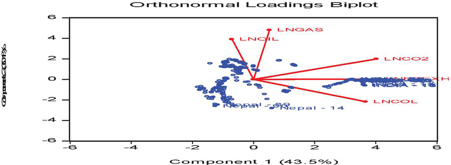
Figure 1 Orthonormal loadings biplot.

Source: Author’s Calculation.

4.2 Results of the Panel Unit Root Test

The panel unit root test is extremely important and crucial in panel data analysis because it allows you to distinguish between stationary and non-stationary properties of the dependent and independent variables. It is also used to identify the presence of a stationary or non-stationary relationship between the dependent and independent variables.

Table 5 Unit root test results

Variables
Panel Unit
Root Test	L(CO $_{2}$ )	L(Coal)	L(Gas)	L(Oil)	L(Renew)
At Level
Im, Pesaran and Shin W-statistics	2.434	0.193	2.017	$-$ 1.719	0.944
ADF – Fisher Chi-square	9.603	9.492	1.793	20.107	0.344
Levin, Lin & Chut	2.581	$-$ 0.450	1.117	$-$ 1.011	0.787
At 1st Difference
Im, Pesaran and Shin W-statistics	$-$ 6.398***	$-$ 7.451***	$-$ 7.578***	$-$ 9.989***	$-$ 5.655***
ADF – Fisher Chi-square	56.314***	61.811***	57.071***	97.063***	24.384***
Levin, Lin & Chu t	$-$ 5.498***	$-$ 7.329***	$-$ 3.672***	$-$ 6.293***	$-$ 6.719***
Note: 1%, 5%, 10% significance level denoted by *, and * respectively. Presume as trend and intercept.
Source: Author’s Calculation.

A variety of panel unit root tests are available in the existing literature, each with its own set of characteristics. At the raw data and first difference levels, the results of the unit root test for dependent and independent variables are shown in Table 5. As shown in this example, whereas H0 is regarded as non-stationary and has a unit root, H1 is considered stationary and has no unit root, whereas H0 is not considered stationary and does not have any unit root. At I(1), the L(CO $_{2}$ ), L(Coal), L(Gas), and L(Renew) variables are stationary, as shown in the table. When data is altered from one period to the preceding period, however, all are stationarily at the first difference level. It was decided to use a 5% significance threshold for both levels and the first difference, and the results show that the null hypothesis is rejected at the first difference in all variables. As a result, all variables in first differenced data are classified as stationary variables, and there is no unit root. At I(1), all series are stationary variables, and now it is easy to predict the data. All p values less than 0.01 mean all are significant with a 1% significance level because it is less than alpha ( $=$ 0.01).

Overall, we expect that dependent and independent variables will follow a unit root procedure. Researchers’ specific significance levels are often 0.1 (10%) or 0.05 (5%), so when the p-value is less than or equal to a specified significance level, the null should be rejected. At 1%, the first difference level is called the “high significance level.” Even at the first difference level, our approximate p-value is less than 0.01, so we would reject the null in all these cases.

4.3 Quantile Regression QR (Regression)

Finally, the paper employs the quantile regression (QR) approach to examine the comprehensive relationship between CO $_{2}$ emissions and electricity generation sources in South Asian countries.

Table 6 Quantile regression

Variable	Coefficient	Std. Error	t-Statistic	Prob.
L(CO $_{2}$ )
L(Coal)	0.443***	0.061	7.266	0.000
L(Gas)	0.427***	0.047	9.106	0.000
L(Oil)	0.248***	0.056	4.404	0.000
L(Renew)	0.126***	0.011	11.841	0.000
C	8.035***	0.165	48.651	0.000
R-squ.	0.470
Adj R-squ.	0.460
Quasi-LR statistic	333.863***
Note: 1%, 5%, 10% significance level designated by *, and * orderly.
Source: Author’s Calculation.

According to the findings presented in Table 6, between 1972 and 2015, all of the independent factors had a positive impact that was statistically significant on the change in CO $_{2}$ emissions in the South Asian countries. Thus, a 1% increase in electricity production from coal sources results in a 0.44 percent increase in CO $_{2}$ emissions, whereas a 1% increase in electricity production from gas sources results in a 0.427% increase in environmental degradation. A similar condition to environmental degradation is made by renewable and oil-based electricity generation. CO $_{2}$ emissions increase by 0.126 % when the amount of electricity generated from renewable sources increases by 1%. The environmental impact of renewable energy production is the lowest of all the options. Because of this, renewable electricity generation has the potential to reduce CO $_{2}$ emissions more than other options. The development of renewable energy sources to produce electricity is commonly assumed to be beneficial in environmental science, climate change study, and policy analysis (von Weizsäcker et al. 2014; Fischer-Kowalski, 2011). At the beginning of 2010, 83 countries and all 50 states in the United States had policies in place to encourage the production of electricity from renewable energy sources. This included solar, wind, geothermal, and hydroelectric power. Typically, these policies were defined to exclude large-scale hydroelectric facilities (REN21 2010, National Research Council 2010). On the ground, it appears that the production of renewable energy could potentially replace the production of fossil fuels, and this would allow a reduction in CO $_{2}$ emissions despite an increase in economic production. Using renewable energy to generate electricity in South Asia is expected to have a lower environmental impact than conventional methods, according to the study. Hydro, solar, wind, and geothermal power are all examples of renewable energy sources.

Quantile regressions have been performed on data and the results are shown in Table 7 of this study. L(Coal) coefficients are positive up to the 50th quantile in the regression estimates and negative in the upper quantiles, rising in value from the lower quantiles to the middle quantiles and decreasing in higher quantiles, but statistically significant from the first to fourth quantile up. Up to the 50th quantile of the distribution, we find negative coefficients on L(Oil) and L(Renew) variables. On the other hand, from the 50th to the last quantile, the coefficients of L(Oil) and L(Renew) variables are positive. Although only L(Gas) statistically insignificant up to 50th quantiles, L(Oil) becomes statistically insignificant beyond the 50th quantile. The null hypothesis is rejected because p-value is less than 1%. Hence it is concluding that, the data is not symmetrical. On the other hand, in the Figure 2, L(Coal) rose in response to rising quantiles, as seen by process estimates. L(Oil) and constant increase in proportion to the quantile. When quantiles rise, L(Gas) fluctuates as well. In order to derive the quantile process estimates with fixed effects, tau 0.9 reveals the detrimental influence. There are findings of diagnostic test for the panel quantile regression in Table 8 where the assumption that the residuals are regularly distributed is called normality.

Table 7 Quantile slope equality test

Test Summary	Chi-Sq. Statistic	Chi-Sq. d.f.	Prob.
Wald Test	36.89***	8	0.00
Restriction Detail: b(tau_h) – b(tau_k) = 0
Quantiles	Variable	Restr. Value	Std. Error	Prob.
0.25, 0.5	L(Coal)	0.391***	0.118323	0.0009
	L(Gas)	0.024396	0.065201	0.7083
	L(Oil)	$-$ 0.313***	0.096321	0.0011
	L(Renew)	$-$ 0.048**	0.020676	0.0194
0.5, 0.75	L(Coal)	$-$ 0.148**	0.077715	0.0553
	L(Gas)	$-$ 0.295***	0.099587	0.003
	L(Oil)	0.039	0.051347	0.4401
	L(Renew)	0.054***	0.017243	0.0015
Note: 1%, 5%, 10% significance level designated by *, and * orderly.
Source: Author’s Calculation.

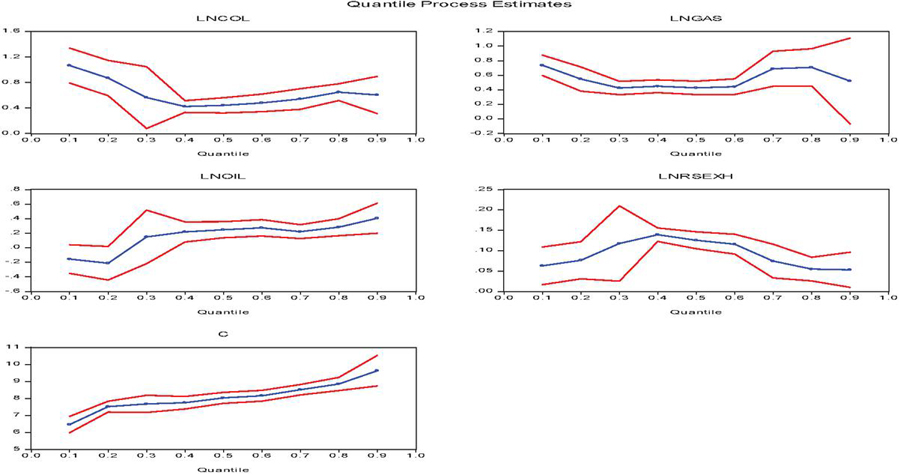
Figure 2 Quantile process estimates.

Source: Author’s Calculation.

Table 8 Residual diagnostics test

Model	Normality Test
	J-B Stat	Prob
QREG	0.56	0.75
Source: Author’s Calculation.

5 Conclusion

This study’s goal has been to examine the impact of power generating methods on CO $_{2}$ emissions in South Asian nations, i.e., L(Coal), L(Gas), L(Oil), and L(Renew) using yearly data spanning between 1972 and 2015. The quantile regression methodology was applied to get an empirical investigation, which presents the advantage of analysing the effects of electricity production sources on CO $_{2}$ emissions. This method lets us provide a more detailed explanation of the overall dependence of electricity production from different sources on CO $_{2}$ emissions, compared to several methods that were applied to such types of research, such as Ordinary Least Square (OLS), Generalised Least Square (GLS), or ARDL. It has been observed that the effect of all independent variables is positive and highly significant. However, the slopes of different quantiles are volatile in the quantiles slope equality test. The magnitudes of electricity production from coal and gas sources have higher coefficients. Also, the relationship between electricity production from renewable sources and environmental degradation is positive, but the magnitude is lower. So, electricity production from renewable sources is preferable to other sources. Overall, a perceptible positive relationship was found between electricity production sources and CO $_{2}$ emissions in South Asian countries. Research suggests that renewable energy consumption-related policy implementation has not yet achieved the desired level, and so electricity production in these nations is still heavily reliant on non-sustainable energy sources. Attributed to huge electricity production, industrialization, economic growth, and an expanding population, the global increase in CO $_{2}$ emission levels has been largely due to human activities and behaviors. An enormous threat to human health and the environment is posed by this. Numerous variables were found to be statistically significant when quantile regression was used to analyze the data. In other words, the majority of the variables examined had a direct impact on the amount of CO $_{2}$ emitted throughout the experiment.

6 Policy Implication and Future Research

On the basis of the findings, the following policy implications can be made. In order to assure effective and sensible power usage sustain long-term economic growth in the investigated regions, strategies for electricity, business, banking sector development, and economic expansion might be simultaneously established. Second, given the financial and energy growth has a detrimental impact on the atmosphere (bad effects on Pollutant emissions), in theory, these nations can cut their electricity consumption and aspirations for growth; nonetheless, this is not the preferred course of action. Investigating integrated systems is the greatest option for these nations. Using clean, renewable energy sources will help cut down on CO $_{2}$ emissions even further. Thirdly, despite a decrease in using coal and oil, have an adverse influence on these countries economic growth because coal and oil are also determined to be injurious to the environment. As a result, in order to create tradable commodities, a rise in the usage of eco-friendly and environment-safe technology a sensible choice. Fourth, substantial budget implies that CO $_{2}$ emissions are also on the rise. The pressing necessity is to create sustainable financial systems while taking into account methods. Last but not least, studies on carbon pricing through taxes, a trade system, or a cap. The advancement of technology for renewable power can also be beneficial in cutting down emissions of carbon dioxide.

References

Amri F (2017) Intercourse across economic growth, trade, and renewable energy consumption in developing and developed countries. Renewable and Sustainable Energy Reviews, 69:527–534.

Ali S, Anwar S, Nasreen S (2017) Renewable and Non-Renewable Energy and its Impact on Environmental Quality in South Asian Countries. Forman Journal of Economic Studies, 13.

Armannsson H (2003) CO $_{2}$ emission from geothermal plants. In: Proceedings Of International Geothermal Conference (pp. 56–62). Geothermal Association of Iceland, Rey-kjavik, Iceland.

Armannsson H Kristmannsdottir H (1992) Geothermal environmental impact. Geothermics, 22: 869–880.

Aytekin A (2022) Energy, Environment, and Sustainability: A Multi-criteria Evaluation of Countries. Strategic planning for energy and the environment, 41(3), 281–316.

Ardakani SR, Hossein SM, Aslani A (2018) Statistical approaches to forecasting domestic energy consumption and assessing determinants: The case of Nordic countries. Strategic Planning for Energy and the Environment, 38(1), 26–71.

Aslani A, Ghiasi MM, Safari M (2019) Analysis of the Robustness of Canada Economy and Energy Supply/Demand Fluctuations. Strategic Planning for Energy and the Environment, 38(3), 7–26.

Begum RA, Sohag K, Abdullah SMS, Jaafar M (2015) CO $_{2}$ emissions, energy consumption, economic and population growth in Malaysia. Renewable and Sustainable Energy Reviews 41: 594–601.

Bozkurt E (2021) Renewable Energy and Economic Efficiency in the Framework of Sustainable Development: Malmquist Index and Tobit Model. Strategic Planning for Energy and the Environment, 163–174.

Batool Z, Raza SMF, AliS, Abidin SZU (2022) ICT, renewable energy, financial development, and CO $_{2}$ emissions in developing countries of East and South Asia. Environmental Science and Pollution Research, 29(23), 35025–35035.

Bento JPC, Moutinho V (2016) CO $_{2}$ emissions, non-renewable and renewable electricity production, economic growth, and international trade in Italy. Renewable and sustainable energy reviews, 55, 142–155.

Buchinsky M (1994) Changes in the US wage structure 1963-1987: Application of quantile regression. Econometrica: Journal of the Econometric Society, 62: 405–458.

Cameron AC Trivedi PK (2010) Microeconometrics using stata (Vol. 2). College Station, TX: Stata press.

Canay IA (2011) A simple approach to quantile regression for panel data. The Econometrics Journal, 14: 368–386.

Charfeddine L, Kahia M (2019). Impact of renewable energy consumption and financial development on CO $_{2}$ emissions and economic growth in the MENA region: A panel vector autoregressive (PVAR) analysis. Renewable Energy 139: 198–213.

Chen J, Wang P, Cui L., Huang S et al (2018) Decomposition and decoupling analysis of CO $_{2}$ emissions in OECD. Applied Energy, 231: 937–950.

Cho Y, Lee J, Kim TY (2007) The impact of ICT investment and energy price on industrial electricity demand: Dynamic growth model approach. Energy Policy, 35: 4730–4738.

Daily Times (2014). 40% Poor Live in South Asia, Staff Report. March 06.

Fischer-Kowalski, Marina, ed. 2011. Decoupling Natural ResourceUse and Environmental Impacts from Economic Growth. NewYork, NY: UNEP Publishing.

Guo Y, Zhao M (2022) Research on Sustainable Energy Development From the Perspective of Focusing on Carbon Peaking and Neutrality. Strategic Planning for Energy and the Environment, 345–362.

Khan MB, Saleem H, Shabbir MS, Huobao X (2022) The effects of globalization, energy consumption and economic growth on carbon dioxide emissions in South Asian countries. Energy & Environment, 33(1), 107–134.

Khan MT., Ali Q, Ashfaq M (2018) The nexus between greenhouse gas emission, electricity production, renewable energy and agriculture in Pakistan. Renewable Energy, 118, 437–451.

Meltzer JP (2016). Financing low carbon, climate resilient infrastructure: the role of climate finance and green financial systems. Climate Resilient Infrastructure: The Role of Climate Finance and Green Financial Systems (September 21: 2016).

Mehmood U (2021) Renewable-nonrenewable energy: institutional quality and environment nexus in South Asian countries. Environmental Science and Pollution Research, 28(21), 26529–26536.

Murshed M (2020). An empirical analysis of the non-linear impacts of ICT-trade openness on renewable energy transition, energy efficiency, clean cooking fuel access and environmental sustainability in South Asia. Environmental Science and Pollution Research 27: 36254–36281.

Mishra AK, Dash AK (2022) Connecting the Carbon Ecological Footprint, Economic Globalization, Population Density, Financial Sector Development, and Economic Growth of Five South Asian Countries. Energy Research Letters, 3(2), 32627.

Mohsin M, Naseem S, Sarfraz M, Azam T (2022) Assessing the effects of fuel energy consumption, foreign direct investment and GDP on CO $_{2}$ emission: New data science evidence from Europe & Central Asia. Fuel, 314, 123098.

Nathaniel S, Anyanwu O, Shah M (2020) Renewable energy, urbanization, and ecological footprint in the Middle East and North Africa region. Environmental Science and Pollution Research, 27(13), 14601–14613.

Ozturk I (2010) A literature survey on energy-growth nexus. Energy Policy, 38: 340–349.

Rahman MH, Majumder SC, Debbarman S (2020) Examine the Role of Agriculture to Mitigate the CO $_{2}$ Emission in Bangladesh. Asian Journal of Agriculture and Rural Development, 10: 392–405.

Poudel DD (2020) Asta-Ja Framework: A Peaceful Approach to Food, Water, Climate, and Environmental Security Coupled with Sustainable Economic Development and Social Inclusion in Nepal. Strategic Planning for Energy and the Environment, 243–318.

Rahman MM (2017) Do population density, economic growth, energy use and exports adversely affect environmental quality in Asian populous countries?. Renewable and Sustainable Energy Reviews, 77:506–514.

Rahman MH, Majumder, SC (2022) Empirical analysis of the feasible solution to mitigate the CO $_{2}$ emission: evidence from Next-11 countries. Environmental Science and Pollution Research, 1–19.

Rahman MM, Velayutham E (2020) Renewable and non-renewable energy consumption-economic growth nexus: new evidence from South Asia. Renewable Energy 147: 399–408.

Rahman MH, Ruma A, Hossain MN et al (2021). Examine the Empirical Relationship between Energy Consumption and Industrialization in Bangladesh: Granger Causality Analysis. International Journal of Energy Economics and Policy, 11: 121–129.

Rehman A, Ma H, Ozturk I, Ulucak R (2022) Sustainable development and pollution: the effects of CO $_{2}$ emission on population growth, food production, economic development, and energy consumption in Pakistan. Environmental Science and Pollution Research, 29(12), 17319–17330.

Sebos I, Progiou AG, Kallinikos L (2020) Methodological framework for the quantification of GHG emission reductions from climate change mitigation actions. Strategic Planning for Energy and the Environment, 219–242.

Siddique HMA, Majeed DMT, Ahmad DHK (2020) The impact of urbanization and energy consumption on CO $_{2}$ emissions in South Asia. South Asian Studies, 31: 745–757.

Szymczyk K, Şahin D, Bağcı H, Kaygın CY (2021) The effect of energy usage, economic growth, and financial development on CO $_{2}$ emission management: an analysis of OECD countries with a High environmental performance index. Energies, 14: 4671.

Talbi B (2017) CO $_{2}$ emissions reduction in road transport sector in Tunisia. Renewable and Sustainable Energy Reviews, 69:232–238.

The Guardian (2012) World Carbon Emissions: the League Table of Every Country. 21 June, 2012.

UN (2015) List of Countries by Population Density. United Nations Department of Economics and Social Affairs, Statistics Times retrieved from. http://statisticstimes.com/population/countries-by-population-density.phpon20.

Urry J (2015) Climate change and society. In Why the Social Sciences Matter. Palgrave Macmillan: London, UK, pp. 45–59.

Usman M, Anwar S, Yaseen MR et al (2021) Unveiling the dynamic relationship between agriculture value addition, energy utilization, tourism and environmental degradation in South Asia. Journal of Public Affairs, e2712.

von Weizsäcker EU (2014) Decoupling: Technological Opportunities and Policy Options: Executive Summary. In Ernst Ulrich von Weizsäcker (pp. 219–238). Springer, Cham.

Wang A, Lin B (2017) Assessing CO $_{2}$ emissions in China’s commercial sector: Determinants and reduction strategies. Journal of Cleaner Production, 164:1542–1552.

Wang W, Mu H, Kang X, et al. (2010) Changes in industrial electricity consumption in china from1998 to 2007 Energy Policy, 38: 3684–3690.

WMO (2020) Greenhouse Gas Bulletin (GHG Bulletin) - No.16: The State of GreenhouseGases in the Atmosphere Based on Global Observations through 2019. World Meteorological Organization (WMO). Published by: WMO; 2020.

World Bank (2021). World development indicators. Accessed at: http://www.worldbank.org/data/ online data bases.

Xiaosan Z, Qingquan J, Iqbal KS, Manzoor A, Ur RZ (2021) Achieving sustainability and energy efficiency goals: assessing the impact of hydroelectric and renewable electricity generation on carbon dioxide emission in China. Energy Policy, 155, 112332.

Yoo SH (2005) Electricity consumption and economic growth: Evidence from Korea. Energy Policy 33: 1627–1632.

You, W, Zhang Y, Lee, CC (2022) The dynamic impact of economic growth and economic complexity on CO $_{2}$ emissions: An advanced panel data estimation. Economic Analysis and Policy, 73, 112–128.

Zafar A, Ullah S, Majeed MT, Yasmeen R (2020) Environmental pollution in Asian economies: Does the industrialisation matter? OPEC Energy Review, 44:227–248.

Zeshan M, Ahmed V (2013) Energy, environment and growth nexus in South Asia. Environment, development and sustainability, 15:1465–1475.

Biographies

Shapan Chandra Majumder is an Associate Professor at the Department of Economics, Comilla University, Bangladesh. Dr. Majumder has completed his PhD. from the School of Economics, University of Shandong, P. R. China. He has teaching experiences around 13 years. He has taught at different Bangladeshi universities and has published many articles in SCOPUS (Q1, Q2, Q3, Q4), SSCI, SCI-E and ESCI Indexed journals. Dr. Majumder has eleven years of university teaching experience. His areas of interest cover foreign direct investment inflows in developing countries, one belt one road, infrastructure development, environmental economics, energy economics, development economics, international trade and applied econometrics.

Liton Chandra Voumik is an assistant professor at the department of economics at Noakhali Science and Technology University, Bangladesh. The fields of environmental economics, development economics, and labor economics are the primary topics of Liton’s Research. Liton earned a master’s degree from Middle Tennessee State University in the United States. He earned a bachelor’s degree in economics from the University of Chittagong.

Md. Hasanur Rahman is a full-time faculty member and Lecturer at the Department of Economics, Sheikh Fazilatunnesa Mujib University (SFMU), Jamalpur-2000, Bangladesh. Mr. Rahman has completed his Bachelor of Social Science (BSS) and Master of Social Science (MSS) in Economics from Comilla University (CoU), Cumilla-3506, Bangladesh. He has published many articles in SCOPUS (Q1, Q2, Q3, Q4), SSCI, SCI-E, and ESCI Indexed journals. His areas of interest are development economics, international trade, environmental economics, energy economics and econometrics.

Md. Maznur Rahman is a full-time faculty member at the Department of Economics, from the Noakhali Science and Technology University, Bangladesh. He is current PhD student at Mizoram University, India. He has published several articles in indexed journals. His areas of interest are in trade, development economics, FDI, and health economics.

Mohammad Nasir Hossain is a full-time faculty member at the Department of Economics, from the Comilla University, Bangladesh. He has published several articles in ISI and Thomson Reuters indexed journals. His areas of interest are in environmental economics, microfinance, development economics, international trade, health economics and urban economics.

Strategic Planning for Energy and the Environment, Vol. 42_2, 307–330.
doi: 10.13052/spee1048-5236.4223
© 2023 River Publishers