LSTM Based Forecasting of PV Power for a Second Order Lever Principle Single Axis Solar Tracker
Krishna Kumba*, Sishaj P. Simon, Kinattingal Sundareswaran and Panugothu Srinivasan Rao Nayak
Department of Electrical and Electronics Engineering, National Institute of Technology, Tiruchirappalli, Tamil Nadu, India
E-mail: kumba.krishna@gmail.com
*Corresponding Author
Received 31 January 2022; Accepted 08 November 2022; Publication 31 January 2023
Abstract
Nowadays solar power generation has significantly improved all over the world. Therefore, the power estimation of photovoltaic (PV) using weather parameters presents the future management of energy utilization in power system planning. This article presents the power forecast of the Second Order Lever Principle Single Axis Solar Tracker (SOLPSAST) system. A deep neural network is developed using Long Short Term Memory (LSTM) and is validated on sunny, cloudy and partially cloudy days. The performance of the proposed LSTM in comparison with Support Vector Machine (SVM) has improved the Mean Absolute Proportion Error (MAPE) forecasts accuracy to 4.29%, 5.16%, and 4.82% for sunny, cloudy and partially cloudy days, respectively. Also, the estimated Mean Relative Error (MRE) value of the LSTM model for sunny, cloudy and partially cloudy days is 3.19%, 4.10%, and 4.02%, respectively. Finally, the forecasted power generation of the SOLPSAST system’s monthly average and annual generation is found to be 2.45 Wh, and 29.44 kWh, respectively.
Keywords: LSTM method, photovoltaic, PV forecasting, single axis solar tracker, solar energy.
1 Introduction
Sun is a significant supplier of solar energy to the Earth. Solar power emerges as a viable alternative energy source that can meet a larger portion of the world’s expanding energy demands. Therefore, photovoltaics (PV) has an important role in increasing the worldwide energy demand scenario. PV systems convert solar radiation into electricity and play a critical part in our power system’s energy transition. The generation and performance of the PV system depend on several factors such as uncertainties of weather (solar irradiance, module temperature, outside temperature, cloud cover, wind speed, and humidity of the atmosphere), timing, and operating condition. Consequently, this poses complications in power system grid supervision with the PV systems. In supervision, the cost of operations and maintenance currently has an important impact on the profit of solar PV systems. Technical development offers the opportunity to generate clean energy at a low cost.
Solar power must be estimated in the short and long term by the energy market. An accurate PV generate forecast is required for the safe and worthwhile integration of PV in smart grids [1, 2]. PV power estimation in PV power plants is an extremely dynamic research field. Moreover, forecasting PV power generation ensures the power grid’s safety and supports reducing the operational expenses of these solar energy sources. PV power forecasting is primarily done in three categories. They are physical, numerical, and machine learning models [3]. A physical model is based mostly on the interplay of physics rules based on radiation and weather [4]. Numerical weather forecasting [5], sky imager [6], and satellite perception [7] are the three subtypes of physical models. Fuzzy system [8], Grey system [9], Markov chain [10], Autoregressive [11], and Regression method [12] are the five sub-models of statistical models [13]. The above methods strongly rely on historical data to be able to predict future time series [14].
Support vector machine [15], and artificial neural networks (ANN) are sub-models of the machine learning model. Support vector machine (SVM) models are significant kernel-based learning models that can provide accurate predictions using kernel tricks. The SVM is a reliable approach for predicting solar PV power. The main applications of SVM algorithms are non-linear regression problems like PV power forecasting. Choosing appropriate kernel functions and accelerating training speed throughout its quadratic programming process are challenging tasks in SVM algorithms [16]. Hence, researchers have merged SVM methods with other predictive approaches to provide more accurate short-term PV forecasting estimates.
A subset of artificial intelligence is machine learning (AI). This improves the accuracy of software programmers in anticipating outcomes without requiring them to be particularly developed. It can extract extensively complicated nonlinear characteristics efficiently and have the capability of mapping straight from input to output. The decision tree [17], The most extensively utilized algorithm for forecasting time series data is the ANN model [18, 19]. Machine learning algorithms have significantly increased the predicting precision of PV power that can use historical information. The approaches for predicting PV generation using ANN and Long Short-Term Memory (LSTM) are listed below.
Adel Mellit et al. have forecasted the 24 hr ahead power of PV using solar radiation and ambient air temperature data and achieving an RMSE value of 32.98–75.48% with the ANN method [20]. A. Yona et al. has forecasted day ahead PV power using weather data consisting of solar radiation, relative humidity, wind speed, and temperature. The RMSE value attained was 0.478–1.176 of ANN methods [21]. F. Almonacid et al. has forecasted one hour ahead of PV power using solar radiation, cell temperature, and IV curve of the PV module data. The RMSE value realized is 3.38% with this method [22]. Changsong Chen et al. designed an online PV power predicting model that uses weather data such as solar radiation, humidity, wind speed, and ambient temperature to forecast PV power 24 hours ahead of time. MAPE value for the ANN method is 9.33–10.80% [23]. Ercan Izgi et al. has forecasted 0–60 mins PV power using past values of 750 W solar PV panel data. The RMSE value obtained is 19.95–54.11 [24]. Hugo T.C et al. forecasted one and two hours ahead of PV power using the production of past data. The RMSE value realized is 107 kW and 160.79 kW of the ANN method [25]. Jie Shi et al. has forecasted one day ahead of PV power utilizing numerical weather predictions from weather parameters such as cloudy day, clear sky, rainy day, and foggy. The RMSE average value attained is 2.10 [26]. Monowar Hossain et al. forecasted one day and one hour ahead of PV power using average solar irradiation, module temperature, wind speed, and air temperature. The RMSE value achieved is 35.78 [27]. Jun Liuet al. has forecasted 24 hours ahead of the PV power using solar irradiance, wind speed, humidity, and ambient temperature. The MAPE value obtained is 6.38–8.27 [28]. The above literature review [20–28] shows that the ANN forecasts PV power using weather data. However, the arithmetic metrics parameters RMSE and MAPE are not close to true values. Furthermore, the difference between the forecasted and actual power of the ANN method is slightly greater. The literature review of forecasted PV power using LSTM networks is as follows.
A. Gensler et al. has forecasted day ahead PV power using weather predictions from the diffuse and direct solar, clear-sky filter, and temperature parameters. They achieved an RMSE value of 0.0713 using Auto LSTM methods [29]. Woonghee Lee et al. forecasted day ahead PV power using weather data received from a rough guess of the national weather center solar irradiation, temperature, humidity, wind speed, and precipitation. The RMSE value obtained is 0.0987–0.2520 using LSTM and Convolutional Neural Networks (CNN) methods [30]. Donghun Lee and Kwanho Kim forecasted one hour ahead of PV power using real-world weather dataset solar radiation, temperature, humidity, and cloudiness month of the. The RMSE value achieved is 0.563–0.874 using the LSTM method [31]. Abdel-Nasser and Mahmoud forecasted one hour ahead of PV power using datasets from many locations over for a year. The RMSE value ranges between 82.15–136.87 for five different LSTM methods [32]. Yoonhwa Jung et al. forecasted monthly PV power using a weather dataset of solar irradiation, wind speed, humidity, temperature, precipitation, duration of sunshine, and cloud cover. The RMSE value realized is 7.416% [33]. Mingming Gao et al. forecasted day ahead and one-hour PV power using condition mean values of solar radiation, highest and lowest temperature, and relative humidity. They recorded a RMSE value 4.62–17.3% and 5.34–13.86% [34, 35]. Fei Mei et al. forecasted the day ahead power of PV using historical PV power, solar radiation, and temperature. The RMSE value obtained is 58.9834–71.1089 using LSTM Quantile Regression Averaging [36]. Kejun Wanget al. forecasted PV power using temperature, phase average active power, global and solar diffuse horizontal radiation, and wind velocity. The RMSE value acquired is 0.621 [37]. Fei Wang et al. forecasted day-ahead PV power using normal solar radiation and temperature and achieved an RMSE value of 6.29–8.83% [38]. Biaowei Chen et al. forecasted five minutes ahead of PV power using historical PV data, global and diffuse horizontal solar radiation, temperature, and humidity. The average enhancement of RMSE by this method is 30.01% [39].
In recent decades, machine learning techniques such as ANN, SVM, and LSTM are the developed as models to forecast PV power in the above literature. According to the aforementioned literature review, deep learning networks are good at forecasting PV power using renewable meteorological conditions. However, these techniques use past data from the PV forecasting models, and various factors also affect the output of PV. The majority of forecasting techniques do not analyse the relationship between the various factors and PV output. The deep learning network mostly outperforms the conventional ANN and SVM networks in predictions. The majority of the investigations are carried out for fixed systems using meteorological factors for one hour and day-ahead output power forecast. However, no work is projecting the output power of a PV tracking system based on weather conditions. Moreover, the energy estimation of the PV system throughout the year is not been done so far. Therefore, this work evaluates the forecasting of single-axis solar tracker [40] PV power using a deep neural network. The following is a summary of this paper’s significant contributions:
i. An LSTM-based network is developed to forecast the SOLPSAST system power for the day ahead and throughout the year.
ii. The performance of the LSTM model in forecasting is evaluated for different weather conditions (sunny, cloudy, and partially cloudy days).
iii. The developed LSTM model is compared with two well-known PV power forecasting techniques (SVM and Backpropagation Neural Network (BPNN)) to show its efficiency.
The rest of the article is structured as follows. Performance evaluation of the LSTM model is discussed in Section 2. Methodology and used data set are discussed in Section 3. Section 4 gives the arithmetic evaluation measures. Section 5 describes the SOLPSAST system’s operational capabilities. Section 6 contains the SOLPSAST generated and LSTM, SVM and BPNN models forecasted results and discussion. The conclusions are presented in Sections 7.
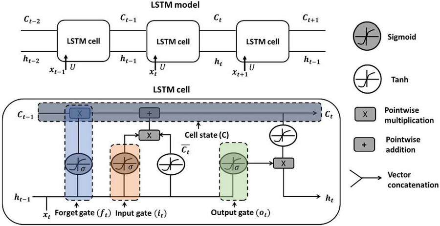
Figure 1 LSTM model and LSTM cell structure.
2 Long Short Term Memory (LSTM) Formation and Simulation Tool
The LSTM as opposed to traditional feedforward neural networks uses feedback connections. The LSTM formation and LSTM cell structure are shown in Figure 1. The LSTM cell has four basic components: (i) cell (C), (ii) forget gate (f), (iii) input gate (i), and (iv) output gate (o). Wherein, x and h are the input layer and hidden layer. The cell state values and three genes govern the movement of data in and out of the cell at random time intervals [41]. The variables’ calculation formulas are as follows:
Where W, U are weight for , , . is the activation function.
Here, the significant aim is to develop a proper learning rate for an LSTM forecast model. MATLAB deep learning toolbox is used in this work and using this toolbox the LSTM model is developed. The stochastic gradient descent technique and Adam algorithms are recommended by MATLAB as the optimization approach for LSTM implementation [42].
3 Methodology and Dataset
The proposed LSTM for SOLPSAST system for power forecasting is presented in flowchart (ref Figure 2). In this flow chart, the sequence of actions carried out is presented. The meteorological data inputs (solar radiation (G), ambient temperature (), module temperature ()) and the output data sets (SOLPSAST system’s power) are recorded placed at a latitude of 10.78. The meteorological data is gathered from the Davis Pro2 weather station and generated SOLPSAST system output power is taken using a data logger. All these systems are free from shading effects. The weather and generated power data are considered from 6.00 AM to 6.00 PM. All these data are standardized into normalized form with five min intervals. So, the total number of samples for a given day will be 144. For both current and future needs, the database will store all input data.
Data pre-processing is performed to confirm the data set entry form to the LSTM model. Any peak and non-stationary data elements in the input data forecasting model indicate that the PV power forecasting model is improperly trained, resulting in a significant prediction error. Consequently, the data pre-treatment techniques are used for parsimony, missing values, and feature scaling. Without assuming a certain model relationship, machine learning can learn on its own and make accurate predictions. Initial time-series data is divided into training and testing groups. The simulation uses data from 91 days in total. In the simulation, 87 days are used for training, and 4 days are used for testing. The power generated by the SOLPSAST system is the target data set. After being trained using training data, the LSTM network will be put to the test with targeted data.
The PV forecasting model can find the most relevant data to forecast PV outputs after it has the G, , and data of the target day. The forecast model can locate similar seasonal samples and the same weather type. These days should have the closest solar radiation. Therefore, the test day’s PV production curve will likely follow a similar pattern. Here, the historical data of power values already obtained on test days are used to compare the forecast output of LSTM model. The data obtained on testing days are used to determine the error metrics. Equation (1) can be used to compute the temperature of PV module cells. Where NOCT is the normal operating cell temperature [21].
| (1) |
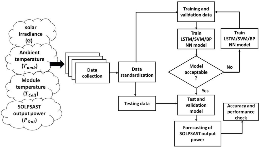
Figure 2 Flowchart of power forecasting method.
4 Performance Evaluation
Four arithmetic metrics are used to assess the LSTM, SVM, and BPNN forecast models of the SOLPSAST system, whose advantages are explained as follows [43–45]:
Mean Absolute Error (MAE) is the number of mistakes within paired observations that demonstrate the same feature.
| (2) |
where n denotes the number of samples.
In Root Mean Square Error (RMSE) the mistakes are squared before being averaged, and it gives significant errors a comparatively high weight.
| (3) |
The Mean Absolute Proportion Error (MAPE) is a related metric that displays errors as a percentage of the actual data. The most significant advantage of MAPE is that it provides a straightforward and natural means of measuring the degree or impact of mistakes.
| (4) |
Mean Relative Error (MRE) is highly useful when comparing measured data in units. It will give how far the forecasted value is from measured values. Here, is the system capacity.
| (5) |
Moreover, the coefficient of discrimination (COD) is usually used for performance regression analysis. The COD can be calculated using Equation (6).
| (6) |
Diebold-Mariano Test
The performance of the forecast models with respect to each of the individual models is statistically analyzed using Diebold-Mariano (DM). In order to go one step further, DM test is used to find whether this difference between two or more forecasts is significant or not, or simply because of the sample’s unique selection of data values [46, 47]. The DM criterion determines if the two forecasts are significantly different based on general assumptions. Let Error1 () and Error2 () are the residuals for the two forecasts.
| (7) |
is loss-differential of time series. The MAE error statistic of function as
| (8) |
for , the autocorrelation function defines as
| (9) |
For , the DM can be obtained using Equation (10).
| (10) |
In the sufficient value of .
Thus, if , where is the two-tailed critical value of the standard normal distribution, there is a considerable discrepancy in the forecasts.
| (11) |
Where is the level of significance which is equal to 5% or 0.05.
5 SOLPSAST System
The SOLPSAST system is operating at a latitude of 10.78. The SOLPSAST system is shown in Figure 3. The second-order lever principle governs the operation of the SOLPSAST system. The PV panel of the SOLPSAST system is designed by balancing the mass of water with the part mass of the PV panel on one side (left) of the fulcrum and the mass of the PV panel on the other side (right) [40]. During sunrise, the PV module of the SOLPSAST system faces west. A DC pump is employed to fill the water tank by drawing water from the collector tank in the ground at 6.00 AM of sunrise. The pump fills the tank with enough water to shift the PV module to face the sun directly to the east.
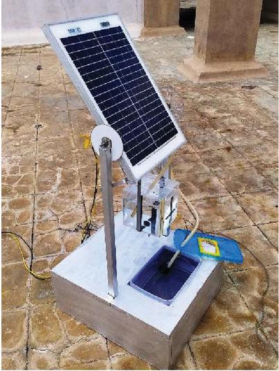
Figure 3 SOLPSAST system.
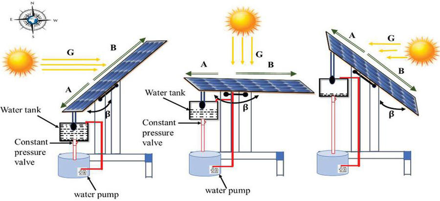
Figure 4 Morning, Afternoon, and Evening variation of SOLPSAST system.
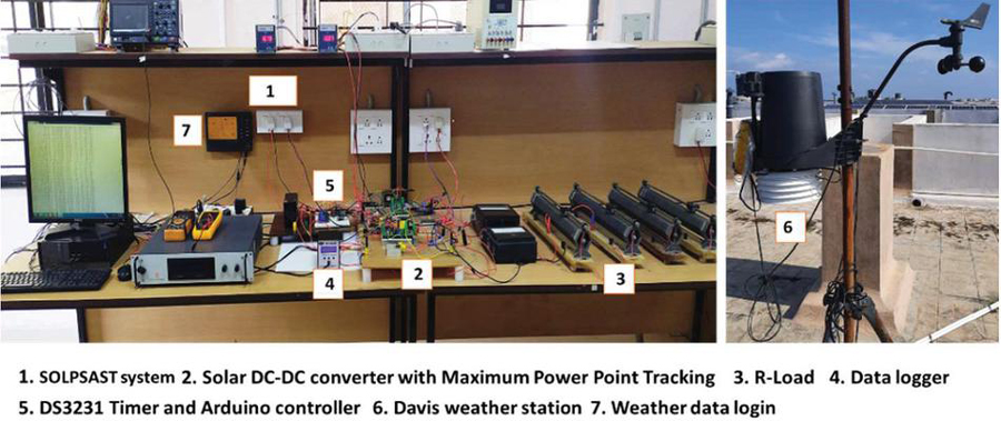
Figure 5 DC-DC converter of SOLPSAST with the data monitoring system, Controller and Weather station.
A switching automation system controls the ON and OFF of the DC water pump. A constant pressure valve is placed at the bottom of the water tank. The desired filled water tank on the PV panel’s left side will commence leaking continuously due to the constant pressure value. When water leaks from the orifice of the water tank, the total weight left side to the fulcrum will reduce while the weight right side to the fulcrum will be the same as before. Hence in order to counterbalance the weight reduction left side to the fulcrum a clockwise torque act upon the SOLPSAST system around the fulcrum axis. So, it will tend to rotate clockwise from morning to evening. The flow of water through the orifice is controlled by a constant pressure valve such that it takes sunrise to sunset time to rotate 45 to 45. Consequently, the PV module continuously tracks the sun from sunrise to sunset. The movements of the SOLPSAST system in three time zones (morning, noon, and evening) are depicted in Figure 4. To harvest maximum power from the SOLPSAST system, the maximum power point tracking (MPPT) approach with the Perturb and Observe (P&O) algorithm is used in this system. Figure 5. exhibits DC to DC converter of the SOLPSAST system, as well as the Davis vantage PRO2 weather station, and data logging system. The automation system which uses an Arduino controller is also shown in the same figure. The technical specifications of the solar panel employed in this work is shown in Table 1.
Table 1 Technical specifications of solar panel
| Number of Cells | NOCT | |||||
| 20 W | 36 | 21.6 V | 17.24 V | 1.31 A | 1.16 A | 47 2 |
6 Results and Discussion
The input data parameters solar irradiance, and ambient temperature are logged in the Davis vantage PRO2 (ref Figure 5) weather station, and module temperature is recorded using a data logger. The plot for the solar irradiation (G) data that is used in the simulation is shown in Figure 6. The test site’s average solar irradiation of the year is about 5.42 kW/m. The ambient temperature (), as well as the SOLPSAST system cell temperature, are shown in Figure 7. The year’s average ambient and cell temperatures are 32.97C and 40.67C, respectively.
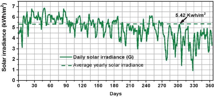
Figure 6 Solar irradiance.
The standardization procedure is required to pre-process the data because the dimensions of each type of data in the data collection are not uniform. Standardization converts all data into the range [0, 1], which aids in the generalization of the LSTM forecast model and reduces the model’s computation time. The standardization formula is given in Equation (12). Where, , , and are original data, input samples maximum and minimum values respectively.
| (12) |
The forecasting model’s output is still normalized; to compare with actual values, the output must be denormalized. For denormalization, Equation (13) is used.
| (13) |
Where , is after normalization data. , and are normalized forecasting and forecasting values.
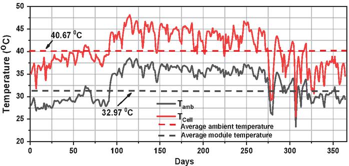
Figure 7 Ambient and module cell temperatures.
In this study, the LSTM model of the SOLPSAST system consists of several learning variables. Multiple trials are conducted and determined the best number of hidden layers and hidden neurons required for the forecast model to produce the most accurate results. The number of LSTM model layers (L) is varied from 1 to b and the layers for which MAPE minimum are fixed. Once the layers are fixed, change the number of neurons (N) for all layers (L) from 1 to c and fix the number of neurons for which MAPE minimum. Equation (14) is used to select the best LSTM design for the three inputs and one output.
| (14) |
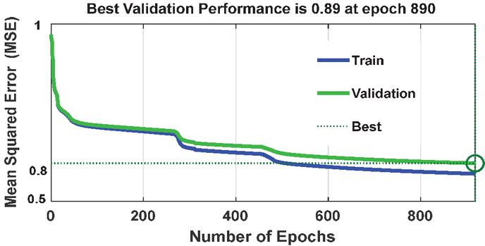
Figure 8 Training and validation of LSTM model.
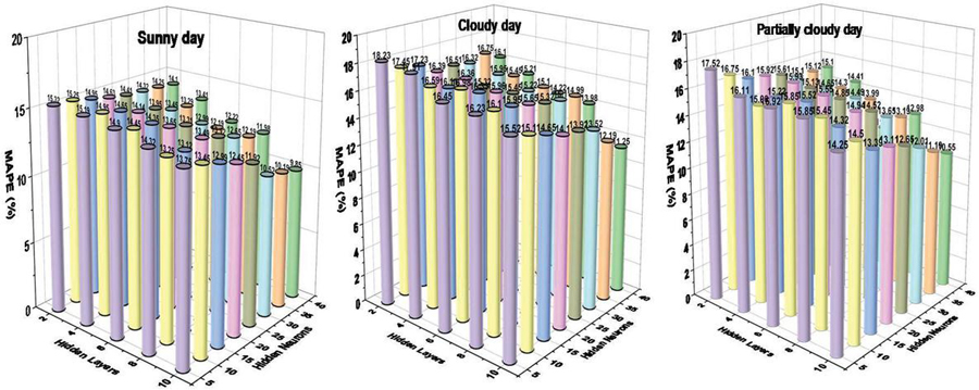
Figure 9 Optimal selection of LSTM model.
Figure 8 depicts the LSTM forecasting model’s training and validation. The training data set is used to train the LSTM model, the verification set is used to fine-tune the LSTM model’s parameters, and the test set is utilized to evaluate the model’s forecasting performance. The MAPE (%) of the trained LSTM forecast model is shown in Figure 9 for three different weather conditions (sunny, cloudy, and partially cloudy). The maximum MAPE (%) values on sunny, cloudy, and partially cloudy days with 2 hidden layers and 5 hidden neurons are 15.32, 18.23, and 17.52, respectively. The minimum MAPE (%) values on sunny, cloudy, and partially cloudy days with 10 hidden layers and 40 hidden neurons are 9.85, 11.25, and 10.55, respectively. So, majorly the LSTM model produces better accuracy with 10 hidden layers and 40 hidden neurons.
Moreover, this paper compares the LSTM performance with six SVM models using the following kernels: Linear SVM (), Quadratic SVM (), Cubic SVM (), Fine Gaussian SVM (), Medium Gaussian SVM (), and Coarse Gaussian SVM (). For regression applications, several approaches use nonlinear kernel functions. The , radial basis function (RBF) [27] is one of the efficient kernel functions. The kernel function of the nonlinear radial basis is given in Equation (15).
| (15) |
Where and are the input space vector and the feature vector generated from the training or the test samples, and (0.58): variance.
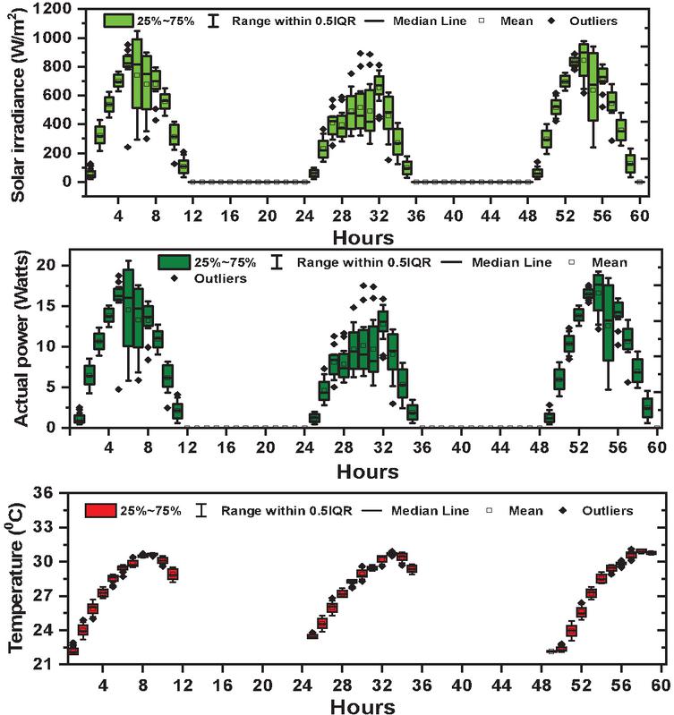
Figure 10 Box plot of solar radiation, ambient temperature, and actual power.
In addition, we compare the LSTM performance with BPNN also. The feed-forward BPNN is the most widely used artificial neural network architecture. The training process of a network is based on the optimization of weights in all nodes’ connection and bias terms. This process is repeated until the forecasted output layer values are as close to the actual outputs as possible. The functions defined in the BPNN model has 3-inputs, 10-hidden layers, 40-hidden neurons, and 1-output. The Sigma activation function and the Levenberg Marquart rule are employed. The total number of iterations is 1500.
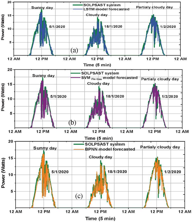
Figure 11 Actual and forecasted power of (a) LSTM, (b) SVM, and (c) BPNN models.
Figure 10 depicts a box plot of the SOLPSAST system’s solar radiation, ambient temperature, and actual power on sunny, cloudy, and partially cloudy days. On three different days, the average sun irradiation of the testing site is 451.54 W/m, 394.40 W/m, and 493.50 W/m. The average ambient temperature (T), as well as the SOLPSAST system average cell temperature for the 3 days are (28.88C, 27.81C, 31.13C) and (35.88C, 31.13C, 38.88C), respectively. The actual power and forecasted power of LSTM, , and BPNN models for 3 days are shown in Figure 11. Here, the figures show the forecasted output power signal that appears to respond to each swing and track its movement, mirroring the overall behavior of the measured output data. Figure 12 shows the forecasted data is very near to the observed test data. Hence, the LSTM, , and the BPNN model is fit for power forecasting. The actual generated power of on sunny, cloudy, and partially cloudy days is 104.78 Wh, 80.19 Wh, and 90.14 Wh, respectively. However, the forecast power is estimated as (101.54 Wh, 77.08 Wh, 86.59 Wh) using LSTM, (95.24 Wh, 69.44 Wh, 70.84 Wh) using and (93.44 Wh, 69.44 Wh, 79.75 Wh) using BPNN.
The linear regression investigation between measured and estimated power is evaluated. Figure 13 shows the scatter plot of the generated and forecast power of the LSTM, , and BPNN models during sunny, cloudy, and partially cloudy days. The SOLPSAST coefficient of discrimination R value for the 3 days is 0.9759, 0.9612, and 0.9734. The R value of the SOLPSAST’s LSTM model is good in contrast to the , and BPNN models. Moreover, the statistical performance evaluation of the LSTM, SVM and BPNN models for the SOLPSAST system is given in Table 2. Furthermore, the MRE (%) of LSTM, SVM, and BPNN models are presented in Table 3.
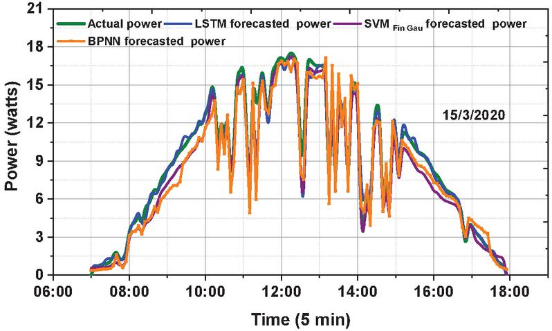
Figure 12 Actual and forecasted power of LSTM, SVM, and BPNN models.
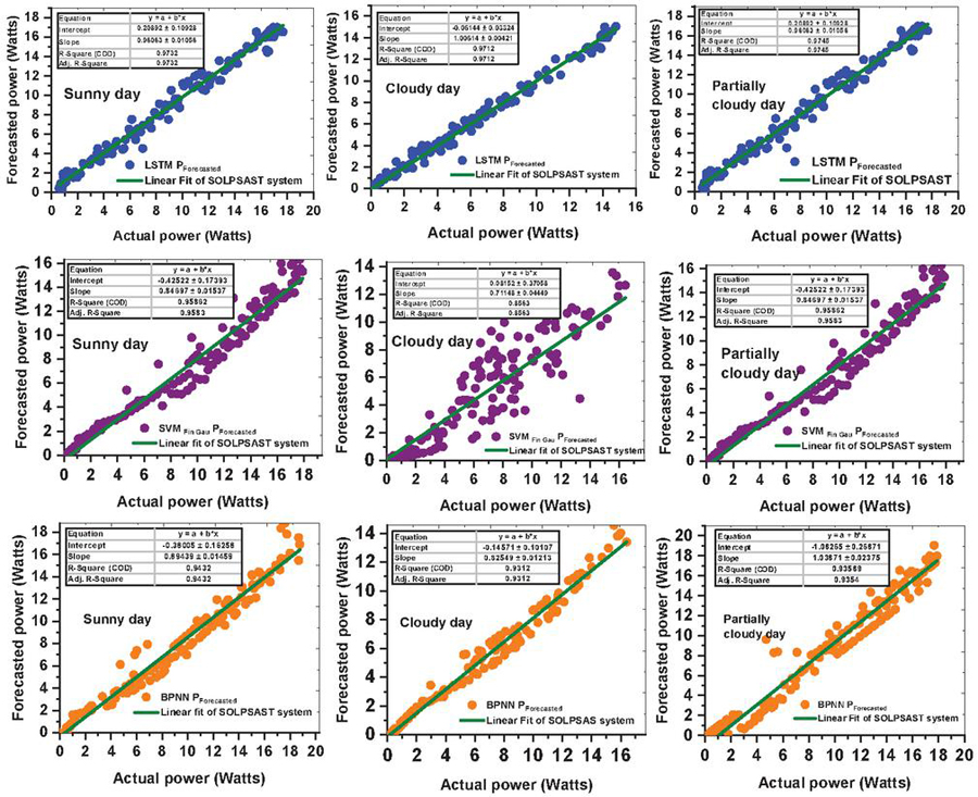
Figure 13 Linear fit curve of actual and forecasted power LSTM, SVM, and BPNN models.
Table 2 Statistical performance of LSTM, SVM, and BPNN models
| Sunny Day | Cloudy Day | Partially Cloudy Day | |||||||
| Model | MAE | RMSE | R | MAE | RMSE | R | MAE | RMSE | R |
| LSTM | 0.35 | 5.08 | 0.97 | 0.50 | 5.71 | 0.96 | 0.49 | 5.55 | 0.97 |
| 1.87 | 7.38 | 0.81 | 1.49 | 7.12 | 0.83 | 1.52 | 7.31 | 0.81 | |
| 2.10 | 8.12 | 0.89 | 1.47 | 7.13 | 0.84 | 1.57 | 7.33 | 0.86 | |
| 1.49 | 7.13 | 0.84 | 1.48 | 7.14 | 0.82 | 1.62 | 7.45 | 0.86 | |
| 1.46 | 7.10 | 0.95 | 1.44 | 7.09 | 0.85 | 1.26 | 6.95 | 0.95 | |
| 1.49 | 7.12 | 0.79 | 1.59 | 7.34 | 0.79 | 1.68 | 7.55 | 0.80 | |
| 2.10 | 8.11 | 0.83 | 1.91 | 7.61 | 0.81 | 1.79 | 7.95 | 0.81 | |
| BPNN | 2.17 | 8.39 | 0.94 | 1.98 | 7.68 | 0.93 | 2.10 | 8.35 | 0.93 |
Table 3 MRE (%) of LSTM, SVM, and BPNN models
| Model | Sunny Day | Cloudy Day | Partially Cloudy Day |
| LSTM | 3.19 | 4.10 | 4.02 |
| 11.35 | 13.76 | 10.41 | |
| 13.47 | 14.52 | 10.91 | |
| 11.38 | 13.38 | 11.99 | |
| 10.02 | 13.19 | 10.39 | |
| 10.42 | 14.91 | 11.78 | |
| 10.57 | 14.12 | 11.99 | |
| BPNN | 12.13 | 15.48 | 13.03 |
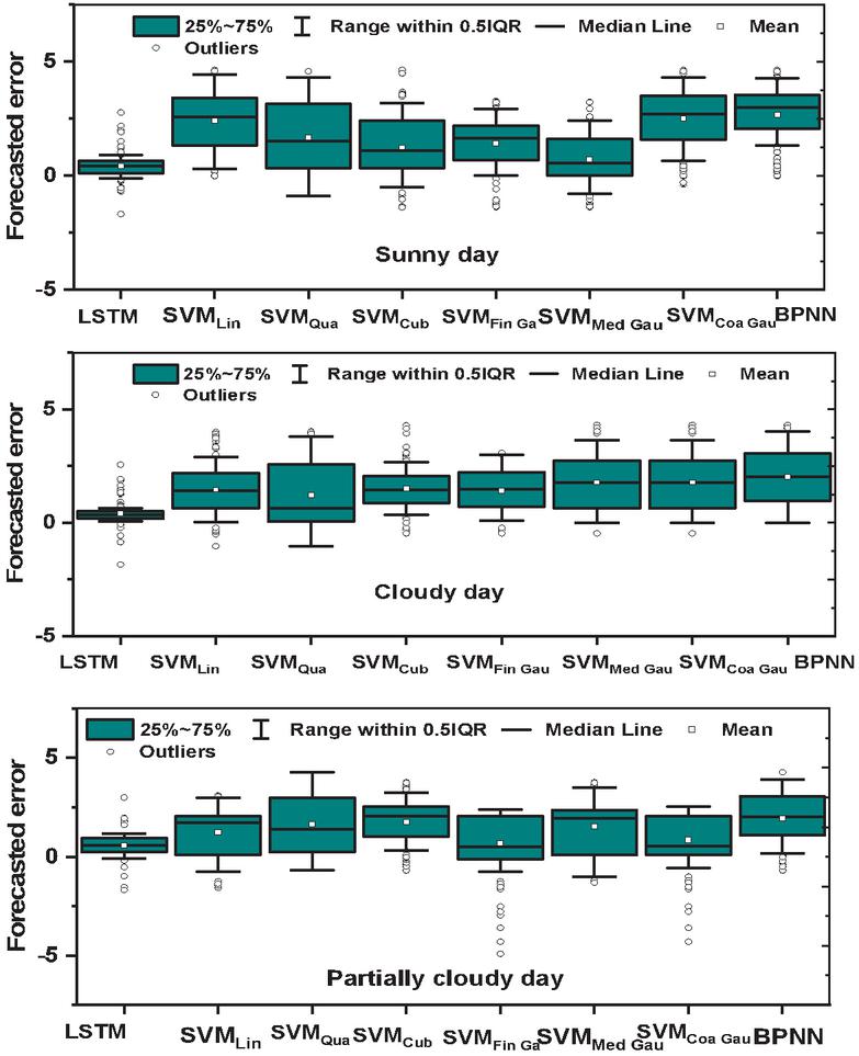
Figure 14 Box plot of forecasted error.
During a sunny, cloudy, and partially cloudy day, the MAE and RMSE values of the LSTM model are 0.35, 0.50, 0.49, and 5.08, 5.71, 5.55, respectively. The estimated MAE and RMSE values of LSTM are better when compared to the MAE and RMSE of the SVM and BPNN algorithms. The LSTM, , and BPNN models can forecast power generation with good accuracy, as shown in Figures 11 and 12. Tables 2 and 3 indicate that the LSTM model outperforms the SVM and BPNN forecasting models. Hence, the LSTM model is fit for power forecasting. Figure 14 depicts box plots of forecasted error versus LSTM, SVM, and BPNN models.
6.1 Diebold-Mariano (DM) Statistical Analysis
Furthermore, the forecasted error of the LSTM, SVM, and BPNN model’s effectiveness is evaluated using the Diebold-Mariano (DM) criterion. The residuals represent the difference between the significance in error measurements of the three forecasts data while comparing with one another such as (LSTM and SVM), (SVM and BPNN), and (LSTM and BPNN). From error data, by using Equations (7)–(11) we can calculate the DM statistical and p-values. The DM and p-values are evaluated according to the absolute error loss.
The order of samples (h) is determined using the equation, ; where n 144. Consider that since , seems to be a suitable value to use after rounding off. Hence, all DM statistics values will be considered for the order h 6. The conditions for the analysis of the significant difference between the two forecasts are:
i. If |DM| and p-value , then there is a substantial variance
ii. If |DM| and p-value , then there is no substantial variance
From Equation (11) by putting we can obtain . The determined DM values and p-values of each weather condition are presented in Table 4.
Following a comparison of LSTM, SVM, and BPNN models, the conclusions can be drawn from Table 4:
1. The DM test based on the absolute error loss suggests that |DM|is greater than for every weather condition considered.
2. Also, it is observed that the p-value is lesser than for every weather condition considered.
Hence, on sunny, cloudy, and partially cloudy days, the |DM| and p-value . So, we can conclude that there is a significant difference between the three forecast models.
Table 4 |DM|and p statistical values
| DM Test Based on LSTM and SVM | DM Test Based on LSTM and BPNN | DM Test Based on SVM and BPNN | |
| |DM| – Sunny day | 3.1751 | 2.8625 | 3.2963 |
| p-value – Sunny day | 0.00149 | 0.00420 | 0.00097 |
| |DM| – Cloudy day | 3.1685 | 2.7082 | 3.0426 |
| p-value – Cloudy day | 0.00153 | 0.00676 | 0.00234 |
| |DM| – Partially cloudy day | 2.6816 | 2.4918 | 1.9698 |
| p-value – Partially cloudy day | 0.00732 | 0.01270 | 0.04886 |
The daily actual and forecasted power of the SOLPSAST system is shown in Figure 15. The SOLPSAST system generates about 80.45 Wh per day on average. The monthly power generation and efficiency of the same are shown in Figure 16. The system efficiency can be calculated using Equation (16). Here, is the system power, A is the area of panels, and n is the number of panels. The average monthly and yearly power generation of the SOLPSAST system is 2.45 kWh and 29.44 kWh respectively.
| (16) |
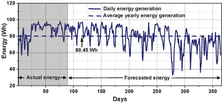
Figure 15 Daily energy generation.
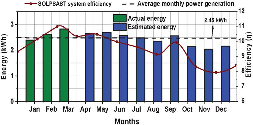
Figure 16 Power generation and efficiency.
7 Conclusion
The proper utilization of solar PV energy set forth future benefits in power system planning applications. The LSTM model is able to forecast the output of SOLPSAST PV power with good accuracy. The resultant performance error indices such as MAE, RMSE, R and MRE for the LSTM model infers that the forecasted output is closer to the actual output power. Furthermore, the significance of the models is analyzed using the Diebold-Mariano test. It is observed from the conditions (|DM| ) and (p-value ) that the three forecasting models are significant for predictive purposes. However, the proposed LSTM model for the SOLPSAST system can be used for future operations. One of the limitations of the LSTM approach is the complexity involved in choosing the right architecture and setting the right control parameters using some statistical approach for the system and data in hand. The non-availability of environmental data such as wind velocity, relative humidity, air temperature, and air pressure definitely reduces the accuracy of the forecast. The reason is that all machine learning algorithms are system or data dependent. However, in future, the environmental parameters which may directly or indirectly effect the forecast output, if considered, will surely improve the performance of the proposed forecast model.
References
[1] Ulyana Koriugina, Daria Illarionova, “Towards Smart Green Cities: Analysis of Integrated Renewable Energy Use in Smart Cities,” Strategic Planning for Energy and the Environment, pp. 75-94, ol. 40, 2021. Available: https://orcid.org/0000-0002-4593-2835
[2] Ninh Nguyen, Thuy Hong Pham, “Promoting Energy Efficiency in an Emerging Market: Insights and Intervention Strategies,” Strategic Planning for Energy and the Environment, pp. 70-80, vol. 38, 2018.
[3] Alkesaiberi, A.; Harrou, F.; Sun, Y. Efficient Wind Power Prediction Using Machine Learning Methods: A Comparative Study. Energies 2022, 15, 2327. Available: https://doi.org/10.3390/en15072327.
[4] Anuj Gupta, Kapil Gupta, Sumit Saroha, “Short Term Solar Irradiation Prediction Framework Based on EEMD-GA-LSTM Method,” Strategic Planning for Energy and the Environment, Vol. 41 Iss. 3, 07–05 2022. Available: https://doi.org/10.13052/spee1048-5236.4132.
[5] Francis M. Lopes, Hugo G. Silva, Rui Salgado, Afonso Cavaco, Paulo Canhoto, Manuel Collares-Pereira, “Short-term forecasts of GHI and DNI for solar energy systems operation: assessment of the ECMWF integrated forecasting system in southern Portugal,” Sol Energy, pp. 14–30, vol. 170, 2018. Available: https://doi.org/10.1016/j.solener.2018.05.039.
[6] J. Alonso-Montesinos, F.J. Batlles, C. Portillo, “Solar irradiance forecasting at one-minute intervals for different sky conditions using sky camera images,” Energy Conversion and Management, pp. 1166–1177, vol. 105, 2015. Available: https://doi.org/10.1016/j.enconman.2015.09.001.
[7] Steven D. Miller, Matthew A. Rogers, John M. Haynes, Manajit Sengupta, Andrew K. Heidinger, “Short-term solar irradiance forecasting via satellite/model coupling,” Solar Energy, pp. 102–117, vol. 168, 2018. Available: https://doi.org/10.1016/j.solener.2017.11.049.
[8] Laith M. Halabi, Saad Mekhilef, Monowar Hossain, “Performance evaluation of hybrid adaptive neuro-fuzzy inference system models for predicting monthly global solar radiation,” Applied Energy, pp. 247–261, vol. 213, 2018. Available: https://doi.org/10.1016/j.apenergy.2018.01.035.
[9] Hou Wei, Xiao Jian, Niu Liyong, “Analysis of power generation capacity of photovoltaic power,” Electr Eng, 2016,17(4):53e8.
[10] Shuwei Miao, Guangtao Ning, Yingzhong Gu, Jiahao Yan, Botao Ma, “Markov Chain model for solar farm generation and its application to generation performance evaluation,” Journal of Cleaner Production, pp. 905–917, vol. 186, 2018. Available: https://doi.org/10.1016/j.jclepro.2018.03.173.
[11] X. G. Agoua, R. Girard and G. Kariniotakis, “Short-Term Spatio-Temporal Forecasting of Photovoltaic Power Production,” IEEE Transactions on Sustainable Energy, pp. 538–546, vol. 9, April, 2018. Available: DOI: 10.1109/TSTE.2017.2747765.
[12] Luca Massidda, Marino Marrocu, “Use of Multilinear Adaptive Regression Splines and numerical weather prediction to forecast the power output of a PV plant in Borkum, Germany,” Solar Energy, pp. 141–149, vol. 146, 2018. Available: https://doi.org/10.1016/j.solener.2017.02.007.
[13] Dairi A, Harrou F, Sun Y, Khadraoui S. “Short-Term Forecasting of Photovoltaic Solar Power Production Using Variational Auto-Encoder Driven Deep Learning Approach” In Applied Sciences, 2020, vol. 10(23), 8400. Available: https://doi.org/10.3390/app10238400.
[14] Anuj Gupta, Kapil Gupta, Sumit Saroha, “Solar Irradiation Forecasting Technologies: A Review,” Strategic Planning for Energy and the Environment, vol. 39, Iss. 3–4, 09-07-2021. Available: https://doi.org/10.13052/spee1048-4236.391413.
[15] Mayur Barman, Nalin Behari Dev Choudhury, “Season specific approach for short-term load forecasting based on hybrid FA-SVM and similarity concept,” Energy, pp. 886–896, vol. 174, 2019. Available: https://doi.org/10.1016/j.energy.2019.03.010.
[16] Jie Shi, Wei-Jen Lee, Yongqian Liu, Yongping Yang and Peng Wang, “Forecasting power output of photovoltaic system based on weather classification and support vector machine,” 2011 IEEE Industry Applications Society Annual Meeting, pp. 1–6, 2011. Available: DOI: 10.1109/IAS.2011.6074294.
[17] Geoffrey K.F. Tso, Kelvin K.W. Yau, “Predicting electricity energy consumption: A comparison of regression analysis, decision tree and neural networks,” Energy, pp. 1761–1768, vol. 32, 2007. Available: https://doi.org/10.1016/j.energy.2006.11.010.
[18] Fermín Rodríguez, Alice Fleetwood, Ainhoa Galarza, Luis Fontán, “Predicting solar energy generation through artificial neural networks using weather forecasts for microgrid control,” Renewable Energy, pp. 855–864, vol. 126, 2018. Available: https://doi.org/10.1016/j.renene.2018.03.070.
[19] Gokhan Mert Yagli, Dazhi Yang, Dipti Srinivasan, “Automatic hourly solar forecasting using machine learning models,” Renewable and Sustainable Energy Reviews, pp. 487–498, vol. 105, 2019. Available: https://doi.org/10.1016/j.rser.2019.02.006.
[20] Adel Mellit, Alessandro Massi Pavan, “A 24-h forecast of solar irradiance using artificial neural network: Application for performance prediction of a grid-connected PV plant at Trieste, Italy,” Solar Energy, pp. 807–821 vol. 84, 2010, Available: https://doi.org/10.1016/j.solener.2010.02.006.
[21] A. Yona, T. Senjyu, A. Y. Saber, T. Funabashi, H. Sekine, C. Kim, “Application of Neural Network to One-Day-Ahead 24 hours Generating Power Forecasting for Photovoltaic System,” 2007 International Conference on Intelligent Systems Applications to Power Systems, pp. 1–6, 2007. Available: DOI: 10.1109/ISAP.2007.4441657.
[22] F. Almonacid, P.J. Pérez-Higueras, Eduardo F. Fernández, L. Hontoria, “A methodology based on dynamic artificial neural network for short-term forecasting of the power output of a PV generator,” Energy Conversion and Management, pp. 389–398, vol. 85, 2014, Available: https://doi.org/10.1016/j.enconman.2014.05.090.
[23] Changsong Chen, Shanxu Duan, Tao Cai, Bangyin Liu, “Online 24-h solar power forecasting based on weather type classification using artificial neural network,” Solar Energy, pp. 2856–2870, vol. 85, Available: https://doi.org/10.1016/j.solener.2011.08.027.
[24] Ercan İzgi, Ahmet Öztopal, Bihter Yerli, Mustafa Kemal Kaymak, Ahmet Duran Şahin, “Short–mid-term solar power prediction by using artificial neural networks,” Solar Energy, pp. 725–733, vol. 86, 2012. Available: https://doi.org/10.1016/j.solener.2011.11.013.
[25] Hugo T.C. Pedro, Carlos F.M. Coimbra, “Assessment of forecasting techniques for solar power production with no exogenous inputs,” Solar Energy, pp. 2017-2028, vol. 86, 2012. Available: https://doi.org/10.1016/j.solener.2012.04.004.
[26] Jie Shi, Wei-Jen Lee, Yongqian Liu, Yongping Yang and Peng Wang, “Forecasting power output of photovoltaic system based on weather classification and support vector machine,” 2011 IEEE Industry Applications Society Annual Meeting, pp. 1–6, 2011. Available: DOI: 10.1109/IAS.2011.6074294.
[27] Monowar Hossain, Saad Mekhilef, Malihe Danesh, Lanre Olatomiwa, Shahaboddin Shamshirband, “Application of extreme learning machine for short term output power forecasting of three grid-connected PV systems,” Journal of Cleaner Production, pp. 395–405, vol. 167, 2017. Available: https://doi.org/10.1016/j.jclepro.2017.08.081.
[28] J. Liu,W. Fang, X. Zhang, and C. Yang, “An improved photovoltaic power forecasting model with the assistance of aerosol index data,” IEEE Trans. Sustain. Energy, pp. 434–442, vol. 6, 2015. Available: DOI: 10.1109/TSTE.2014.2381224.
[29] A. Gensler, J. Henze, B. Sick and N. Raabe, “Deep Learning for solar power forecasting An approach using Auto Encoder and LSTM Neural Networks,” 2016 IEEE International Conference on Systems, Man, and Cybernetics (SMC), 2016, pp. 002858–002865, Available: DOI: 10.1109/SMC.2016.7844673.
[30] W. Lee, K. Kim, J. Park, J. Kim and Y. Kim, “Forecasting Solar Power Using Long-Short Term Memory and Convolutional Neural Networks,” IEEE Access, pp. 73068–73080, vol. 6, 2018. Available: DOI: 10.1109/ACCESS.2018.2883330.
[31] Lee D., Kim K, “Recurrent Neural Network-Based Hourly Prediction of Photovoltaic Power Output Using Meteorological Information,” Energies, 12(2):215, 2019. Available: https://doi.org/10.3390/en12020215.
[32] Abdel-Nasser, M., Mahmoud, K, “Accurate photovoltaic power forecasting models using deep LSTM-RNN,” Neural Comput & Applic 31, pp. 2727–2740 2019. Available: https://doi.org/10.1007/s00521-017-3225-z.
[33] Yoonhwa Jung, Jaehoon Jung, Byungil Kim, SangUk Han, “Long short-term memory recurrent neural network for modeling temporal patterns in long-term power forecasting for solar PV facilities: Case study of South Korea,” Journal of Cleaner Production, p. 119476, vol. 250, 2020. Available: https://doi.org/10.1016/j.jclepro.2019.119476.
[34] Mingming Gao, Jianjing Li, Feng Hong, Dongteng Long, “Day-ahead power forecasting in a large-scale photovoltaic plant based on weather classification using LSTM,” Energy, vol. 187, 2019. Available: https://doi.org/10.1016/j.energy.2019.07.168.
[35] Gao M., Li J, Hong F, Long D, “Short-Term Forecasting of Power Production in a Large-Scale Photovoltaic Plant Based on LSTM,” Applied Sciences, 9(15):3192, 2019. Available: https://doi.org/10.3390/app9153192
[36] F. Mei, “Day-Ahead Nonparametric Probabilistic Forecasting of Photovoltaic Power Generation Based on the LSTM-QRA Ensemble Model,” IEEE Access, pp. 166138–166149, vol. 8, 2020. Available: DOI: 10.1109/ACCESS.2020.3021581.
[37] Kejun Wang, Xiaoxia Qi, Hongda Liu, “Photovoltaic power forecasting-based LSTM-Convolutional Network,” Energy, vol. 189, 2019. Available: https://doi.org/10.1016/j.energy.2019.116225.
[38] Wang Fei, Zhiming Xuan, Zhao Zhen, Kangping Li, Tieqiang Wang, Min Shi. “A day-ahead PV power forecasting method based on LSTM-RNN model and time correlation modification under partial daily pattern prediction framework,” Energy Conversion and Management, 212, 2020. Available: https://doi.org/10.1016/j.enconman.2020.112766
[39] Chen B, Lin P, Lai Y, Cheng S, Chen Z, Wu L. “Very-Short-Term Power Prediction for PV Power Plants Using a Simple and Effective RCC-LSTM Model Based on Short Term Multivariate Historical Datasets,” Electronics, 2020. Available: https://doi.org/10.3390/electronics9020289
[40] K. Kumba, S. P. Simon, K. Sundareswaran, P. S. R. Nayak, K. A. Kumar and N. P. Padhy, “Performance Evaluation of a Second-Order Lever Single Axis Solar Tracking System,” IEEE Journal of Photovoltaic, Vol. 12, Issue: 5, pp. 1219–1229, 23/06/2022. Available: https://ieeexplore.ieee.org/document/9828802
[41] Harrou, Fouzi, Kadri, Farid, Sun, Ying. “Forecasting of Photovoltaic Solar Power Production Using LSTM Approach” In Advanced Statistical Modeling, Forecasting, and Fault Detection in Renewable Energy Systems, edited by Fouzi Harrou, Ying Sun. London: Intech Open, 2020. Available: Doi: 10.5772/intechopen.91248.
[42] MathWorks, http://www.mathworks.com (2020).
[43] R. Jiao, T. Zhang, Y. Jiang, H. He, “Short-term non-residential load forecasting based on multiple sequences LSTM recurrent neural network,” IEEE Access, pp. 59438–59448, vol. 6, 2018. Available: DOI: 10.1109/ACCESS.2018.2873712.
[44] G. Chicco, V. Cocina, P. Di Leo, F. Spertino, A. Massi Pavan, “Error assessment of solar irradiance forecasts and AC power from energy conversion model in grid-connected photovoltaic systems,” Energies, vol. 9, no. 1, p. 8, 2015. Available: https://doi.org/10.3390/en9010008
[45] M. A. E. Bhuiyan, F. Yang, N. K. Biswas, S. H. Rahat, T. J. Neelam, “Machine learning-based error modeling to improve GPM IMERG precipitation product over the Brahmaputra river basin,” Forecasting, pp. 248–266, Vol. 2, 2020. Available: https://doi.org/10.3390/forecast2030014
[46] Diebold F.X., Mariano R., “Comparing predictive accuracy,” J. Bus. Econ. Stat., 1995, 13, 253–265.
[47] Diebold F.X., “Element of Forecasting,” 4 ed., Thomson South-western: Cincinnati, OH, USA, 2007, pp. 257–287.
Biographies

Krishna Kumba received the B.Tech. degree in electrical and electronics engineering from JNTU Hyderabad, India, in 2008; and the M. Tech. degree in the control system, from the National Institute of Technology Kurukshetra, Haryana, India, in 2010. Currently, he is pursuing a Ph.D. degree in electrical and electronics engineering from the National Institute of Technology, Tiruchirappalli, Tamil Nadu, India. His research interests include power system planning and reliability. renewable energy systems.

Sishaj P. Simon was born in India. He received a B.Eng. degree in electrical and electronics engineering, an M.Eng. degree in applied electronics both from Bharathiar University, Coimbatore, Tamil Nadu, India, in 1999 and 2001, respectively, and a Ph.D. degree in power system engineering from the Indian Institute of Technology (IIT), Roorkee, Uttarakhand, India, in 2006. Currently, he is an Associate Professor with the Department of Electrical and Electronics Engineering, National Institute of Technology (NIT) (formerly Regional Engineering College), Tiruchirappalli, Tamil Nadu, India. His research interests include the area of power system operation and control, power system planning and reliability, artificial neural networks, fuzzy logic systems, and the application of meta-heuristics, and intelligent techniques to power systems.

Kinattingal Sundareswaran was born in Pallassana, Kerala, India, in 1966. He received the B.Tech. (Hons.) degree in electrical and electronics engineering and the M.Tech. (Hons.) degree in power electronics from the University of Calicut, Calicut, Kerala, India, in 1988 and 1991, respectively, and the Ph.D. degree in electrical engineering from Bharathidasan University, Tiruchirappalli, Tamil Nadu, India, in 2001. From 2005 to 2006, he was a professor with the Department of Electrical Engineering, National Institute of Technology, Calicut, Kerala, India. He is currently a Professor with the Department of Electrical and Electronics Engineering, National Institute of Technology, Tiruchirappalli, Tamil Nadu, India. His research interests include power electronics, renewable energy systems, and biologically inspired optimization techniques.

Panugothu Srinivasan Rao Nayak was born in Perikapadu, Guntur, Andhra Pradesh, India, in 1979. He received the B.Tech. degree in electrical and electronics engineering from Bapatla Engineering College (BEC), Bapatla, Guntur, in 2001; the M.Tech. degree in energy systems from Jawaharlal Nehru Technological University (JNTU), Hyderabad, Telangana, India, in 2006; and the Ph.D. degree in electrical engineering from the National Institute of Technology, Tiruchirappalli, Tamil Nadu, India, in 2014. Currently, he is an Assistant Professor with the Department of Electrical and Electronics Engineering, National Institute of Technology. His research interests include power electronics and drives, biologically inspired optimization techniques, and wireless power transfer systems
Strategic Planning for Energy and the Environment, Vol. 42_2, 375–404.
doi: 10.13052/spee1048-5236.4226
© 2023 River Publishers