Setting Up Optimal Meteorological Networks: An Example From Italy

Rita Aromolo^*, Valerio Moretti and Tiziano Sorgi

Council for Agricultural Research and Economics (CREA), Rome, Italy

E-mail: rita.aromolo@crea.gov.it

*Corresponding Author

Received 18 July 2021; Accepted 21 July 2021; Publication 05 October 2021

Abstract

A permanent assessment of climate regime in forest sites has a key role in forest resource conservation and preservation of ecosystem services, biodiversity and landscape multi-functionality, informing sustainable forest management. In this view, time-series of meteorological data relative to several monitoring sites from the ICP-Forest network in Italy, were analyzed with the aim to define the number of site-specific observations, which can be considered adequate for further analysis on forest resource management. The relative importance of each factor accounted in our analysis (season, year, variable, plot, sampling proportion) was investigated comparing results through the use of descriptive statistics.

Keywords: Climate, gauging stations, descriptive statistics, Mediterranean Europe.

Introduction

A permanent assessment of climate regime in forest sites has a key role in forest resource conservation and preservation of ecosystem services, biodiversity and landscape multi-functionality, informing sustainable forest management (Marchetti et al. 2014, Salvati et al. 2016). In this view, time-series of meteorological data relative to several monitoring sites from the ICP-Forest network in Italy, were analyzed with the aim to define the minimum number of site-specific observations, which can be considered adequate for further analysis on forest resource management (Marchi et al. 2017). for each recorded variable, missing values were filled by using a multivariate Singular Value Decomposition (SVD) imputation. A decreasing number of records were progressively removed using a bootstrap repetition following evaluation of the representativeness of the remained records in terms of error of estimation and explained variance on the whole climatic period. Moreover, the relative importance of each factor accounted in our analysis (season, year, variable, plot, sampling proportion) was investigated fitting a model on the results of the overall procedure.

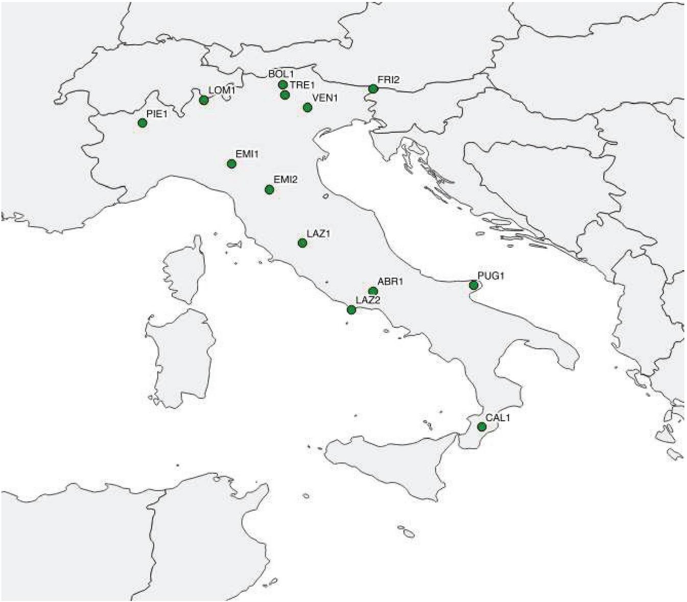
Figure 1 Spatial distribution of the monitoring sites.

Methodology

The climatic data derives form the data logger installed at 13 selected areas: ABR 1 Selva Piana; CAL 1 Piano Limina; EMI 1 Carrega; LAZ 1 Monte Rufeno; PIE 1 Valsessera; VEN 1 Pian Cansiglio; EMI 2 Brasimonte; FRI 2 Tarvisio; LOM 1 Val Masino; PUG 1 Foresta Umbra; TRE 1 Passo Lavaz ; LAZ 2 Monte Circeo; BOL 1 Renon (Figure 1). The detected variables, monitored over multiple annual cycles, are air temperature for the profile of 0.1 m and 2 m (AT01 and AT2), relative humidity for the profile of 0.1 m and 2 m (RH01 and RH2), and precipitation (PR). The data time lapse is 1th January 1998–31th December 2013, with 1-day sampling interval. The daily data has been obtained from the average of each performed scan (sensors scan frequency is 10 seconds) for each examined variable, except for the precipitation, which derives from the measurements sum.

Results and Discussion

Results are reported in the following tables and figures.

Table 1 Description of the analyzed time period, including the available years number of monitoring (N years), the starting and ending date, the valid and missing values number over a total of 5844 observations, calculated for each variable, relative to 13 selected meteorological stations

Stations	Statistics	AT01	AT2	RH01	RH2	PR
01-ABR1	N years	4	16	4	16	16
	Starting date	01/01/1998	01/01/1998	01/01/1998	01/01/1998	01/01/1998
	Ending date	26/11/2001	31/12/2013	26/10/2001	31/12/2013	31/12/2013
	N valid data	1215	4473	4242	981	4178
	N missing data	4629	1371	4863	1666	1602
03-CAL1	N years	12	12	12	12	12
	Starting date	01/05/1999	01/05/1999	01/05/1999	01/05/1999	01/05/1999
	Ending date	26/07/2010	26/07/2010	26/07/2010	26/07/2010	26/07/2010
	N valid data	2997	2949	2977	2997	2991
	N missing data	2847	2895	2847	2853	2867
05-EMI1	N years	16	16	16	16	16
	Starting date	01/01/1998	01/01/1998	01/01/1998	01/01/1998	01/01/1998
	Ending date	14/10/2013	14/10/2013	14/10/2013	14/10/2013	14/10/2013
	N valid data	5698	5698	5726	5722	5722
	N missing data	146	146	122	122	118
09-LAZ1	N years	16	16	16	16	16
	Starting date	01/01/1998	01/01/1998	01/01/1998	01/01/1998	01/01/1998
	Ending date	29/12/2013	29/12/2013	29/12/2013	29/12/2013	29/12/2013
	N valid data	5532	5531	5582	5535	5567
	N missing data	312	313	309	277	262
12-PIE1	N years	14	14	14	14	14
	Starting date	01/11/1999	01/11/1999	01/11/1999	01/11/1999	01/11/1999
	Ending date	12/11/2012	12/11/2012	12/11/2012	12/11/2012	12/11/2012
	N valid data	4130	4130	4188	4130	4130
	N missing data	1714	1714	1714	1714	1656
20-VEN1	N years	15	15	15	15	15
	Starting date	01/08/1999	01/08/1999	01/08/1999	01/08/1999	01/08/1999
	Ending date	31/12/2013	31/12/2013	31/12/2013	31/12/2013	31/12/2013
	N valid data	4799	4982	4933	4812	4916
	N missing data	1045	862	1032	928	911
06-EMI2	N years	11	11	10	11	11
	Starting date	20/10/1998	20/10/1998	09/06/1999	20/10/1998	20/10/1998
	Ending date	31/12/2008	31/12/2008	31/12/2008	31/12/2008	31/12/2008
	N valid data	3172	3205	3479	2840	3082
	N missing data	2672	2639	3004	2762	2365
08-FRI2	N years	15	15	15	15	15
	Starting date	05/06/1998	05/06/1998	05/06/1998	05/06/1998	05/06/1998
	Ending date	04/04/2012	04/04/2012	04/04/2012	04/04/2012	04/04/2012
	N valid data	4801	4801	4773	4801	4558
	N missing data	1043	1043	1043	1286	1071
10-LOM1	N years	–	10	–	10	10
	Starting date	–	16/04/2003	–	16/04/2003	16/04/2003
	Ending date	–	04/11/2013	–	04/11/2013	04/11/2013
	N valid data	–	2383	2052	–	2383
	N missing data	5844	3461	5844	3461	3792
13-PUG1	N years	–	5	–	5	5
	Starting date	–	28/05/2009	–	28/05/2009	28/05/2009
	Ending date	-	31/12/2013	–	31/12/2013	31/12/2013
	N valid data	–	1608	1610	–	1608
	N missing data	5844	4236	5844	4236	4234
17-TRE1	N years	16	16	16	16	16
	Starting date	17/09/1998	17/09/1998	17/09/1998	17/09/1998	17/09/1998
	Ending date	07/04/2013	26/10/2001	07/04/2013	07/04/2013	26/10/2001
	N valid data	5205	5205	5082	5205	5205
	N missing data	639	639	639	639	762
22-LAZ2	N years	–	8	–	8	8
	Starting date	–	27/07/2005	–	27/07/2005	27/07/2005
	Ending date	–	27/06/2012	–	27/06/2012	27/06/2012
	N valid data	–	2458	2458	–	2457
	N missing data	5844	3386	5844	3387	3386
27-BOL1	N years	–	9	–	4	9
	Starting date	–	11/02/2004	–	17/09/2004	07/01/2004
	Ending date	–	07/11/2012	–	31/12/2007	31/12/2007
	N valid data	–	2658	1144	–	2798
	N missing data	5844	3186	5844	3046	4700

Table 2 Summary statistics, including the mean and median, standard deviation and coefficient of variation values, calculated for each variable, relative to 13 selected sites during the entire analyzed time period. Note that the variation coefficient (CV) is a dimensionless quantity

Stations	Statistics	AT01 (${}^{\circ }$C)	AT2 (${}^{\circ }$C)	RH01 (%)	RH2 (%)	PR (mm)
01-ABR1	Mean	6.63	7.21	79.62	83.12	2.06
	Median	7.1	7.6	82.1	86.4	0
	Std Dev	6.66	6.74	16.49	15.87	6.61
	CV	100.5	93.48	20.71	19.1	320.65
03-CAL1	Mean	10.83	11	89.17	86.4	3.91
	Median	10.8	11	95.5	93	0
	Std Dev	6.23	6.24	13.87	15.64	10.22
	CV	57.53	56.71	15.56	18.1	261.12
05-EMI1	Mean	12.22	12.02	81.16	80.64	1.92
	Median	12.5	12.3	84.75	85.2	0
	Std Dev	8.17	8.06	17.28	18.37	6.1
	CV	66.89	67.03	21.29	22.78	318.06
09-LAZ1	Mean	11.25	11	79.63	75.62	2.51
	Median	11.1	10.6	82	78.2	0
	Std Dev	7.3	6.92	15.18	17.51	6.99
	CV	64.86	62.93	19.06	23.16	279.01
12-PIE1	Mean	6.09	7.31	85.94	79.27	4.54
	Median	6.1	7.3	93.9	84.9	0
	Std Dev	6.96	6.82	17.23	20.1	15.52
	CV	114.35	93.19	20.05	25.35	341.81
20-VEN1	Media	4.5	5.72	91.34	85.75	4.72
	Median	4.8	6	93.4	90.1	0
	Dev std	7.28	7.2	8.98	14.2	13.85
	CV	161.67	125.89	9.83	16.56	293.21
06-EMI2	Mean	9.8	9.54	82.07	80.06	3.64
	Median	10	9.3	85.9	84.2	0
	Std Dev	7	7.03	16.36	17.36	9.95
	CV	71.45	73.67	19.94	21.69	273.66
08-FRI2	Mean	6.16	5.91	92.63	91.36	3.62
	Median	6.6	6.3	96.3	95.5	0
	Std Dev	7.56	7.64	8.79	10.89	11.05
	CV	122.7	129.15	9.49	11.92	305.05
10-LOM1	Mean	–	7.55	–	71.1	2.96
	Median	–	8.2	–	73	0
	Std Dev	–	6.71	–	17.34	8.13
	CV	–	88.82	–	24.38	274.13
13-PUG1	Mean	–	11.91	–	78.7	2.09
	Median	–	11.7	–	83	0
	Std Dev	–	6.87	–	13.71	6.99
	CV	–	57.71	–	17.41	334.7
17-TRE1	Mean	1.8	2.21	94.8	86.39	2.19
	Median	1.1	2	99.7	91.2	0
	Std Dev	7.24	7.29	9	14.44	5.89
	CV	401.24	330.18	9.49	16.71	268.88
22-LAZ2	Mean	–	15.72	–	77.42	1.3
	Median	–	15.3	–	79	0
	Std Dev	–	5.96	–	12.34	4.43
	CV	–	37.9	–	15.94	340.25
27-BOL1	Mean	–	4.45	–	72.75	3.01
	Median	–	4.7	–	75	0
	Std Dev	–	6.91	–	18.04	8.91
	CV	–	155.35	-	24.79	295.97

The presence of missing values in a data set can affect the conclusions made using the data. Missing data values must not only be identified, they must also be understood before further analysis can be conducted.

The data filling analysis can be useful for prevention and treatment of missing data. A multivariate Singular Value Decomposition (SVD) imputation has been used to simulate missing values. The algorithm commonly known as Principal Component Analysis (PCA), for instance, is just a simple application of the SVD. In this method, the SVD is used to obtain a set of orthogonal vectors that are linearly combined to estimate missing data values; this procedure is repeated until it converges and the convergence depends on the configuration of the missing entries. The fact that SVD gives us an optimal low-rank representation guarantees that this sort of simulation preserves most of the detail in the data matrix. The time series data analyses relevant to each analyzed variable in the 13 selected sites have been explored to cross-validate the SVD imputation. Figure 3 depicts both the source and implemented time series data analyses relevant to each analyzed variable in all the stations, as a representative example for all stations.

The time series trend analysis has also been performed to verify if there is a linear long-term increase or decrease in both the source and filled data (Table 3).

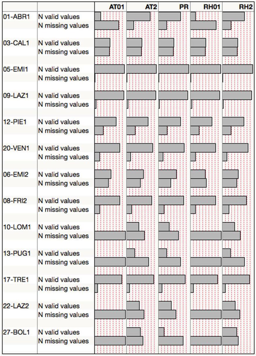
Figure 2 Number of valid and missing values, calculated for each variables, relative to 13 selected sites during the entire analyzed time period.

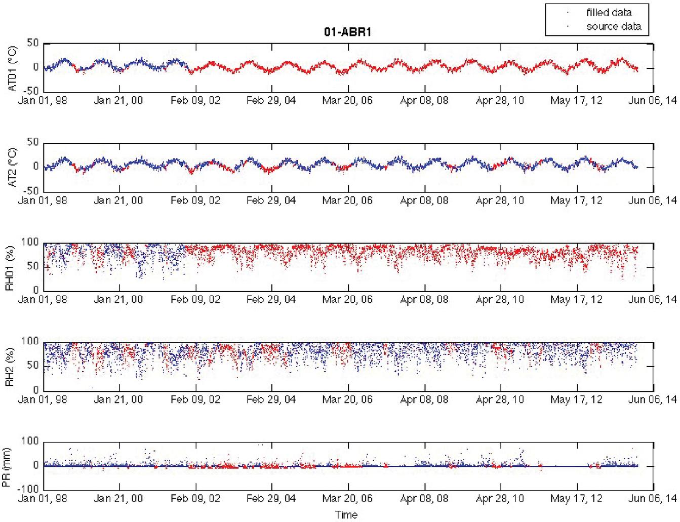
Figure 3 Meteorological time series of air temperature (0.1 and 2 m), relative humidity (0.1 and 2 m), and precipitation, as recorded at ABR1 station during the considered time period. The source data are represented by blue points, the simulated data by red ones.

Table 3 The source/filled time series linear trend parameters, calculated for each analyzed variable in all the stations

Source Data
	AT01		AT2		RH01		RH2		PR
	Slope	Intercept	Slope	Intercept	Slope	Intercept	Slope	Intercept	Slope	Intercept
Station	(${}^{\circ }$C year${}^{-1}$)	(${}^{\circ }$C)	(${}^{\circ }$C year${}^{-1}$)	(${}^{\circ }$C)	(${}^{\circ }$C year${}^{-1}$)	(${}^{\circ }$C)	(${}^{\circ }$C year${}^{-1}$)	(${}^{\circ }$C)	(${}^{\circ }$C year${}^{-1}$)	(${}^{\circ }$C)
‘01-ABR1’	7,35E-01	5,16	2,53E-02	7,00	$-$2,22E+00	84,11	8,25E-01	76,38	$-$3,37E-02	2,34
‘03-CAL1’	$-$9,26E-02	11,44	$-$9,94E-02	11,65	3,86E-01	86,62	6,75E-01	81,95	8,13E-02	3,37
‘05-EMI1’	2,50E-02	12,02	$-$9,05E-03	12,09	7,30E-01	75,39	5,15E-03	80,60	$-$1,96E-03	1,93
‘09-LAZ1’	1,99E-01	9,72	1,04E-02	10,92	$-$4,63E-01	83,23	$-$3,70E-01	78,49	6,16E-02	2,03
‘12-PIE1’	9,42E-03	6,01	1,20E-01	6,34	1,01E+00	77,70	1,09E+00	70,35	$-$9,70E-02	5,33
‘20-VEN1’	$-$1,72E-02	4,65	9,56E-02	4,89	$-$4,29E-01	95,05	$-$1,42E+00	97,90	$-$1,64E-02	4,87
‘06-EMI2’	4,49E-01	7,22	2,18E-01	8,30	1,30E-01	81,26	$-$1,67E-01	81,02	$-$4,15E-02	3,88
‘08-FRI2’	$-$6,18E-02	6,61	$-$1,78E-01	7,21	4,20E-01	89,57	6,96E-01	86,24	$-$2,10E-01	5,15
‘10-LOM1’	$-$	$-$	$-$2,36E-01	9,80	$-$	$-$	1,44E+00	57,36	$-$1,18E-01	4,14
‘13-PUG1’	$-$	$-$	$-$3,32E-02	12,37	$-$	$-$	1,76E-02	78,46	$-$1,80E-01	4,56
‘17-TRE1’	$-$1,19E-01	2,74	$-$7,87E-02	2,83	8,49E-01	88,12	2,35E-01	84,54	$-$4,62E-02	2,56
‘22-LAZ2’	$-$	$-$	$-$5,53E-02	16,33	$-$	$-$	$-$4,10E-01	81,95	$-$1,86E-01	3,35
‘27-BOL1’	$-$	$-$	1,92E-01	2,46	$-$	$-$	$-$5,05E-01	78,32	$-$1,47E+00	15,34
‘01-ABR1’	$-$7,93E-03	3,68	1,60E-01	4,64	$-$1,98E-01	82,06	8,55E-01	75,51	4,07E-02	0,46
‘03-CAL1’	1,55E-02	11,63	4,56E-01	10,43	$-$2,22E-02	89,81	7,91E-01	81,14	2,97E-01	5,72
‘05-EMI1’	2,32E-02	11,90	1,79E-02	11,84	7,13E-01	75,49	5,25E-02	80,25	2,29E-02	1,83
‘09-LAZ1’	2,53E-01	9,46	7,99E-02	10,65	$-$4,47E-01	83,05	$-$3,14E-01	78,13	8,75E-02	1,92
‘12-PIE1’	$-$2,26E-01	7,52	5,82E-02	7,08	9,50E-01	77,35	8,23E-01	72,12	$-$3,78E-02	4,99
‘20-VEN1’	$-$2,65E-02	4,93	7,55E-02	5,15	$-$6,01E-02	91,52	$-$7,74E-01	91,54	7,56E-02	3,75
‘06-EMI2’	9,60E-02	8,84	1,64E-01	8,94	2,11E-02	80,99	$-$4,82E-02	79,04	$-$1,51E-01	3,54
‘08-FRI2’	3,92E-02	6,61	4,44E-02	6,10	3,00E-01	90,34	2,64E-01	88,33	$-$9,54E-02	4,41
‘10-LOM1’	$-$1,96E-01	3,33	1,29E-01	3,84	7,91E-01	64,37	8,70E-01	60,67	$-$1,15E-02	1,77
‘13-PUG1’	7,39E-02	5,47	4,31E-01	4,49	$-$6,03E-02	74,93	4,46E-01	72,89	1,89E-01	$-$1,50
‘17-TRE1’	$-$3,45E-02	2,78	4,68E-02	2,69	6,75E-01	88,78	2,92E-01	84,07	1,23E-02	1,93
‘22-LAZ2’	9,04E-02	7,76	4,97E-01	7,92	$-$1,63E-01	74,66	6,45E-01	69,23	3,15E-02	1,22
‘27-BOL1’	$-$1,06E-01	5,08	$-$2,37E-02	5,23	4,11E-01	75,18	1,32E-01	70,93	$-$6,88E-02	4,91

Conclusions

The climatic data, collected in the 16-year period (1998–2013), has been evaluated as a part of the SMART4Action Project. The integration of climate impact assessment into the forest response is fundamental to achieve sustainable forest management. The climatic data derives form a monitoring network composed by 13 test sites. In particular, the analyzed variables, detected in each site, are air temperature and relative humidity for the profile of 0.1 m and 2 m and precipitation. Time series represent the time-evolution of the meteorological dynamic process and are used to evaluate patterns and behavior in data over time and to examine daily, weekly, seasonal or annual variations, or before-and-after effects of a process change. This data has been used to provide an overview of the climatic conditions of the tested areas, including a summary statistics of the measured variables in each provided sites and their time-evolution. Moreover, once defined the number of valid and missing values, a data filling analysis has been performed to obtain useful information for prevention and treatment of missing data. To check whether a linear long-term increase or decrease occurs in both source and filled data, a time series trend analysis has also been performed. The source and simulated results comparison has revealed that a proper data filling procedure can be used when valid data are not available.

References

Bertini G., Amoriello T., Fabbio G., Piovosi M., 2011. Forest growth and climate change. Evidences from the ICP-Forests intensive monitoring in Italy. iForest 4: 262–267.

Breiman L (2001). Random forests. Machine learning 5–32. doi: 10.1023/A:1010933404324

Fabbio G, Merlo M, Tosi V., 2003. Silvicultural management in maintaining biodiversity and resistance of forests in Europe—the Mediterranean region. Journal of Environmental Management 67: 67–76.

Fares S., Mugnozza G. S., Corona P., Palah M., 2015. Sustainability: Five steps for managing Europe’s forests. Nature 519 (7544): 407–409.

Ferrara C., Marchi M., Fares S., Salvati, L., 2017. Sampling strategies for high quality time-series of climatic variables in forest resource assessment. iForest, underlineaccepted.

Ferretti M., Fischer R., editors, 2013. Forest Monitoring, Vol 12, DENS, UK: Elsevier, 2013, 507 ps.

Golub G. and Kahan W., 1965. Calculating the singular values and pseudo-inverse of a matrix, J. Soc. Indust. Appl. Math. Ser. B Numer. Anal., 2: 205–224.

Jump S.A., Penuelas J., 2005. Running to stand still: adaptation and the response of plants to rapid climate change. Ecology Letters 8: 1010–1020.

Lindner M., Maroschek M., Netherer S., Kremer A., Barbati A., Garcia-Gonzalo J., Seidl R., Delzon S., Corona P., Kolstroma M., Lexer MJ., Marchetti M., 2010. Climate change impacts, adaptive capacity, and vulnerability of European forest ecosystems. Forest Ecology and Management 259: 698–709.

Marchetti M, Vizzarri M, Lasserre B, Sallustio L, Tavone A (2014). Natural capital and bioeconomy?: challenges and opportunities for forestry. Annals of Silvicultural Research 38:62–73. doi: 10.12899/ASR-1013.

Marchi M, Ferrara C, Bertini G, Fares S, Salvati L (2017b). A sampling design strategy to reduce survey costs in forest monitoring. Ecological Indicators 81:182–191. doi: 10.1016/j.ecolind.2017.05.011

R Core Team (2017). R: a language and environment for statistical computing. R Foundation for Statistical Computing, Vienna, Austria. URL https://www.R-project.org/.

Salvati L, Becagli C, Bertini G, Cantiani P, Ferrara C, Fabbio G (2016). Toward sustainable forest management indicators? A data mining approach to evaluate the impact of silvicultural practices on stand structure. International Journal of Sustainable Development & World Ecology 0:1–11. doi: 10.1080/13504509.2016.1239138

Scheick J.T., Linear algebra with applications, McGraw-Hill, New York, 1996.

Travaglini D., Chirici G., Bottalico F., Ferretti M., Corona P., Barbati A., Fattorini F., 2013. Large-Scale Pan-European Forest Monitoring Network: A Statistical Perspective for Designing and Combining Country Estimates. Example for Defoliation. In Marco Ferretti, Richard Fischer, editors: Forest Monitoring, Vol 12, DENS, UK: Elsevier, 2013, pp. 105–136.

Biographies

Rita Aromolo – Senior Technologist, degree in Biological Sciences from the La Sapienza University of Rome and specialization in General Pathology. Since 1988 she has been working for the Council for Agricultural Research and Analysis of the Agricultural Economy at Center of Agriculture and Environment. She carries out research in the study and analysis of heavy metals in soil and plants, chemical indicators of soil fertility in assessing the environmental impact, the influence of cultivation practices on product quality and chemical characteristics physics of soils, air pollution and environmental quality. Responsible for various research also in the context of Mipaaf projects, the most recent “Valorbio”, Agroener, and thesis co-supervisor in the degree course in Forestry Sciences of the University of Tuscia of Viterbo. Since 1996 she has been responsible for various conventions in the environmental monitoring of the Presidential Estate of Castelporziano. She cooperates in various research projects such as projects aimed at optimizing fertilization through the use of biomass of various kinds on crops for industrial use, for the agricultural enhancement of waste biomass, and for the effects of the dynamics of unwanted elements on the soil. Since 2014 She has been working as an expert in the scientific technical group set up by interministerial decree as part of the investigations on the Terra dei Fuochi. She is the author of over 140 scientific publications and two patents.

Valerio Moretti, born in Rome on 16/12/1980. In 1999 he obtained a scientific high school diploma and subsequently began working at CREA in the context of national projects for the environmental protection of the Presidential Estate of Castelporziano. Since 2016 he has been dealing with the management of European projects both for the technical and administrative aspects. The most relevant technical tasks are the installation of weather stations in Italy and the implementation of climate databases.

Tiziano Sorgi, born in Rome on 24/07/1974. In 1993 he graduated as a technician of the electrical and electronic industries with a score of 60/60 and subsequently obtained a diploma of hardware and software technician with a score of 30/30. In 1998 he was hired at CREA where he is currently employed as a computer technician and electronic technician; among the most important tasks are the installation of meteorological stations on the Italian territory, the management of climate databases and the wiring of electronic instruments to the relative acquisition devices. The passion for electronics and for the computer led him to implement the design of interfaces and devices through the use of Arduino and the knowledge of the Visual C$++$ programming language.

Strategic Planning for Energy and the Environment, Vol. 40_1, 39–54.
doi: 10.13052/spee1048-5236.4013
© 2021 River Publishers

Abstract

Introduction

Methodology

Results and Discussion

Conclusions

References

Biographies