Passenger Transport Modal Mix by Incorporating Travel Behaviour: A Case Study of Kathmandu Valley, Nepal
Anita Prajapati*, Nawraj Bhattarai and Tri Ratna Bajracharya
Department of Mechanical and Aerospace Engineering, Pulchowk Campus, Institute of Engineering, Tribhuvan University, Pulchowk, Lalitpur, Nepal
E-mail: anita.praj@pcampus.edu.np; bnawraj@ioe.edu.np; triratna@ioe.edu.np
*Corresponding Author
Received 29 September 2021; Accepted 24 November 2021; Publication 14 December 2021
Abstract
Most of the travel demand in developing countries is fulfilled by private vehicles dominated by 2-wheelers due to their affordability, accessibility, and availability, which has direct effects on energy, economy, and environment. To achieve sustainable transport, policies such as electric mobility and mass transport options have been implemented which are mainly focused on technology shift based on technology cost and environmental externalities. Transport modelling in this study was carried out using an additional attribute: travel time which shows the impact of travel behaviour on the optimal modal mix and the consequent impact on energy and emissions. The scenario-based approach using the travel time budget (TTB) concept was used using a bottom-up TIMES modelling framework. The scenario analysis shows the trade-off between the speed of the vehicle, available travel time, and sustainability in transport. The result suggests that the investment in rapid transit would be the potential future mode in Kathmandu valley.
Keywords: Travel behaviour, TIMES model, travel time, energy, emissions.
1 Introduction
The transport sector plays an important role in boosting the economy through the passengers as well as freights movement. Exceeding consumption of petroleum products has been its major issue due to depleting non–renewable sources as well as exhaust emissions. Globally, 59% of the total end-use sector liquid-fuels are consumed in the transport sector in 2018 [1]. Motor gasoline dominates the other fuels accounting for 35% of the world’s transportation-related energy use. It was estimated that this sector consumed approximately 26% of total world energy, increasing annually at the rate of 1.8% per annum during 2010–2018 [1]. Due to slower economic progress, low population growth, and improving fuel economy, the petroleum consumption is decreasing in OECD countries compared to Non-OECD countries where Light-Duty Vehicles (LDVs) are increasing rapidly at the rate of 6% per annum during 2010–2018, mostly in countries like China, India and other Asian countries. Due to the slow progression to electric vehicles, only 25% of the total LDVs are expected to be electric, and more than 50% of motor gasoline vehicles to dominate by 2050 [1]. In a path to cleaner fuels in transportation, the Global Fuel Economy Initiatives (GFEI) has also endorsed the target of improving fuel efficiency by 50% by 2050 from 2005 level, primarily by shifting to electric vehicles and improving the fuel economy of LDVs [2]. Dependency on fossil fuels, growing transport-related emissions, and increasing transport activities are the major concerns in the transport sector, where countries are striving towards sustainability as indicated by the Sustainable Development Goals (SDGs). The annual travel demand is increasing at the rate of 4% in Non-OECD countries, from 2400 km/capita to 4600 km/capita during 2000–2015 [3]. The global modal mix scenario also shows that 52% of travel demand is contributed by passenger cars, 34% by public bus, and 15% by two and three-wheelers in 2015. The contrasting mix in OECD and Non-OECD countries for passenger cars is 84% and 37% and that for 2-wheelers is 3% and 19% respectively. Among the Non-OECD countries, China and India dominate the total transport demand, which is even expected to rise to 43% of the world’s transportation demand by 2050 as per the International Transport Forum. The transport modal mix in South-East Asia also shows the tremendous growth in both 2-wheelers and 4 wheelers, mostly the former in low per capita income countries and later in advanced economy countries [4]. Due to easy access, affordability, and convenience for a short distance of 2-wheelers, and poor infrastructures for 4-wheelers, the ownership rate of 2-wheelers is high and common among low and middle-income countries [5]. In Both cases, there is the accelerated growth of private vehicles than public vehicles, which increases not only energy consumptions and emissions but also congestions.
To understand the future transport scenario, a modelling approach that resembles the real transport scenario is vital. There is a substantial preference for a bottom-up approach in transport energy planning due to its flexibility and robust representation of the existing transport systems [6]. Most of the transport modelling are carried out focusing on reducing energy and emissions for sustainable transport planning. However, it is also critical to incorporate the travel behaviour in modelling transport modal mix as the modal shift is dependent on how user’s mode choice as well. Meanwhile, Venturini [6] also indicated that the bottom-up model in the transport model is suitable when incorporating the travel behaviour by linking the model with an external transport simulation model. The simulation is carried out to project travel demand exogenously which is influenced by variables such as urbanization rate, per capita income, and population growth rate.
In a technology choice model that includes adequate data on technical, environmental, and economic characteristics, the inclusion of non-monetary parameters that affect consumers’ decisions is also vital. Due to the complexity in utilization patterns of individual technologies, unique operating parameters, and consumer preference of individual modes the evaluation of energy consumption for transport technologies in transport modes has become complex [7]. The five major behavioural features to include behaviour in energy and transport systems, as reviewed by [6] are technology choice, modal choice, driving patterns, and new mobility trend, the first two being the most effective. Representing travel behaviour in the energy system is broad yet vital due to its importance in integrated future energy planning systems [8]. The most used methodologies to represent technology choice with behaviour inclusion are discrete choice models, constant elasticities of substitutions, disutility costs, and hurdle rates [6]. The disutility costs function considers the discomfort cost of users when shifting from one technology to another. A linear programming model using TIMES/MESSAGE has been used to represent the disutility cost functions. The disutility costs reflect that different transport modes have varying references and comfort perceptions towards fuelling, accessibility, and availability. There is complexity in modelling such cost functions and requires significantly high computational capacity. Three main approaches to represent modal choice are travel time budget, discrete choice model, and constant elasticities of substitutions. The travel time budget of an individual was initially introduced by Schafer and Victor [9].
Most of the model incorporates the socio-economic attributes, which are represented quantitatively. However, some qualitative attributes, like the level of service that cannot be directly represented in the model also affect the overall modal mix [8]. Tattini and others [8] analyzed the spatial attributes like trip length, origin-destination matrix, public transport infrastructure in modelling modal choice using TIMES-MARKAL. Salonen and Toivonen [10] suggested using conceptual models for each technology to estimate the travel time. There has been a wide range of studies on the effects of travel behaviour but only a few have incorporated it into the model using the travel time budget (TTB) approach model. Pye and Daly [11, 12] use this approach for the first time considering the speed of different modes as an auxiliary input to the model. Using this TTB concept, a TIMES model was developed to forecast future transport modal mix for Irish and California. Using the time limit factor of people to travel, which is 1.1 hr/capita/per day as per [9]. The endogenous modelling of travel behaviour was carried to find the optimal modal mix which also reflects the problems associated with it [11]. The advantage of the TTB method is that it does not require any additional data to introduce constraints into the model. But the limitation of this approach is that it ignores the utility maximization approach. However, it still works better at an aggregate level. The endogenous modelling of travel behaviour provides a cost-optimal modal mix that favors sustainable transport modes [11] and also reflects the problems associated with the existing transport system. So it is crucial to represent the travel behaviour during the transport energy modelling while carrying out the modal choice analysis as it affects the overall fuel demand.
The time constraint allows the competition between the modes that are faster and more expensive over the conventional least-cost technology choice enabling the technology to compete based on travel time cost in addition to the technology cost. It prevents the model from selecting the cheapest but slower mode. The TTB approach was used in this study to represent the least developed countries’ transport system where 2-wheelers dominates the modal mix and infrastructures are not well equipped to elucidate the problems associated with them. A case study of Kathmandu Valley passenger transport is carried out, where 84% of annually registered vehicles are 2-wheelers, 6% cars, and 10% public vehicles [13]. The Kathmandu valley alone contributes 20% of total travel demand in the country [14] where approximately 11% population resides [15] due to the high urbanization rate of 3.4% per annum and is the economic centre contributing 31% of national GDP [16]. In the country where 100% of petroleum products are imported, the valley alone consumes 28% of gasoline sales in the country and is mostly used in transport sectors and the consumption is increasing at an annual rate of 12% [17] indicating the considerable transport activities in the valley. However, the sluggish transport infrastructural development such as poor road network, poor traffic management leading to heavy traffic throughout the day in major city roads, lack of dedicated public bus lane, a limited road leading to city centres, lack of schedule travel and the like are the major hurdles making it one of the vulnerable city in the road to sustainability.
2 Material and Methods
The bottom-up approach using a linear programming model, TIMES (The Integrated MARKAL-EFOM System) modelling framework is used to conceptually represent travel behaviour in the overall passenger transport model of the valley. The earlier studies on transport activities show fuel switching and modal shifting as the two dominant policy interventions but have not included the user’s behaviour to shift to other modes of transport that considerably affect the future modal mix and energy demand.
The analysis followed a scenario-based approach which gives a potential picture of future demand and supply requirements providing the framework for exploring future perspectives through the combinations of activities, technology options, and their implications [18]. The future projection is based on input parameters, scenarios, and constraint assumptions. The output of the model gives optimal modal mix in different scenarios and the associated energy and emissions.
Identification of major driving factors is key when estimating the transport energy which is identified as transport intensity, energy intensity, and GDP/capita [19] in Nepal. The annual travel demand is influenced by population growth rate and income level, assuming annual vehicle kilometre travelled and occupancy remain the same for the particular mode. Road passenger transport demand in year t is calculated using Equations (1).
| (1) |
Where TD(t) is travel demand, N is the number of registered vehicles for mode k and fuel j, OF is the operating factor of each vehicle type, VKT is the vehicle km travelled (km), LF is the load factor (occupancy). Energy demand is then estimated using the energy intensity (l/km or kg/km or MWh/km) of each mode given in annex A.1. The operation factor of the vehicles depends on the age of vehicles, failure rate, and service life of the vehicles [20, 21]. Thus the operation factor of each mode of the vehicle is obtained using the survival function. The existing vehicle stock in the base year is estimated by using Equation (2) [20].
| (2) | |
Where is the survival probability of vehicle of type i having age k, k is the age of vehicles expressed in years, is the failure steepness for vehicles of type i , i.e., the failure rate increases with age and is the service life for vehicles i. The values for T and b for each mode of vehicle for passenger transport of Kathmandu valley are given in annex A.2. This data is then calibrated with the secondary data sources obtained from vehicle associations. The survival rate of each mode is as shown in Figure 1.
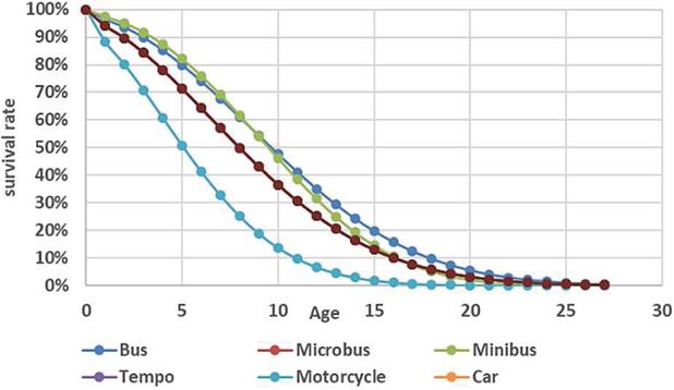
Figure 1 Survival rate of modes of passenger transport.
Since the energy demand is directly influenced by the vehicle travel demand, predicting future travel demand is vital for transport modelling. In this study, the total passenger travel demand is first projected based on the population and GDP/capita growth rate of the valley. The population residing in the city is assumed to be the active population for travel. According to CBS, 58.4% population in the valley lives in the city area. Considering the valley urbanization rate of 3.4% [15, 22], the share increases to 71% in 2017 and 79% in 2020 and is assumed to remain the same onwards. The future population is projected based on CBS and UNDESA estimates for 2020–2050 (Table 1).
The future travel demand is then estimated using Equation (2) adopted from [9] which reflects the effect of economic growth on the passenger travel demand. The estimated GDP/capita for 2017 was 2,584 USD at current prices against the national average of 877 USD in the same year [23]. Before the pandemic, the GDP growth rate was expected to grow at 6.3% per annum [24] which squeezed to 1.8% [25] during 2019–2020 due to COVID-19. However, the economic growth is estimated to rebound to 3.5% during 2020–2025, 5.3% in 2025–2030, 5.7% to 2030–2035, 6% in 2035–2040, 6.3% in 2040–4045 and 6.6% in 2040–2045 [26]. Since there is no study on the economic growth rate of Kathmandu valley, the economic growth rate of the valley is assumed the same as that of the country.
| (3) | |
Equation (3) assumes a hypothetical point to estimate income and mobility of any region by geographically decoupling such that as the slope e becomes 1, the per capita income of people will be 240,000 USD. The region-specific constraints g, h, and e for South Asian Countries are 13.2, 54.95, and 0.769, where e is the slope and f is the intercept [9]. Using this equation, the travel demand in 2017 was estimated to be 11 billion passenger-kilometer (BPKM) and the future travel demand is estimated as shown in Table 1.
Table 1 Forecasted valley population and assumed population growth in Kathmandu valley and total passenger travel demand
| In millions | 2017 | 2020 | 2025 | 2030 | 2035 | 2040 | 2045 | 2050 |
| Valley | 2.95 | 3.19 | 3.51 | 3.79 | 4.06 | 4.30 | 4.52 | 4.73 |
| population | 2017– | 2020– | 2025– | 2030– | 2035– | 2040– | 2045– | |
| 2020 | 2025 | 2030 | 2035 | 2040 | 2045 | 2050 | ||
| Valley population growth rate (%) | 2.56 | 1.92 | 1.57 | 1.37 | 1.1 | 1.0 | 0.89 | |
| Travel demand billion (PKM) | 11 | 15 | 16 | 19 | 23 | 29 | 36 | 45 |
| [15, 27]. | ||||||||
In this study, the future transport modal mix and energy mix is carried out considering the travel behaviour of consumers using the attribute travel time into the model. The travel time depends on the speed of each mode of vehicle an individual chooses. So the vehicle speed in normal traffic conditions is assumed as an input variable for the travel time estimation. Literature studies have shown that the conceptual model better represents travel behaviour. So the travel time budget (TTB) approach is incorporated into the TIMES model. For this, the travel time spent in a motorized mode is estimated using the time efficiency (inverse of travel speed, hr/pkm) factor. The time efficiency is specified in terms of time taken in an hour per vehicle kilometer traveled. This parameter is linked to travel behavior, as most passenger prefers to travel in high-speed travel mode which could be seen by the increasing number of 2-WHs (motorcycle) in the valley. The vehicle speed of each mode is given in annex A.3.
The total motorized travel time is thus estimated using equation 4 where TVi is the travel demand of mode i and vi is the speed of mode i. Thus the total motorized passenger travel time is found to be 1134 PMhs (Passenger Million hours). Given the growth rate of travel demand of 4.3% and population growth rate of 1.4% from Table 1, the per capita travel time is estimated to be 0.97 hr/capita/day in 2017 and is expected to increase to 1.09 hr/capita/day in 2050 whereas total travel time budget is expected to be 1857 PMhs in the end year. The relationship between travel time and travel demand is given by Equation (4) [12].
| (4) |
A TIMES model framework is used considering the robustness of the model in examining the attributed factors along with the time constraint. There are two input commodities, namely time input and fuel input, to produce energy service demands of all technologies. The time commodity describes the total travel time from origin to a destination, which is dependent on modal speed. Travel time is primarily affected by technology, infrastructure, congestion, accessibility. In this model, TIME input is given by TTB such that the time commodity availability is fulfilled by mining TTB. Gasoline, diesel, and LPG are imported to avail fuel to each technology. The time input is initially bounded for a reference scenario and is updated in other scenarios On the Demand side, passenger-kilometer travel demand is provided exogenously to the model. The existing technologies are vintage to their remaining life. So, to fulfill the remaining demand, new technologies like new buses and new cars evolved. The new technologies are characterized by investment cost, starting period, and efficiency.
The travel time enabled the technology to compete based on the cost of time in addition to technology cost. It thus allows the model to select the cheapest technology based on both parameters instead of selecting the cheapest yet slower mode which does not reflect the travel pattern of the users.
The model determines PKM and travel time investment subject to Equation (5):
| (5) |
Where, is the travel demand for technology t and demand d and cost is the sum of fuel, investment, fixed O&M, and cost of travel i.e
where fuel cost is a product of the price per unit of energy of fuel and the energy intensity of the technology, divided by the load factor (LF). The cost of travel is attributed as variable OM cost in Rs/pkm, depends on the speed of the vehicle given by:
where is the time cost in Rs/hr is the speed in kilometers per hour of technology t. The model is subject to two main constraints, firstly, that technologies meet the exogenously defined travel demand, given by Equation (6):
| (6) |
secondly, that the total yearly travel time of the system does not exceed the total travel time budget (TTB), given by Equation (7):
| (7) |
The model thus gives the optimal energy modal mix based on the given constraints. Future transport modal mix is then analysed under different scenarios by not only considering the transport activities but also incorporating the travel behaviour into the model.
2.1 Scenario Assumptions
The scenario analysis is carried out for five different transport scenarios to predict future modal mix and its associated energy and emissions. The major assumptions and parameters considered in each scenario are described below in Table 2:
Table 2 Scenario assumptions and parameters
| Assumptions/Parameters | ||||||
| Travel | Bounds | |||||
| Modal | Time | BRT | on | |||
| Scenarios | Mix | Fuel Mix | Constraint | Optimization | Intervention | 2 WHs |
| S1 | Fixed | Fixed | ||||
| S2 | Fixed | 50% electric | ||||
| S3 | Least cost | Optimized | ||||
| S4 | Least cost | Optimized | ||||
| S5 | Least cost | Optimized | ||||
S1: Reference Scenario
This reference scenario signifies the outcome of the TIMES model structure in business as usual. The model is first to run without any constraint and the modal mix is assumed the same during the analysis period in this scenario. The model result would thus give energy demand and emissions based on travel demand and the fuel economy of individual mode.
S2: ELE scenario (Electrification)
The market penetration of the electric vehicle is evident with the growing concern over clean transportation technology. The existing policy has set the target to substitute fuel demand by electricity by 50% by 2050. This has been incorporated in this scenario by assuming a fixed share of electric vehicles. It gives energy-saving potential in transport as a result of penetrating clean energy.
S3: No TTB scenario (No Travel Time Budget)
In this scenario, the model is run without imposing a fixed modal share, such that the model can freely choose the least cost modal mix based on technology and fuel cost. Once the old vehicles retire, the cheaper modes of transport would be chosen.
S4: TTB scenario (With Travel Time Budget)
A travel time budget (TTB) is introduced into the model based on the projected passenger-kilometer (PKM) per capita. The available time is bounded such that the modal mix would meet all travel demands within the given travel time budget. It allows faster modes of transport, particularly private vehicles, to compete with low-cost private vehicles. Individual preference for faster modes of transport is reflected in terms of cost of time. in addition, the PKM/capita which grows faster than TTB would push the model to choose faster modes of transport to meet the growing demand within a limited time. This scenario gives the least cost based on technology cost, fuel cost, and time cost. Time cost represents the comparative cost of travel in each mode, which is thus dependent on the speed of vehicles. The higher speed of vehicles reduces the cost of travel and vice-versa.
S5: TTB POL scenario (Travel Time Budget with Policy intervention)
The new public transport technology is introduced in this scenario along with the S4 scenario. To reduce the growing 2-wheelers dominance as well as represent the shift to private cars with income growth, bound on 2-wheelers is also set in this scenario. The introduction of higher speed rapid transit represents the infrastructural investment in reducing the cost of travel time. The lower cost of travel time would allow rapid transit to compete with other modes of transport.
3 Results and Discussions
3.1 Base Year Travel Demand and Energy Consumption
In 2017, travel demand was 11 billion passenger kilometers (bpkm) which increased to 15 bpkm in 2020. During the same period, the modal mix remains almost the same with 2-wheelers’ dominance over other modes. The overall passenger transport consumed 5PJ of energy which is approximately 15% of the total transport energy demand in the country in 2017 and increased to 7PJ in 2020. The energy consumption by fuel and mode in 2017 and 2020 is as shown in Figure 2. The fuel mix in 2020 shows more than 60% fuel as gasoline followed by Diesel (35%) and LPG (2%). Meanwhile, public transport (bus, microbus, minibus, 3-wheelers) consumed 30% of energy most of which is diesel and remaining by private transport (car, jeep, van, 2-wheelers) which are 95% gasoline operated.

Figure 2 Energy consumption by fuel and vehicle type in 2017 and 2020.
3.2 Scenario Results
The scenario results show the optimal modal mix in all five scenarios, energy consumption, emissions, and travel time in each scenario. The scenario analysis gives the overall transport scenario under different policy implications.
3.2.1 Modal mix
The scenario results for modal mix show the drastic modal shift with the introduction of travel time along with the fuel switching. The results illustrate the contrasting modal shift pattern as the cost of travel time is introduced as it makes the low-speed transport such as bus and minibus costlier than the comparatively higher speed vehicles such as 2-wheelers (motorcycles) and cars. Low-speed transport becomes the cheapest mode when the travel constraint is lifted. It indeed shows the effect of travel time on the modal mix and emphasizes its need to incorporate the travel behaviour during the transport modelling to represent the real scenario. It further indicates the drawback of the public transport system that the long travel time by bus makes it costlier and to promote public bus, it has to be conveniently available for the users to reach the destination with much reduced time than the existing. Since, sustainability in transport as assured by the SDGs goals, which Nepal also vowed to meet, is one of the prominent policies that promote public transport, but what is also vital in the successful implementation of the policy is how the policy would be perceived by the users at the end-use level. From this modal mix analysis, it is evident that without improving the existing system of public transport, only adding public buses would ultimately cripple the transport system as both public and private transport would increase exceedingly.
The modal mix in five different scenarios as well as vehicle stock is as shown in Figure 3. The reference scenario S1 shows the model mix without any policy intervention such that the share of each mode would remain the same. Scenario S2 represents the electrification in the existing situations which replaces 50% of public transport by electric and also introduces the modal shift from private transport to public bus. This scenario represents the policy implementation approach but it excludes the recipients’ perception on modal shift and also the mix is not optimal as the fixed share of travel demand forms the exogenous input to the model. However, the last three scenario results give the least cost modal mix: S3 without travel bound to choose the public bus, S4 with travel bound choose 2-wheelers and S5 gives a mix of the public bus, 2-wheelers, cars, and new rapid transit modes. In S5 scenarios, the share of private vehicles (car/jeep/van) would increase to 63% by 2030 and then be reduced to 20% by 2050. Meanwhile, motorcycle share decreases to 25% by 2030 and 10% by 2050 from the current 35% share. Introduction of bus rapid transit (BRT) from 2030 replaces other modes contributing 70% share by 2050 as shown in Figure 3.
As seen from the modal mix scenario, the 2-wheelers are the only cheap modes of transport for the individual, considering their time available for the travel, with small numbers of cars competing to meet the demand by 2050 (Figure 3d). It is thus evident to promote robust public transport such as BRT (Bus Rapid Transit) which can compete with 2-wheelers and cars and also meets the travel demand. The bus rapid transit which has a higher occupancy rate lowers its cost per PKM and its comparatively higher speed than public bus even lowers its overall cost to compete with 2 wheelers and cars, represented by the S5 scenario (Figure 3e). The S5 scenario shows the mix of all modes of transport representing the realistic future transport modes and also towards sustainability.
The vehicle stock on the other hand (Figure 3f)) shows the exceedingly high number of vehicles in the S1 scenario as the current situation continues adding to the current traffic problems. Meanwhile, it is possible to reduce the exceeding traffic by shifting to public transport which would significantly reduce the vehicle traffic compared to the S1 scenario by considering only the fuel switch as in the S2 scenario. But this scenario would succeed only if there is a linear shift from the user’s side as well. Certainly, the shift to public transport would considerably reduce traffic volume as is shown by the S3 scenario and would be opposite when there are only private vehicles. The optimal modal mix in the S5 scenario shows the potential reduction in vehicle traffic as well as promoting mass transport and public vehicles.
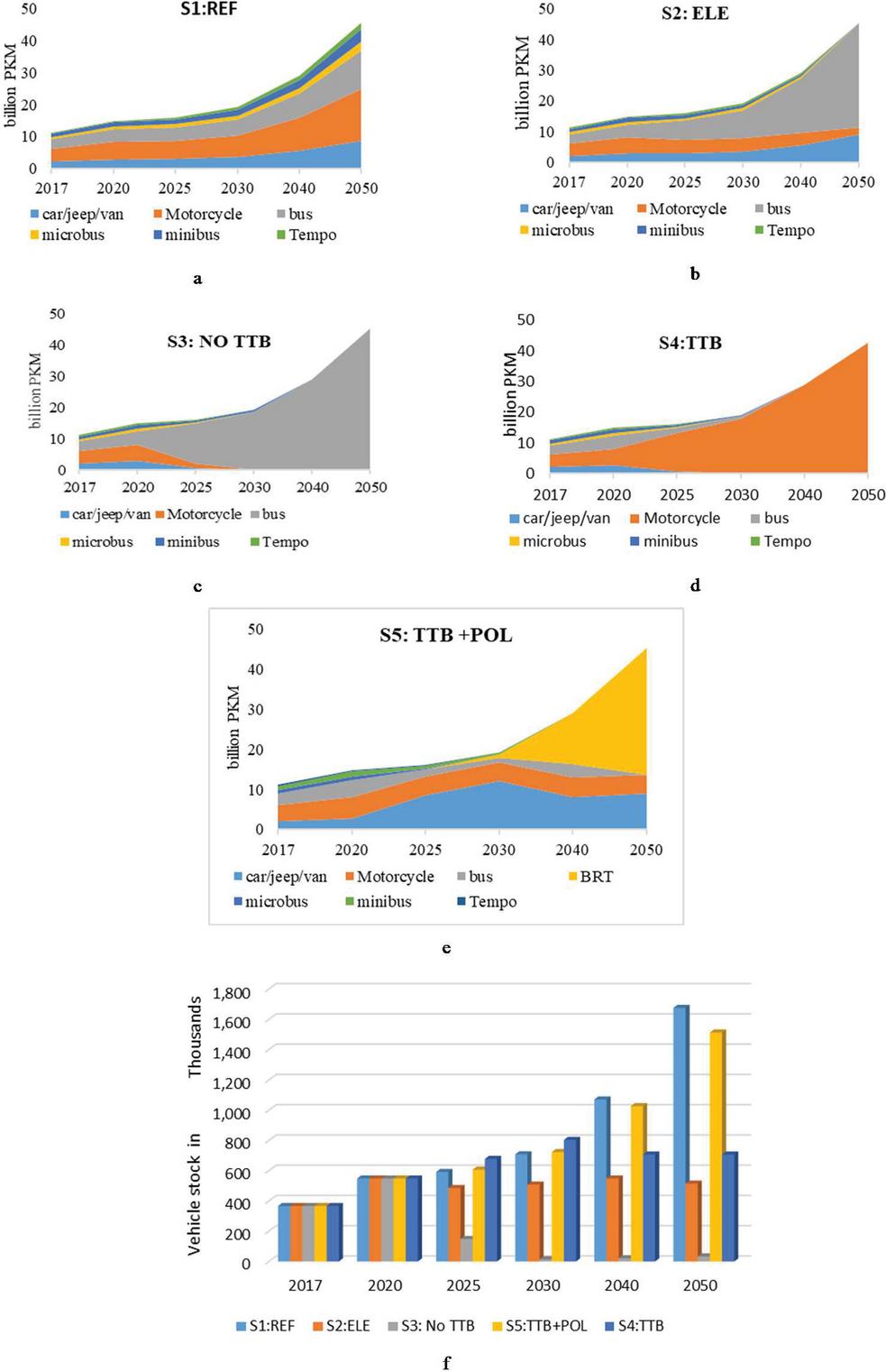
Figure 3 Modal mix and vehicle stock in different scenarios.
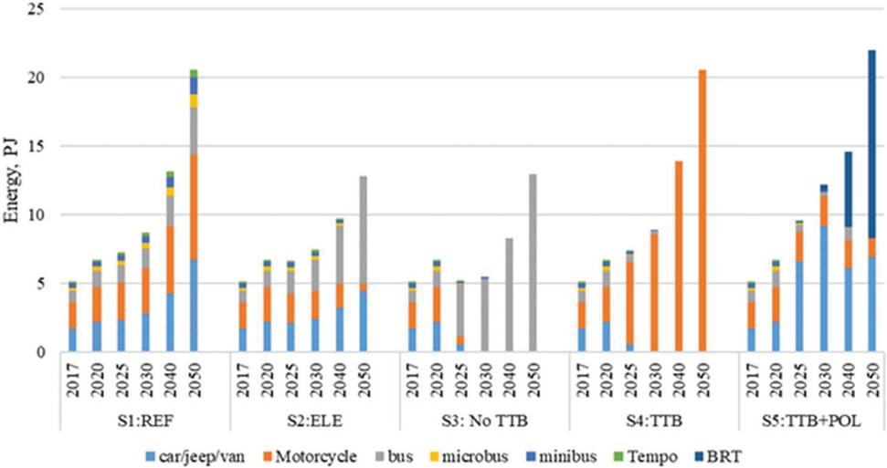
Figure 4 Transport energy demand in different scenarios.
3.2.2 Energy and emissions
As the energy and emissions are influenced by modal mix, energy demand and GHG emissions in different scenarios are shown in Figure 4. It was found that energy demand would increase from 9 PJ in 2030 to 21 PJ in 2050 in the reference scenario which could be reduced by almost 38% with the introduction of more efficient electric vehicles in the S2 (electrification) scenario. The optimal modal mix shows different results with high energy demand in the S5 scenario where there is a mix of bus, car, 2-wheelers, and electric rapid transit vehicles. The S3 scenario shows lower growth in energy demand to 13 PJ by 2050 due to the replacement of all energy-intensive modes by the energy-efficient public bus but it only increases dependency on petroleum products as 100% of it would be petroleum-based. Meanwhile, the S4 scenario reveals that shifting to 2-wheelers while meeting the travel time budget would increase energy demand at the rate of 4% per annum, and but there would be a huge stock of 2-wheelers which is beyond sustainability. The energy demand in the S4 scenario is slightly higher than all scenarios as there is a mix of both energy-intensive private vehicles as well as energy-efficient public vehicles increasing at the rate of 4.5% per annum to 22PJ by 2050. The fuel mix in this scenario shows 64% electricity followed by 31% diesel and 5% gasoline in 2050. there would be 63% energy demand from newly penetrated BRT and 31% from private/car/jeep/van, and 6% from the motorcycle. To fulfil this electricity demand in passenger transport, it requires an installed capacity of 855 MW of electricity by 2050.
The cumulative COe emissions between 2017–2050 in S1 and S2 scenarios are 6,389 kt and 3,788 kt, a significant reduction of 41% in the S2 scenario. The cumulative emission shows that S3 is more environmentally friendly with 4,476 kt emissions during 2017–2050. S4 and S5 scenarios have cumulative emissions of 6,498 kt and 4,992 kt respectively during the same period.
3.2.3 Travel time budget
The exceedingly different time taken in each scenario to meet the same travel demand (pkm) is as shown in Figure 5. Due to this difference in time, the model chooses different modes of transport in each scenario. Since there is no limit of time on the S1, S2, and S3 scenarios, it can be seen that the total travel time would increase approximately to 4000 Mhs, 5000 Mhs, and 5700Mhs by 2050 respectively, whereas the available time remains at 1900 Mhs in 2050. It implies that people need to spend more time on travel than they have to due to lower vehicle speed and increasing vehicle traffic which also add up to the already higher travel time. The growing number of 2-wheelers lately is attributed to this fact and as is expected to grow in the future as well as, shown in the S4 scenario, unless intervened with rapid transit modes (S5 scenario). In contrast, even though 2-wheelers are chosen as the optimal modes in the S4 scenario, they cannot fulfill all the travel demand within the time constraint, approx. 6% remains unfulfilled in 2050, as it saturates and there are no other faster modes to switch to.
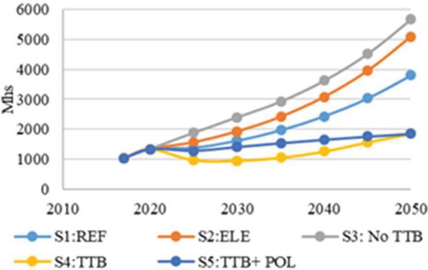
Figure 5 Total travel time in different scenarios.
3.3 Discussions
The scenario results show potential future modal mix under different scenarios and the consequent impact on energy, emissions, and vehicle stocks. Most of the transport scenario analysis does not incorporate the travel behaviour leading to the modal shift and fuel switching based only on the replacement policy of the government, as depicted in scenarios 1 and 2. It is expected that the private vehicles will be replaced by electric public buses, but, the existing scenario shows that 2-wheelers annual registration is increasing at the rate of 10% per annum and more than 90% of passenger vehicles registration are private. The underlying reasons are availability and accessibility. It takes double the time to reach the same destination by private cars than public buses during the peak hour and the accessibility to the public buses is also poor in the valley [28]. Since 2-wheelers are much cheaper (capital cost), faster, and are accessible at the doorstep, it is popular and preferred at large in developing economies, which has exceedingly increased traffic making it difficult to travel in peak hours. A similar situation would continue in the future as shown by scenario S4 unless intervened with strong policy measures which address the underlying reasons. This can be addressed by increasing the speed of public vehicles by introducing rapid transit as shown by the S5 scenario. It highlights that even though BRT seems to be a costly mode, the higher speed overcomes its capital cost making it the least cost mode which can compete with cars and 2-wheelers. This scenario seems more appealing and realistic not only from an energy and emissions viewpoint but also from the reduced vehicle traffic as vehicle stock reduces by more than 50% than the reference scenario. It even emphasizes the potential area of investment to promote public transport as a feasible, accessible, and reliable option in the future.
4 Conclusion
The analysis shows the trade-off between the speed of the vehicle, available travel time, and sustainable transport. The high cost of technology intervention to meet the growing travel demand within the specified time requires huge infrastructural investment. Financing the new technology, however, could be another setback in developing countries like Nepal where the infrastructural change hardly occurs over a decade. But considering the existing policies to move towards the path of sustainable transport such as achieving the sustainable goals by 2030, net-zero emissions by 2050, and reduction of GHG emissions and energy consumption from the transport sector as per Nepal’s second NDC (Nationally Determined Contribution), it is imperative to successfully implement the policies not by merely imposing the new policies but investing on public transport sector which could reflect the user’s travel behaviour as well. In the case of Kathmandu valley, the result suggests that the bus rapid transit, which can be readily implemented in the existing infrastructure could be the potential mode that can compete with private modes as well as promote sustainability.
This paper highlights the drawbacks of existing public transport and emphasizes investing in the potential area for improving public transport. The study also points the significance of incorporating travel behaviour in transport modelling which affects the overall transport modal mix and consequently its energy demand and emissions. It is one of the crucial parameters yet often ignored during transport planning. The study is limited to passenger transport at the city level. The study can be further carried out by linking the mode choice with the transport network to provide transportation planners with robust policy implications. The approach presented here is based on the case study of the densely populated capital city of Nepal, where 2-wheelers dominate the passenger transport and public network access is limited. The model used could be applied in other developing countries as well.
Annex
A.1 Fuel economy and fuel share of each mode
| Fuel Economy km/lt | Fuel Share | |||||
| Diesel | Gasoline | LPG | Diesel | Gasoline | LPG | |
| Bus | 3.60 | 100% | 0% | 0% | ||
| Mini Bus | 5.40 | 100% | 0% | 0% | ||
| Microbus | 6.20 | 9.27 | 9.27 | 100% | 0% | 0% |
| Tempo | 7.8 | 0% | 0% | 100% | ||
| Motorcycle | 54.00 | 0% | 100% | 0% | ||
| Car | 18.87 | 18.59 | 6% | 94% | 0% | |
| Jeep | 14.71 | 14.43 | 27% | 73% | 0% | |
| Van | 15.63 | 16.47 | 11% | 89% | 0% | |
| CEN, 219. “Baseline Study on Fuel Economy of Light Duty Vehicles (LDV) in Nepal,” Clean Energy Nepal, Kathmandu, Nepal. | ||||||
A.2 Failure rate and service life of each mode
| Parameters | Bus/Minibus | Motorbike | LDVs (Car/Jeep/Van) |
| b | 2.29 | 1.99 | 2.03 |
| T (years) | 14 | 8.5 | 12 |
| Bajracharya and N. Bhattarai, 2016. “Road Transportation Energy Demand and Environmental Emission: A Case of Kathmandu Valley,” Hydro Nepal: Journal of Water, Energy and Environment, vol. 18, pp. 30–40. | |||
A.3 Vehicle speed, time efficiency, and occupancy of each mode
| Investment | Fixed O&M | |||
| Cost | Cost | |||
| Description | Life | bRs/mpkm | bRs/mpkm | km/hr |
| Car-Gasoline | 12 | 0.008100 | 0.000203 | 12 |
| Jeep-Gasoline | 12 | 0.009703 | 0.000243 | 12 |
| Van-Gasoline | 12 | 0.005416 | 0.000135 | 12 |
| 2-Wheelers (motorcycle) – Gasoline | 12 | 0.002148 | 0.000054 | 23 |
| Car-Diesel | 12 | 0.008100 | 0.000203 | 12 |
| Bus-Diesel | 20 | 0.000292 | 0.000007 | 8 |
| Jeep-Diesel | 12 | 0.009703 | 0.000243 | 12 |
| Microbus Diesel | 12 | 0.000764 | 0.000019 | 8 |
| Minibus-Diesel | 20 | 0.000367 | 0.000009 | 8 |
| Van Diesel | 12 | 0.005416 | 0.000135 | 12 |
| 3-Wheelers (Tempo)-LPG | 12 | 0.004557 | 0.000114 | 5 |
| Bus-Electric | 20 | 0.000854 | 0.000021 | 8 |
| Car-Electric | 12 | 0.015153 | 0.000379 | 12 |
| 2-Wheelers (motorcycle) – Electric | 12 | 0.009376 | 0.000234 | 23 |
| BRT-Electric | 20 | 0.011232 | 0.000281 | 35 |
|
Annual_FTS_pdf.pdf (customs.gov.np) dotm.gov.np Shrestha, S.R., Oanh, N.T.K., Xu, Q., Rupakheti, M., Lawrence, M.G., 2013. Analysis of the vehicle fleet in the Kathmandu Valley for estimation of environment and climate co-benefits of technology intrusions. Atmospheric environment 81, 579–590. |
||||
References
[1] EIA. 2019. “International Energy Outlook 2019”, U.S. Energy Information Administration.
[2] GFEI. 2019. “Global Fuel Economy Initiative Update,” Global Fuel Economy Initiative Global Fuel Economy Initiative.
[3] S. Gota, 2018. “The road towards low carbon mobility,” ed 21 rue du Faubourg Saint-Antoine, 75011 Paris: Climate Chance.
[4] W.-S. Ng, 2018. “Urban Transportation Mode Choice and Carbon Emissions in Southeast Asia,” Transportation Research Record: Journal of the Transportation Research Board, vol. 2672, pp. 54–67.
[5] V. A. Tuan, 2015. “Mode Choice Behaviour and Modal Shift to Public Transport in Developing Countries – the Case of Hanoi City,” Journal of the Eastern Asia Society for Transportation Studies, vol. 11.
[6] G. Venturini, J. Tattini, E. Mulholland, and B. Ó. Gallachóir, 2018. “Improvements in the representation of behavior in integrated energy and transport models,” International Journal of Sustainable Transportation, vol. 13, pp. 294–313.
[7] R. Gerboni, D. Grosso, A. Carpignano, and B. Dalla Chiara, 2017 . “Linking energy and transport models to support policy making,” Energy Policy, vol. 111, pp. 336–345.
[8] J. Tattini, K. Ramea, M. Gargiulo, C. Yang, E. Mulholland, S. Yeh, et al., 2018. “Improving the representation of modal choice into bottom-up optimization energy system models – The MoCho-TIMES model,” Applied Energy, vol. 212, pp. 265–282.
[9] A. Schafer and D. G. Victor, 2000. “The future mobility of world population 2000,” Transportation Research Part A, vol. 34, pp. 171–204.
[10] M. Salonen and T. Toivonen, 2013. “Modelling travel time in urban networks: comparable measures for private car and public transport,” Journal of Transport Geography, vol. 31, pp. 143–153.
[11] S. Pye and H. Daly, 2015. “Modelling sustainable urban travel in a whole systems energy model,” Applied Energy, vol. 159, pp. 97–107.
[12] H. E. Daly, K. Ramea, A. Chiodi, S. Yeh, M. Gargiulo, and B. Ó. Gallachóir, 2014. “Incorporating travel behaviour and travel time into TIMES energy system models,” Applied Energy, vol. 135, pp. 429–439.
[13] DOTM. 2019. Department of Transport Management, Ministry of Physical Infrastructure and Transport, Government of Nepal. Available: dotm.gov.np
[14] S. Malla, 2014. “Assessment of mobility and its impact on energy use and air pollution in Nepal,” Energy, vol. 69, pp. 485–496.
[15] CBS, 2011. “Nepal Living Standard Survey 2010/11, Statistical Report, Volume One,” Central Bureau of Statistics, National Planning Commission Secretariat, Government of Nepal, Central Bureau of Statistics, National Planning Commission Secretariat, Government of Nepal, Kathmandu, Nepal.
[16] NRB, 20121. Nepal Rastra Bank, “The Share of Kathmandu Valley in the National Economy,” Kathmandu, Nepal.
[17] NOC, 2020. Nepal Oil Corporation Limited. Import and Sales. Available: http://noc.org.np/import
[18] T. Wulf, P. Meißner, and S. Stubner, 2010. “ Scenario-based Approach to Strategic Planning – Integrating Planning and Process Perspective of Strategy,” Working Paper.
[19] A. Prajapati, T. R. Bajracharya, and N. Bhattarai, 2017. “Driving Factors of Energy Consumption in Transport Sector,” in IOE Graduate Conference.
[20] S. Baidya and J. Borken-Kleefeld, 2009. “Atmospheric emissions from road transportation in India,” Energy Policy, vol. 37, pp. 3812–3822.
[21] I. Bajracharya and N. Bhattarai, 2016. “Road Transportation Energy Demand and Environmental Emission: A Case of Kathmandu Valley,” Hydro Nepal: Journal of Water, Energy and Environment, vol. 18, pp. 30–40.
[22] CBS, 2001. “Population Monograph of Nepal,” Central Bureau of Statistics, Central Bureau of Statistics, Kathmandu, Nepal.
[23] MoF, 2020. “Economic Survey 2019–2020,” Ministry of Finance, Government of Nepal, Kathmandu, Nepal.
[24] NPC, 2019. “15th approach paper,” National Planning Commission, Kathmandu, Nepal.
[25] World Bank. 2020. Nepal Development Update. Available: https://www.worldbank.org/en/country/nepal/publication/nepaldevelopmentupdate
[26] WECS, 2021. “Energy Consumption and Supply Situation of Federal System of Nepal (Province No. 1 and Province No. 2),” Water and Energy Commission Secretariat, Government of Nepal, Kathmandu, Nepal.
[27] UNDESA, 2019. “World Population Prospects 2019,” United Nations Department of Economic and Social Affairs Population Dynamics.
[28] A. Prajapati, N. Bhattarai, and T. R. Bajracharya, 2020. “Spatio-Temporal Analysis Of Public Transportation System Using Static Transit Accessibility Methodological Framework,” International Journal of Scientific & Technology Research, vol. 9.
Biographies

Anita Prajapati is a Ph.D. scholar in the Institute of Engineering (IOE), Tribhuvan University (TU), Nepal under the scholarship of a Norwegian Program EnPe (Energy and Petroleum). She received her BE in Mechanical Engineering and M.Sc. in Renewable Energy Engineering from the IOE. She is presently working as an assistant professor in the Department of Mechanical and Aeropsace Engineering in the Pulchowk Campus, IOE, TU having teaching experience since 2018. She is also working as Research Associate in Centre for Energy Studies, IOE, TU. She has presented papers at national conferences. Her area of interest includes energy modeling and systems planning analysis.
Nawraj Bhattarai is the former Head of Department of Mechanical and Aeropsace Engineering Pulchowk Campus, Institute of Engineering, Tribhuvan University, Nepal. His field of specialization is energy planning, renewable energy Engineering and energy policy. He did his Doctoral Degree in Mechanical Engineering from Vienna University of Technology, Vienna, Austria in the year of 2015. He has published many research papers in National and International journals.
Tri Ratna Bajracharya is the former Dean of Institute of Engineering, Tribhuvan University, Nepal. He is a permanent full Professor of Department of Mechanical and Aeropsace Engineering, Pulchowk Campus, Institute of Engineering, Tribhuvan University. His field of specialization is energy systems; especially renewable energy technology. He was the Director for Centre for Energy Studies (CES) for more than 5 years. He did his Doctoral Degree in Engineering from Tribhuvan University in year 2007 in Hydropower technology. Prof. Bajracharya is well-known expert in the field of energy and climate change and has published many research papers in International Journals. He has served as the Chief Editor of Journal of the Institute of Engineering, ISSN 1810-3383.
Strategic Planning for Energy and the Environment, Vol. 40_3, 231–254.
doi: 10.13052/spee1048-4236.4032
© 2021 River Publishers