Short Term Solar Irradiation Prediction Framework Based on EEMD-GA-LSTM Method
Anuj Gupta1,*, Kapil Gupta1 and Sumit Saroha2
1Maharishi Markandeshwar (Deemed to be University), Mullana-Ambala, India
2Guru Jambheshwar University of science and Technology, Hisar, India
E-mail: annu11gupta@gmail.com
*Corresponding Author
Received 09 November 2021; Accepted 23 March 2022; Publication 28 April 2022
Abstract
Accurate short term solar irradiation forecasting is necessary for smart grid stability and to manage bilateral contract negotiations between suppliers and customers. Traditional machine learning methods are unable to acquire and rectify nonlinear characteristics from solar dataset, which not only complicates model construction but also affect prediction accuracy. To address these issues, a deep learning based architecture with predictive analysis strategy is developed in this manuscript. In the first stage, the original solar irradiation sequences are divided into many intrinsic mode functions to generate a prospective feature set using a sophisticated signal decomposition technique. After that, an iteration method is used to generate a prospective range of frequency related to deep learning model. This method is created by linked algorithm using the GA and deep learning network. The findings by the proposed model employing sequences obtained by the preprocessing methodology considerable improve prediction accuracy as comparison to conventional models. In contrast, when confronted with a high resolution dataset derived from big data set, the chosen dataset may not only conduct a huge data reduction, but also enhances forecasting accuracy up to 22.74 percent over a variety of evaluation metrics. As a result, the proposed method might be used to predict short-term solar irradiation with greater accuracy using a solar dataset.
Keywords: Solar irradiation, EEMD, genetic algorithm, LSTM, evaluation metrics.
1 Introduction
Because of the greenhouse effect, pollution and the depletion of natural resources it is now more vital than ever to use renewable energy sources (RES) that do not pollute the environment and free to use to create electricity. Among RES, solar energy is one of the most popular energy sources for generating electricity with zero carbon emission and its market is growing significantly due to its long-term viability and support [1]. Almost every year, the earth’s surface receives around 1.5 10 KWh/area of solar energy which is nearly ten times the current global usage. Among all Asian countries, China receives the highest annual average daily global solar radiation (20.2 MJ/(m.d)) while India receive just (18 MJ/(m.d)). The renewable energy sector in India, as an example of emerging countries, has grown at an exponential rate during the last two decades. India has even established a special ministry for RES; Ministry of New and Renewable Energy (MNRE), with a goal of generating 175 GW of energy from RES by the end of 2022; with 100 GW from solar alone [2, 3]. Furthermore, according to several studies, the power grid will be completely functioning on the renewable energy source (RES) by the end of 2050 [4]. But, due to the variability in weather condition; the intensity of solar GHI is unstable which directly affect the output of photovoltaic power plant [5]. Result in poor reliability of photovoltaic power plant. So, a number of forecasted models are developed in the literature to increase the solar GHI forecasting accuracy [6]. The solar irradiance forecasting technologies are classified into four categories: (1) Physical method (2) Machine learning method (3) statistical method (4) Hybrid methods [7–11]. The physical models uses meteorological and geographical parameters as an input to forecasting the model and set up a mathematical relation between meteorological data and forecasted GHI. Due to its complexity, less precision and high computational cost, these models are not popular among researchers [12–14]. The statistical methods such as Gaussian Progress Regression (GPR) [15, 16] autoregressive integrated moving average (ARIMA) [17] improve forecasting accuracy and set up a mathematical relation between meteorological variables and GHI but the poor correlation among input data and solar GHI leads to weak performance of these models performance. The machine learning models such as artificial neural network (ANN) [18], Elman neural network (ELMAN) [19] and support vector machine (SVM) [20] have a capability to learn itself and reduce the gap between forecasted and measured data Nevertheless, due to uncertain behavior of GHI, single machine learning models stuck in local minima and do not perform efficiently [21]. Therefore, hybrid models are discussed in literature to overcome these issues. The data decomposition based technique and machine learning model is one of the mostly used hybrid models. Several decomposition techniques such as wavelet Transform (WT), empirical Mode Decomposition (EMD), variational Mode Decomposition (VMD) etc are discussed in previous studies. The author [22] uses the EMD decomposition technique to decompose the input data and auto regressive (AR); ANN model are used to estimate the GHI. The experimental result shows that the hybrid model achieves better result as compared to standalone AR and ANN models.
In addition, deep learning emerged as a powerful technique to forecast the solar GHI and its performance is much better than conventional models in all aspects. In literature, a number of researchers suggested deep learning technique with preprocessing strategy to enhance the accuracy of forecasting model. The author of [26] uses long Short Term Memory (LSTM) network to forecast the GHI; where weather data is used as an input to the LSTM network. The study proves the efficiency of LSTM network over BPNN, linear regression in terms of RMSE. A hybrid model of LSTM and gradient boosting algorithm are implemented by the author of [27] to prevent the situation of over fitting and compared with naïve predictor and SVM model. The performance of ensemble approach shows that proposed model significantly improves the result in terms of RMSE. Similarly [28] developed a hybrid approach to forecast the solar irradiance using a combination of Convolution Neural Network (CNN) and LSTM. The historical properties of the input data are acquired by using an LSTM network and the geographical data is obtained using CNN. In addition to deep learning network, various data decomposition techniques used as a preprocessing strategy to decompose the irradiance data, clean up and define the input data according to the specifications. The SOM, WT, EMD, EEMD, normalization, kalman filter are often used in solar irradiance forecasting. It is confirmed in a number of prior studies that WT-based models obtained satisfactory results due to their outstanding localization properties in both the temporal and sensitive attribute. However, it’s not clear how to pick the right wavelet function for a set of data [34]. Same humiliation is occurs, when using VMD preprocessing approach, where the number of modes is an a priori value that must be specified at the start, but has a major impact on the decomposition results [35]. Given that by adding intrinsic mode functions, the EEMD technique displays its astonishing superiority in automatically responding to any irregular time-series [36]; when confronted with such a challenge, it may be the best alternative. Prasad et al. [37] developed an EEMD-RF model for multi step ahead solar GHI forecasting. The author adds the results of all sub-predictions from LSTM model, then rectifying the summation using ant colony optimization technique. Qin et al. [38] uses fuzzy classification technique with EEMD-LSTM model. In this study, EEMD divide the incoming data into many IMFs, fuzzy classification technique categorizes the IMFs into a number of groups and used LSTM predictor for each group and summing all predictions to obtained final result. These studies have established a good base for applications that combine EEMD and LSTM learning models.
However, the problem is that it is useless unless the number of sub-series is determined in advance using EEMD-based models. Because as the solar dataset’s temporal resolution improves and the recording period lengthens, the dataset scale widens, resulting in increased non-linearity and non-stability in the solar time series. The number of IMFs will increase dramatically as a result of using the EEMD approach on such a massively dataset. As a result, at least two barrier processes keep following the routines described in the preceding literatures [36–38]. Firstly, more IMF components would result in more untrained data in which raising the overall training cost. Secondly, if machine learning model employ to predict the IMF components and forecasting error of each component add up to the final error in which affect the prediction accuracy of model.
Therefore, with an aim to address this problem and increase to prediction accuracy; this paper proposes a new framework that combines EEMD: a signal decomposition technique, Genetic Programming: a feature selection technique and LSTM: deep learning model. Unlike some prior work in this field [37, 38], all decomposed component from EEMD method are no longer used for solar irradiation construction but to provide a prospective feature set for LSTM model to learn from. Secondly, Genetic Algorithm decreases the size of the projected feature set collection and changes it into a subset with more useful data.
Taking into account all of the preceding processes, the following are the primary contributions of this work:
• To deal with the increasing scale of datasets, a unique architecture of ensemble learning system incorporating EEMD, GA, and LSTM for solar irradiation forecasting is presented. Rather than following the “decomposition—prediction—reconstruction” design used in previous investigations [36, 37], the suggested framework attempt to deliver a more compact and useful set of features out of a total prospective IMFs obtained by EEMD technique.
• In this framework three year data of Delhi location collected from NSRDB (National Solar Radiation Database). Two year data used for training and one year data used for testing on seasonal basis. The testing data is dividing into seasons: winter, spring, summer, monsoon and autumn as given in Delhi Tourism website [39].
• A detailed comparative evaluation of the results is undertaken in this work from a progressive multi-level.
Unlike previous studies [36, 37], where comparisons with other models are made all at once, this study focused on progressing features. First, a comparison between the present framework and non-EEMD machine learning models is made. Then it moves on to a comparison of models that use the EEMD approach. In the proposed models we check the effectiveness of EEMD decomposition, genetic algorithm feature selection technique and long short term memory neural network model.
The remaining sections of this paper are organized as follows: Section 2 will begin with a theoretical background of EEMD and data driven model. The mechanism for solar irradiation forecasting framework will be explained in Section 3. Section 4 will look at the suggested model’s outcome as well as comparisons to other models.. Section 5 concludes the present work.
2 Theoretical Background of EEMD and Data Driven Model
2.1 Ensemble Empirical Mode Decomposition
Huang et al. [40] introduced a decomposition technique based on Hilbert Huang Transform in 1998 called Empirical Mode Decomposition (EMD). The technique is used by various researchers due to following advantage: 1. it can handle irregular and unstable information 2. Unlike wavelet transform or Fourier transform which require a pre-specified foundation, HHT is entirely approach by introducing intrinsic mode functions (IMFs). However, a few of these IMF include fluctuations of wildly varying magnitude and this phenomenon is known as “mode mixing.” These fluctuations cause the IMFs to lose their scientific significance and also reduce the physical significance of EMD algorithm. In order to address these issue, an improved version of EMD called EEMD has been introduced in year 2009 [41].
The procedure of EEMD is given as [41]:
1. Creating a new signal by combining a Gaussian based stochastic signal with the desired sequence [41]
2. Using the EMD approach, decompose . Obtain the IMFs and residue [41]
3. Carry on with the previous steps. The input sequence is subjected to unique white noise each time [41]
4. When the Gaussian white noise average value is zero, the final decompositions IMFj(t) will be the grand average of all matching IMFs [41]
| (1) | ||
| (2) | ||
| (3) | ||
| (4) |
2.2 Long Short Term Memory Neural Network (LSTM)
J.J. Hopfield developed a recurrent neural network (RNN) in 1982. In this network, the RNN is related to the input via feedback acting like a dynamic memory. For short term forecasting this network worked best, but for long term forecasting it becomes unstable. This inconsistency caused by gradient boosting i.e. substantial changes in training weights in a short period of time. This problem is solved by LSTM to permit using of memory cells in a hidden layer. These memory cells are utilized to store information in an appropriate manner. The basic configuration of LSTM network is shown in Figure 1. Each memory cell having a forget gate , input gate and output gate to accept or reject any information. For a forward movement function, the previous cell state discarded by the LSTM network [42]
| (5) |

Figure 1 Basic configuration of LSTM network.
The LSTM network use the equation below to determine whether data information should be discarded or maintained [42]
| (6) | ||
| (7) | ||
| (8) |
Now the memory cell output represented as [42]:
| (9) | ||
| (10) |
3 Structure of the Proposed EEMD-GA-LSTM Framework
The goal of this project is to increase the accuracy of Solar GHI forecasting by employing an EEMD-based LSTM network with binary coded genetic algorithm. Figure 2 show the schematic diagram of the developed model and its steps is discussed below:
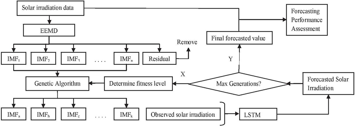
Figure 2 Schematic diagram of the proposed model.
3.1 Data Description and Quality Assurance
The dataset of Indian location is used in the study to forecast solar GHI because of the substantial improvement in the infrastructure of renewable sector in India. For this, three year hourly data is used for training, validation and testing purpose. Table 1 provides a geographical coordinates, climatic condition and clear sky hour’s details of the selected location.
Table 1 Geographical details of Delhi Location
| Rainfall | Clear-Sky | Altitude | |||||
| Location | (mm) | Hours | Climate | (m) | Longitude | Latitude | Region |
| Delhi | 714 | 2809 | Cwa, Bsh | 225 | 77.1025E | 28.7041N | North |
| Cwa Humid Subtropical; Bsh Hot semi-arid. | |||||||
The input data has great impact on the model performance. Primarily, the collected data is available in its raw form which is random and non-linear in nature and has a great influence on the effectiveness of the model. Due to the weak pyranometer reaction, there is a chance of finding incomplete and negative data recording [28]. Therefore these data recordings must be deleting before feeding to forecasting model. To enhance the quality of input data, this paper calculates normalized value of data in which convert the data in stationary form. The normalization is calculated as follows [14]
| (11) |
represent the standardized value, is the value to be normalized, is the maximum value in all the values for related variables and is the minimum value.
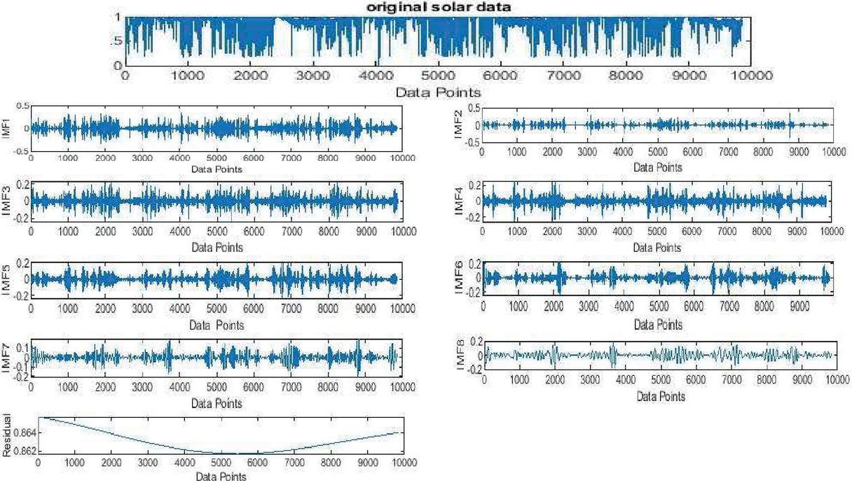
Figure 3 EEMD Decomposition results.
3.2 Binary Coded Genetic Algorithm
In feature extraction architecture and computational intelligence research, the wrapper is crucial. This study adopted the binary coded based GA to discover the best IMF as the feature set for training of LSTM in order to enhance the current solar irradiation predictor performance.
3.2.1 Binary coding
All eight IMFs are arranged from IMF1 to IMF8 to transfer in a small set of 1 and 0 (binary list) as shown in Figure 4. Combining these two lists via elemental multiplication yields the final selected list of IMFs. This allows us to decide whether IMF should be discarded or retained. The element under the binary list relevant index is set to 1 if an IMF is required; otherwise, it is set to 0.
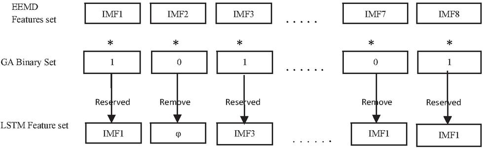
Figure 4 Genetic Feature selection in binary coding.
3.2.2 Initial trails
For searching algorithms like GA, a proper initial condition is necessary because it can not only supply viable trails from the start but also disperse the searching spots globally. On the basis of these two considerations, the original population in this study is made up of binary sets as follows:
I. All of the elements have been set to be one.
II. The value of all items has been set to zero.
III. The first half of the elements has a value of one, while the second half has a value of zero.
IV. The first halves of the components are assumed to be 0, while the latter half is assigned to 1.
V. The items with the highest Correlation coefficient with the raw sequences are given a value of one while the others are given a value of zero.
VI. The elements having the highest Pearson correlation with the raw sequence have their associated IMF’s set to zero while the others are set to one
The Pearson correlation for a set of objective variables (P, Q) is given as [38]
| (12) |
Where P denotes the unprocessed value and Q denotes the intrinsic mode functions; and indicate the estimation and random deviation respectively.
3.2.3 Fitness
The best solution of this task is given as [38]
| (13) |
Where represent the mean absolute error among the forecasted and measured sequence on given data utilizing as the binary list for extracting features.
3.2.4 Evolutionary procedure
Selection, crossover, and mutation all are parts of GA evolutionary process. These parts provide an overview of the main process.
Selection
There are two prerequisites to the selecting method. First, a generation greatest individual will sustain themselves and bypass this filter. Furthermore, individuals with a higher level of fitness will have a greater chance of joining the next generation; Probability is calculated by the below equation [38]
| (14) |
Where denotes the th individual in the th generation, and m represent the population size.
Crossover
Each DNA candidate will have the opportunity to recombine with another person from the same generation (i.e. crossover rate). The DNA information from both parent sets will be inherited by the young individual. The participants and cross-points are picked at random for every cycle of crossover, as inspired by “the law of independent assortment” [41].
Mutation
A mutation mechanism is implemented after the crossover to minimize the pre-mature issue and to further broaden the seeking area. Should one of the DNA elements is changed, it goes from 0 to 1 or 1 to 0 but this operation does not have to be repeated on all members of DNA collections every moment. As this may produce divergence issues and raise computation costs.
3.3 Performance criteria
In this study, two year data set is utilized as the learning unit, whereas one year data is used as the testing dataset. To obtain the performance of developed model, the testing data set is dividing into five seasons: winter, spring, summer, monsoon and autumn. Assume is the solar irradiance time history and is the forecasted solar irradiance time series, used to calculating the performance of proposed model [2, 3].
Mean Absolute Error (MAE): This metric provides a difference between two set of data using Equation (15) [2]
| (15) |
Mean Absolute Percentage Error (MAPE): It provides uniform forecasting error in percentage using Equation (16) [2]
| (16) |
Root Mean Square Error (RMSE): It is a statistic for assessing the largest expected error in the forecasted data.
Using Equation (17) [2]
| (17) |
Where n represent total number of points.
4 Result Analyses
This study uses a combination of EEMD-GA-LSTM to improve forecasting accuracy. The developed model performance is compared with standalone models: Naïve Predictor, Gate Recurrent Unit (GRU), Recurrent Neural Network (RNN), Extreme Learning Machine (ELM), Back Propagation Neural Network (BPNN) and other EEMD based models. All experiments are performed using MATLAB 2019a and numerous models scenarios are analyzed. Firstly, the results of the selected features from the GA are discussed. Secondly the proposed model performance is compared with naïve predictor, standalone GRU, BPNN, ELM and RNN model. Next, EEMD method is apply to the all above mentioned standalone models and finally, evaluation of the selected features is study.
4.1 Result of Feature Selection
In this study, the range of GA is set to 30 to balance the exploring ability and model cost. The synchronization lines of the mean and the optimum fitness among community are displayed in Figure 5.
As can seen in Figure 5, the average fitness increase steadily over the first 15 iterations and then gradually stabilized after that despite minor oscillations. The best fitness grew slightly over the first five generations but remains practically unchanged after that indicates the possible selected features are discovered early. Because the average activities has not yet convert to the fitness values, an earlier halt is possible because the modification in fitness value is expected to be flat at this time.
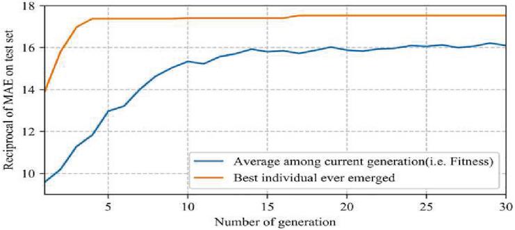
Figure 5 Generational changes in average and optimum fitness.
4.2 Analysis and Assessment by Comparison
In this portion, the discussion would be split into two sections: For the comparison study in the first half, various mainstream models will be considered. In the second half, on the basis of selected features evaluation, the result obtained by the proposed model is compared to the standalone LSTM model and the EEMD-LSTM model which consist all prospective features.
Case 1: Comparative research with standalone models The goal of this scenario is to create an experimental study on benchmark model and non-EEMD models: GRU, RNN, ELM, BPNN models. This experiment utilized ten time leg as an input features of the non-EEMD models whereas solar GHI is forecasted as the output value. The developed model’s performance is judge using MAPE (%), MAE (W/m) and RMSE (W/m) evaluation metrics. Table 2 shows that the MAPE obtained by the naïve predictor, BPNN, ELM, RNN, GRU and the proposed model is ranges from 4.71–7.81%, 4.10%–7.16%, 3.81–6.97%, 3.65–6.61%, 2.91–5.31% and 1.91–4.91% for 1-hr ahead solar irradiance forecasting respectively; RMSE varies from 4.31–7.31 W/m, 3.91–6.91 W/m, 3.41–6.31 W/m, 3.23–5.12 W/m, 2.90–4.91 W/m and 1.21–3.41 W/m for 1-hr ahead solar irradiance forecasting respectively; MAE value ranges from 3.91–6.91 W/m, 3.18–6.11 W/m, 2.81–5.61 W/m, 2.66–5.38 W/m, 1.41–4.10 W/m and 0.91–3.82 W/m for 1-hr ahead solar irradiance forecasting respectively. The result shows that suggested model outperforms standalone models in all perspectives. Figure 6 shows a comparative analysis of developed models on annual average basis.
Table 2 Performance comparison between proposed model and non-EEMD models
| MAPE (%) | |||||||
| Models | Winter | Spring | Summer | Monsoon | Autumn | Annual | |
| 1-hr | Naïve Predictor | 6.10 | 7.39 | 4.71 | 7.81 | 5.81 | 6.36 |
| ahead | BPNN | 5.21 | 6.20 | 4.10 | 7.16 | 5.11 | 5.55 |
| solar | ELM | 4.98 | 5.86 | 3.81 | 6.97 | 4.21 | 5.16 |
| GHI | RNN | 4.73 | 5.14 | 3.65 | 6.61 | 4.19 | 4.86 |
| forecasting | GRU | 4.51 | 4.41 | 2.91 | 5.31 | 3.84 | 4.19 |
| Proposed Model | 3.20 | 3.96 | 1.91 | 4.91 | 2.21 | 3.23 | |
| RMSE (W/m) | |||||||
| Naïve Predictor | 5.42 | 6.91 | 4.30 | 7.31 | 5.33 | 5.85 | |
| BPNN | 4.56 | 5.63 | 3.91 | 6.91 | 4.54 | 5.11 | |
| ELM | 4.22 | 5.22 | 3.41 | 6.31 | 3.84 | 4.6 | |
| RNN | 4.13 | 5.10 | 3.23 | 5.12 | 3.35 | 4.18 | |
| GRU | 3.91 | 4.91 | 2.90 | 4.91 | 3.21 | 3.96 | |
| Proposed Model | 2.51 | 3.31 | 1.21 | 3.41 | 1.83 | 2.45 | |
| MAE(W/m) | |||||||
| Naïve Predictor | 4.90 | 5.91 | 3.91 | 6.91 | 4.71 | 5.26 | |
| BPNN | 4.13 | 5.12 | 3.18 | 6.11 | 3.91 | 4.49 | |
| ELM | 3.61 | 4.81 | 2.81 | 5.61 | 3.13 | 3.99 | |
| RNN | 3.34 | 4.35 | 2.66 | 5.38 | 2.91 | 3.72 | |
| GRU | 3.10 | 3.10 | 1.41 | 4.10 | 2.61 | 2.86 | |
| Proposed Model | 2.16 | 2.81 | 0.91 | 3.82 | 1.11 | 2.16 | |
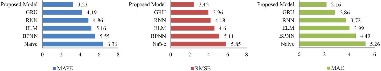
Figure 6 MAPE (%), RMSE (W/m) and MAE (W/m) of developed models on an annual average basis.
Case 2: Comparative research with EEMD based models This scenario uses EEMD preprocessing technique to decompose the global horizontal irradiance data in which generate eight IMFs and one residue. From Table 3, it is observed that for 1-hr ahead solar GHI forecasting, the MAPE obtained by the EEMD-BPNN, EEMD-ELM, EEMD-RNN, EEMD-GRU and the suggested model is ranges from 3.11–6.10%, 2.81%–5.91%, 2.45–5.31%, 2.21–5.12% and 1.91–4.91% respectively; RMSE varies from 2.91–5.91 W/m, 2.41–5.32 W/m, 2.20–5.11 W/m, 1.91–4.20 W/m and 1.21–3.41 W/m respectively and MAE ranges from 2.19–5.10 W/m, 1.85–4.61 W/m, 1.67–4.31 W/m, 1.41–4.01 W/m and 0.91–3.82 W/m respectively. The result shows that suggested model outperforms EEMD based models in all perspectives. Figure 7 shows a comparative analysis of developed models on annual average basis.
Table 3 Performance comparison between proposed model and EEMD models
| MAPE (%) | |||||||
| Models | Winter | Spring | Summer | Monsoon | Autumn | Annual | |
| 1-hr | EEMD-BPNN | 4.21 | 5.21 | 3.11 | 6.10 | 4.10 | 4.54 |
| ahead | EEMD-ELM | 3.91 | 4.81 | 2.81 | 5.91 | 3.21 | 4.13 |
| solar | EEMD-RNN | 3.81 | 4.61 | 2.45 | 5.31 | 3.11 | 3.85 |
| GHI | EEMD-GRU | 3.71 | 4.41 | 2.21 | 5.12 | 2.81 | 3.65 |
| forecasting | Proposed Model | 3.20 | 3.96 | 1.91 | 4.91 | 2.21 | 3.23 |
| RMSE (W/m) | |||||||
| EEMD-BPNN | 3.51 | 4.60 | 2.91 | 5.91 | 3.50 | 4.08 | |
| EEMD-ELM | 3.20 | 4.21 | 2.41 | 5.32 | 2.81 | 3.59 | |
| EEMD-RNN | 3.11 | 4.11 | 2.20 | 5.11 | 2.65 | 3.43 | |
| EEMD-GRU | 2.97 | 3.91 | 1.91 | 4.20 | 2.21 | 3.04 | |
| Proposed Model | 2.51 | 3.31 | 1.21 | 3.41 | 1.83 | 2.45 | |
| MAE(W/m) | |||||||
| EEMD-BPNN | 3.10 | 4.10 | 2.19 | 5.10 | 2.99 | 3.49 | |
| EEMD-ELM | 2.91 | 3.61 | 1.85 | 4.61 | 2.10 | 3.01 | |
| EEMD-RNN | 2.84 | 3.21 | 1.67 | 4.31 | 1.91 | 2.78 | |
| EEMD-GRU | 2.68 | 3.10 | 1.41 | 4.01 | 1.61 | 2.56 | |
| Proposed Model | 2.16 | 2.81 | 0.91 | 3.82 | 1.11 | 2.16 | |

Figure 7 MAPE (%), RMSE (W/m) and MAE (W/m) of developed models on an annual average basis.
Case 3: Assessment of the chosen features In this case, three LSTM models: standalone LSTM, EEMD based LSTM model include all statistical features and EEMD-GA-LSTM model are compared as an evaluation of selected feature. On the basis of loss function, the representative training process on three feature set using 200 epochs for same LSTM network are depicted in Figure 8 When EEMD-GA was included the training loss decrease gradually from 0.00666 for standalone LSTM to 0.00444 for EEMD based LSTM model and 0.00262 when GA wrapper is included.
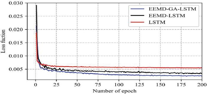
Figure 8 Developed model training procedures were compared.
Table 4 indicates the results of standalone LSTM, EEMD based LSTM and proposed model with respect to MAPE, RMSE and MAE performance criterion.
Table 4 Performance comparison of LSTM models
| MAPE (%) | |||||||
| Models | Winter | Spring | Summer | Monsoon | Autumn | Annual | |
| 1-hr | LSTM | 4.21 | 4.20 | 2.91 | 5.10 | 3.21 | 3.92 |
| ahead | EEMD-LSTM | 3.51 | 4.30 | 2.11 | 5.11 | 2.43 | 3.49 |
| solar | Proposed Model | 3.20 | 3.96 | 1.91 | 4.91 | 2.21 | 3.23 |
| GHI | |||||||
| forecasting | |||||||
| RMSE (W/m) | |||||||
| LSTM | 3.57 | 4.31 | 2.61 | 4.61 | 2.85 | 3.59 | |
| EEMD-LSTM | 2.90 | 3.72 | 1.90 | 4.02 | 1.94 | 2.89 | |
| Proposed Model | 2.51 | 3.31 | 1.21 | 3.41 | 1.83 | 2.45 | |
| MAE(W/m) | |||||||
| LSTM | 2.82 | 3.09 | 1.31 | 4.12 | 2.10 | 2.68 | |
| EEMD-LSTM | 2.43 | 3.11 | 1.10 | 3.91 | 1.21 | 2.35 | |
| Proposed Model | 2.16 | 2.81 | 0.91 | 3.82 | 1.11 | 2.16 | |
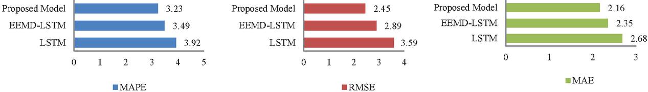
Figure 9 MAPE (%), RMSE (W/m) and MAE (W/m) of developed models on an annual average basis.
5 Discussion
This research performs short term solar irradiance forecasting for the location of Delhi, India. Various experimental analyses are performed in this study to obtain precise model with improved forecasting accuracy. The prediction performance of the proposed model is compared with persistence model, standalone models (BPNN, ELM, GRU, and RNN) and EEMD based models in order to demonstrate its superiority. Finally, based on features evaluation, the prediction results of proposed model is compared to standalone LSTM model and the EEMD-LSTM model which consist all prospective features. From the results, it is clear that the EEMD improve the forecasting accuracy of the standalone models. For a case of summer season, from the table 2 to 3, it is observed that the EEMD improved the RMSE (25.57% for BPNN, 29.32% for ELM, 31.88% for RNN and 34.13% for GRU). However, in case of monsoon season, the accuracy is decreased due to the data instability of the season. But it is concluded that that the EEMD improved the forecasting performance of the standalone model. The similar observations can also be seen for MAPE and MAE. In continuation to these models, the proposed model uses the GA as a feature extraction strategy over the EEMD based models. No doubt from the results, the LSTM model outperforms all standalone models in all terms. The lower RMSE, MAPE and MAE attained by LSTM prove its efficiency over other standalone models and enforce us to utilize this model for further improvements. Therefore, the GA with EEMD process is applied on the LSTM to prove the objective of the study. It is observed that the GA with EEMD credibly improves the forecasting performance of the LSTM. The proposed model improves the results in terms of RMSE, MAPE and MAE compared with all considered models. For a case of annual forecasting, for LSTM and EEMD-LSTM models, the proposed model improves the RMSE (35.36% for LSTM; 21.59% for EEMD-LSTM), MAPE (24.35% for LSTM; 9.01% for EEMD-STM) and MAE (30.99% for LSTM; 10% for EEMD-LSTM). The percentage improvements by proposed model vs non EEMD based models are shown in Figure 10. Similarly, the percentage improvement by proposed model vs. EEMD based models is shown in Figure 11.
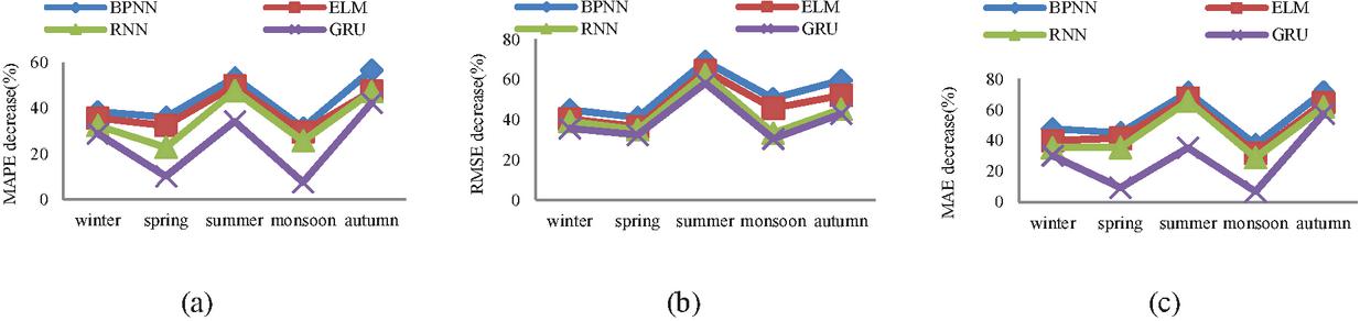
Figure 10 Percentage improvement by proposed model over non-EEMD model.
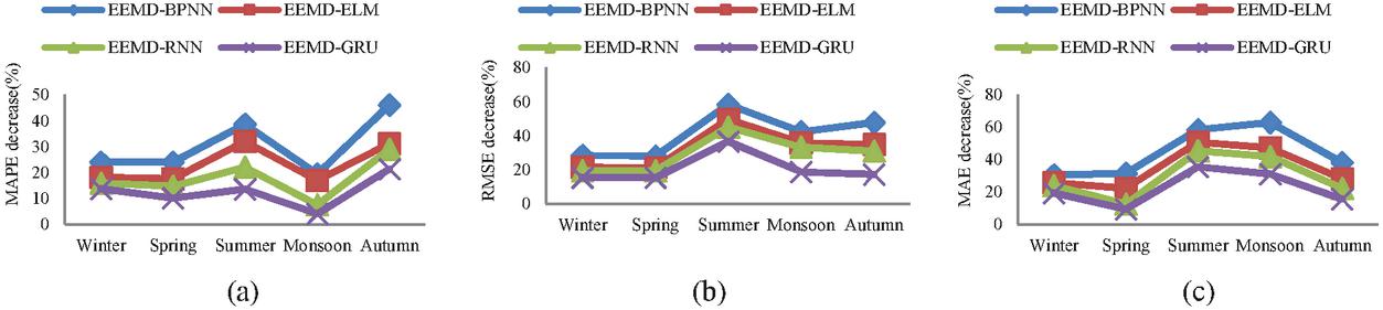
Figure 11 Percentage improvement by proposed model over EEMD model.
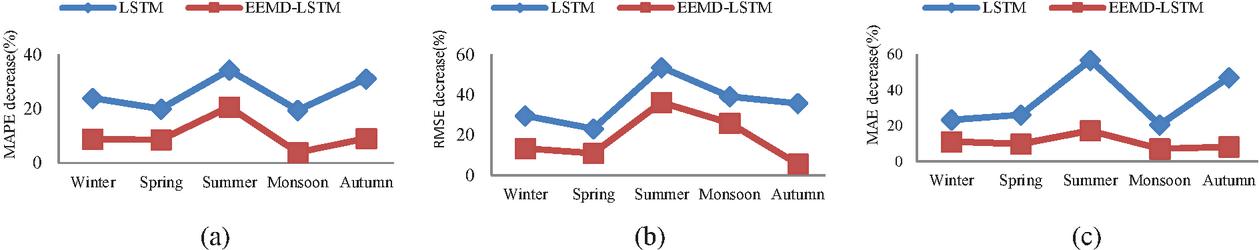
Figure 12 Percentage improvement by proposed model over LSTM and EEMD-LSTM model.
Moreover, for a deeper examination of the findings, Figure 13 provides a graphical representation of real and predicted GHI for four consecutive days (2nd to 5th day) of summer and monsoon season. For clarity, only real and predicted GHI curve of suggested model is shown for selected seasons. From Figure 13 it is observed that substantial fluctuations in the real GHI generate a larger error in the results. For example, smooth curve of summer season indicates the clear environmental circumstances in which easily traceable by the model on the other hand, monsoon season shows substantial fluctuations in the real GHI due to existence of overcast or rainy days making it difficult to trace by the model resulting in maximum inaccuracies. From Figure 13, it can be deduced that if fluctuations in the real GHI is higher, than similarity exist between real and predicted GHI is lower.

Figure 13 Proposed model Performance for the summer and monsoon season.
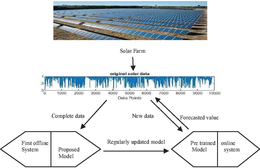
Figure 14 Steps of the distributed system in practical systems for the present framework.
The suggested short-term solar irradiation prediction may be implemented in practical systems utilizing a distributed system (Figure 14), with one system training offline models and the other making online forecasting. The impact of a single future data point on the EEMD spectrum may be small for the largely scaled solar history. As a result, the online system may generate accurate predictions in a short amount of time using pre-trained models. Furthermore, as new records are received, the offline system can update the model at the same time. The model will be transmitted back into the web application for better operations as the volume of data grows significantly.
6 Conclusion
In this study, an ensemble deep learning based architecture is introduced as a method of predicting solar irradiation using a dataset of solar history. When time resolution and recording period of the solar dataset increase, expand the non-linearity in the time series data. The number of IMF will increase dramatically as a result of using EEMD approach on increased time series data. It means more IMF components would result in more untrained data results in which rising of overall training cost. The deep learning model employs to predict the IMF components and forecasting error of each component which them added up to get final error which affect the prediction accuracy of model. To address this problem and to improve forecasting accuracy three major algorithms make up the proposed model: EEMD, GA and LSTM. In the First step, EEMD uses as a preprocessing technique to rectify and extract the inherent characteristics of time series data to obtain an intrinsic mode functions. The well tuned deep learning model and the intuitively picked feature set are synchronized through an optimization method using the paired GA-LSTM technique. The suggested method demonstrates its amazing superiority over conventional models using assessment criteria such as MAE, RMSE and MAPE. To begin, the current model prediction accuracy is increased by 44.96 percent on average when compared to non-EEMD models. On the other hand, when comparing with EEMD approach with other learning prototypes there is a substantial improvement in prediction accuracy of 28.2 percent on average. Furthermore, when comparing the outcomes of the same teaching method with multiple feature sets, the suggested technique is even more powerful from two perspectives: First and foremost it should be possible to use the GA wrapper for selecting features. The length of the model input data is reduced to around a 2/3 of the total population set of features, making it more compact and robust to data fluctuation. Moreover, when compared to all feature and non-feature models, it exceeds them in terms of prediction precision across a wide range of evaluation criteria, with increases of 36.58 percent and 22.74 percent respectively. From all results, it is confirmed that proposed framework is good forecasting model in all perspectives.
References
[1] Vasylieva, T.; Lyulyov, O.; Bilan, Y.; Streimikiene, D. Sustainable economic development and greenhouse gas emissions: The dynamic impact of renewable energy consumption, GDP, and corruption. Energies 2019, 12, 3289.
[2] Gupta, Anuj.; Gupta, Kapil.; Saroha, Sumit.; Solar Irradiation Forecasting Technologies: A Review: Strategic Planning for Energy and the Environemnt.2020: Vol. 39 Iss. 3–4 2020. https://doi.org/10.13052/spee1048-4236.391413
[3] Gupta, Anuj.; Gupta, Kapil.; Saroha Sumit.; A Review and Evaluation of Solar Forecasting Technologies: Materials today proceedings 2021, Volume 47, Part 10, 2021, Pages 2420–2425. https://doi.org/10.1016/j.matpr.2021.04.491
[4] Al-Hajj, R.; Assi, A.; Fouad, M.M. Forecasting Solar Radiation Strength Using Machine Learning Ensemble. In Proceedings of the 7th IEEE International Conference on Renewable Energy Research and Applications (ICRERA), Paris, France, 14–17 October 2018; pp. 184–188.
[5] Gupta A., Gupta K., Saroha S. (2022) Solar Energy Radiation Forecasting Method. In: Agarwal P., Mittal M., Ahmed J., Idrees S.M. (eds) Smart Technologies for Energy and Environmental Sustainability. Green Energy and Technology. Springer, Cham. https://doi.org/10.1007/978-3-030-80702-3\_7
[6] Singla P, Duhan M, Saroha S (2021) A comprehensive review and analysis of solar forecasting techniques. Front Energy. https://doi.org/10.1007/s11708-021-0722-7
[7] Olatomiwa, L.; Mekhilef, S.; Shamshirband, S.; Mohammadi, K.; Petković, D.; Sudheer, C. A support vector machine–firefly algorithm-based model for global solar radiation prediction. Sol. Energy 2015, 115, 632–644.
[8] Fan, J.; Wu, L.; Zhang, F.; Cai, H.; Zeng, W.; Wang, X.; Zou, H. Empirical and machine learning models for predicting daily global solar radiation from sunshine duration: A review and case study in China. Renew. Sustain. Energy Rev. 2019, 100, 186—212.
[9] Gupta A., Gupta K., Saroha S. (2022) Single Step-Ahead Solar Irradiation Forecasting Based on Empirical Mode Decomposition with Back Propagation Neural Network. In: Gupta O.H., Sood V.K., Malik O.P. (eds) Recent Advances in Power Systems. Lecture Notes in Electrical Engineering, vol 812. Springer, Singapore. https://doi.org/10.1007/978-981-16-6970-5\_10
[10] Al-Hajj, R.; Assi, A.; Fouad, M. Short-Term Prediction of Global Solar Radiation Energy Using Weather Data and Machine Learning Ensembles: A Comparative Study. J. Sol. Energy Eng. 2021, 8, 1–38.
[11] Richardson DS, Cloke HL, Pappenberger F (2020) Evaluation of the consistency of ECMWF ensemble forecasts. Geophys Res Lett 47(11). https://doi.org/10.1029/2020GL087934
[12] Perez R, Kivalov S, Schlemmer J, Hemker K, Hoff TE (2012) Shortterm irradiance variability: Preliminary estimation of station pair correlation as a function of distance. Solar Energy 86(8) Pergamon:2170–2176. https://doi.org/10.1016/j.solener.2012.02.027
[13] Piri, J.; Shamshirband, S.; Petković, D.; Tong, C.W.; Rehman, M.H. Prediction of the solar radiation on the earth using support vector regression technique. Infrared Phys. Technol. 2015, 68, 179–185.
[14] Shadab A, Ahmad S, Said S (2020) Spatial forecasting of solar radiation using ARIMA model. Remote Sens Appl Soc Environ 20:100427. https://doi.org/10.1016/j.rsase.2020.100427
[15] Jahani B, Mohammadi B (2019) A comparison between the application of empirical and ANN methods for estimation of daily global radiation in Iran. Theor Appl Climatol 137(1–2):1257–1269. https://doi.org/10.1007/s00704-018-2666-3
[16] Dumitru C-D, GligorA, Enachescu C 9(2016) Solar photovoltaic energy production forecast using neural networks. Procedia Technol 22: 808–815. https://doi.org/10.1016/j.protcy.2016.01.053
[17] Zeng J, Qiao W (2013) Short-term solar power prediction using a support vector machine. Renew Energy 52:118–127. https://doi.org/10.1016/j.renene.2012.10.009
[18] Gupta A., Gupta K., Saroha S. (2022) A Comparative Analysis of Neural Network-Based Models for Forecasting of Solar Irradiation with Different Learning Algorithms. In: Khosla A., Aggarwal M. (eds) Smart Structures in Energy Infrastructure. Studies in Infrastructure and Control. Springer, Singapore. https://doi.org/10.1007/978-981-16-4744-4\_2
[19] Monjoly, Stéphanie; André, Maïna; Calif, Rudy; Soubdhan, Ted (2017). Hourly forecasting of global solar radiation based on multiscale decomposition methods: A hybrid approach. Energy, 119(), 288–298. https://doi:10.1016/j.energy.2016.11.061
[20] Zendehboudi, Alireza; Baseer, M.A.; Saidur, R. (2018). Application of support vector machine models for forecasting solar and wind energy resources: A review. Journal of Cleaner Production, 199, 272–285. https://doi:10.1016/j.jclepro.2018.07.164
[21] Chen, C.-R.; Ouedraogo, F.B.; Chang, Y.-M.; Larasati, D.A.; Tan, S.-W. Hour-Ahead Photovoltaic Output Forecasting Using Wavelet-ANFIS. Mathematics 2021, 9, 2438. https://doi.org/10.3390/math9192438
[22] Qing X, Niu Y (2018) hourly day ahead solar irradiance predictions using weather forecasts by LSTM. Energy 148:461–468. https://doi.org/10.1016/j.energy.2018.01.177
[23] Kumari P, Toshniwal D (2021). Extreme gradient boosting and deep neural network based ensemble learning approach to forecasts hourly solar irradiance. J.Clean Prod 279:123285. https://doi.org/10.1016/j.jclepro.2020.123285
[24] Zang H, Liu L, Sun L, Cheng L, Wei Z, Sun G (2020b) Short term global horizontal irradiance forecasting based on a hybrid CNN-LSTM model with spatiotemporal correlations. Renew Energy 160:26–41. https://doi.org/10.1016/j.renene.2020.05.150
[25] Zang H, Cheng L, Ding T, Cheung KW,Wei Z, Sun G (2020a) Day ahead photovoltaic power forecasting approach based on deep convolution neural networks and meta Int J Electr power Energy Syst 118:105790. https://doi.org/10.1016/j.ijepes.2019.105790
[26] Wang F, Yu Y, Zhang Z, Li J, Zhen Z, Li K (2018) Wavelet decomposition and convolution LSTM networks based improved deep learning model for solar irradiance forecasting. Appl Sci 8(8):1286. https://doi.org/10.3390/app8081286
[27] Gao B, Huang X, Shi J, Tai Y, Xiao R (2019) Predicting day-ahead solar irradiance through gated recurrent unit using weather forecasting data. J. Renew Sustain Energy 11(4): 043705. https://doi.org/10.1063/1.5110223
[28] Fischer T, Krauss C (2018) Deep learning with long short-term memory networks for financial market predictions. Eur J Oper Res 270(2): 654–669. https://doi.org/10.1016/j.ejor.2017.11.054
[29] Gao B, Huang X, Shi J, Tai Y, Zhang J (2020) Hourly forecasting of solar irradiance based on CEEMDAN and multi-strategy CNN-LSTM neural networks. Renew Energy 162:1665–1683. https://doi.org/10.1016/j.renene.2020.09.141
[30] Huimin Z, Meng S, Wu D, Xinhua Y. A new feature extraction method based on EEMD and multi-scale fuzzy entropy for motor bearing. Entropy 2016; 19(1):14.
[31] Prasad, Ramendra; Ali, Mumtaz; Kwan, Paul; Khan, Huma (2019). Designing a multi-stage multivariate empirical mode decomposition coupled with ant colony optimization and random forest model to forecast monthly solar radiation. Applied Energy, 236, 778–792. doi:10.1016/j.apenergy.2018.12.034
[32] Qin Q, Lai X, Zou J. Direct multistep wind speed forecasting using LSTM neuralnetwork combining EEMD and fuzzy entropy. Appl Sci 2019; 9(1).
[33] http://delhitourism.gov.in/delhitourism/aboutus/seasons\_of\_delhi.jsp
[34] Huang NE, Shen Z, Long SR, Wu MC, Shih HH, Zheng Q, et al. The empiricial mode decomposition and the Hilbert transform for nonlinear and non-stationary time series analysis. Proc A 1998:454(1971): 903–995.
[35] Wu Z, Hunag NE, Ensemble empirical mode decomposition: a noise-assisted data analysis method. Adv Adapt Data Anal 2009:01(01):1–41.
[36] Hochreiter S, Schmidhuber J. Long short-term memory. Neural Comput 1997;9(8):1735–1180.
[37] Zang H, Liu L, Sun L, Cheng L, Wei Z, Sun G (2020b) Short-termglobal horizontal irradiance forecasting based on a hybrid CNNLSTM model with spatiotemporal correlations. Renew Energy 160:26–41. https://doi.org/10.1016/j.renene.2020.05.150
[38] Huang C, Wang L, Lai LL (2019) Data-driven short-term solar irradiance forecasting based on information of neighboring sites. IEEE Trans Ind Electron 66(12):9918–9927. https://doi.org/10.1109/TIE.2018.2856199
[39] Bedi J, Toshniwal D (2019) Deep learning framework to forecast electricity demand. Appl Energy 238:1312–1326. https://doi.org/10.w1016/j.apenergy.2019.01.113
[40] Singla, P., Duhan, M. & Saroha, S. An ensemble method to forecast 24-h ahead solar irradiance using wavelet decomposition and BiLSTM deep learning network. Earth Sci Inform 15, 291–306 (2022). https://doi.org/10.1007/s12145-021-00723-1
Biographies

Anuj Gupta received the B.Tech in Electronics and Communication Engineering from Kurukshetra University, M.Tech in Electronics and Communication Engineering from Kurukshetra University, Kurukshetra. Presently he is Assistant Professor in EEE Department at Asia Pacific Institute of Information Technology, Panipat and pursuing Ph.D. in the area of solar irradiance forecasting from Electronics and Communication Engineering Department, Maharishi Markandeshwar University, Mullana-Ambala, India. His research area is deregulated electricity market, solar irradiance forecasting. He has more than seven years teaching and research experience.

Kapil Gupta received his B.E. (HONS) degree in Electronics & Communication engineering in 2003 from Rajasthan University and M.E. (HONS) degree in Digital Communication from MBM Engineering College Jodhpur, Rajasthan in 2008. He earned Ph.D. degree in 2013 from MITS University, Rajasthan. Presently he is Associate Professor in the Department of Electronics and Communication Engineering, M.M.E.C, Maharishi Markandeshwar (Deemed to be University) Mullana-Ambala and has more than 15 years of experience in teaching. His research interests are in solar irradiance forecasting, Wireless Sensor Networks, Wireless Communication, Diversity Techniques and Error Correction Coding.

Sumit Saroha is currently working as Assistant Professor in the Depart- ment of Electrical Engineering, Guru Jambheshwar University of Science & Technology, Hisar, India. He received Ph.D. in the area of forecasting issues in present day power systems. His research interests are transformer design, electricity markets, electricity forecasting, neural networks, wavelet transform, fractional order systems and Multi agent system.
Strategic Planning for Energy and the Environment, Vol. 41_3, 255–280.
doi: 10.13052/spee1048-5236.4132
© 2022 River Publishers