Correlation Analysis and Monitoring Method of Carbon Emissions in the Steel Industry Based on Big Data
Wang Yang1, Gao Yi2,*, Zou Zhiyu3, Chen Yue2, Xudong Wang1, Luo Shuai2, Liu Ning1, Zhou Jin2 and Yan Dawei2
1State Grid Tianjin Electric Power Company, Tianjin 300010, China
2State Grid Tianjin Economic and Technological Research Institute, Tianjin 300171, China
3Key Laboratory of Smart Grid of Ministry of Education, Tianjin University, Tianjin 300072, China
E-mail: wywdm20@126.com; 13502076821@163.com; zzy_zy@126.com; yuechen2011@163.com; tjwangxudong@sina.com; hdln512@126.com; k_zj@163.com; houruosong@126.com
*Corresponding Author
Received 09 March 2023; Accepted 17 April 2023; Publication 18 December 2023
Abstract
Excessive carbon emissions will lead to catastrophic consequences such as global warming and rising oceans and will also have a serious negative impact on the human food supply and living environment. The steel industry is characterized by high pollution, and about 18% of China’s carbon emissions come from the steel industry. The ‘double carbon’ strategy has brought important tasks and severe challenges to China’s steel industry. With a view to evaluating the achievements of carbon emission control, carbon emission monitoring systems at home and abroad have been continuously established and improved. For the steel industry, accurate and efficient carbon monitoring technology has a guiding role in guiding energy conservation and carbon reduction. Traditional carbon emission accounting methods have some problems, such as long cycles and poor data quality, which restrict the improvement of the lean level of carbon emission monitoring management. Firstly, this paper investigates and analyzes the productive process and carbon emission process of the steel industry and constructs an entropy weight-grey correlation -TOPSIS analysis method for the correlation between carbon emissions and influencing factors. Based on the above content, a carbon emission monitoring method based on multiple influencing factors is put forward, and the high monitoring accuracy of the model is proved by taking the Tianjin steel industry as an example. The results show that information mining of relevant data can strikingly increase the accuracy of carbon emission monitoring in the steel industry.
Keywords: Big data, carbon emissions, carbon emission monitoring, energy consumption, steel industry.
1 Introduction
In 2018, a report detailing the eight major catastrophic risks brought about by changing climate and indicating the urgency of climate control has published by the United Nations Intergovernmental Panel on Climate Change (IPCC). In response to the challenges posed by environmental pollution, more and more countries have turned “carbon neutrality” into a national strategy. As of now extra than one hundred and twenty nations around the world have pledged to achieve carbon neutrality by the middle of the 21st century, and more than 110 countries have proposed to update their independent contribution goals by 2030. In September 2020, Chinese President Xi Jinping introduced that China will endeavor to meet the “carbon peak” before 2030 and “carbon neutrality” before 2060, indicating China’s ambition to participate in global climate governance. China is the greatest steel producer and the biggest steel consumer in the whole world. In 2021, China had a steel output of 1.03 billion tons, accounting for 53% of the world’s total. High output also brings about high air pollution and high energy consumption. About 33.8% of the total industrial CO emissions come from the steel industry. It is a key source of CO emissions in China. So as to cope with global climate change and environmental pollution, the “double carbon” strategy poses a tough challenge to the further development of China’s steel industry [1]. As the most significant carbon emission industry in China’s manufacturing department, the steel industry must complete the green and low-carbon transformation as soon as possible and complete the increasingly urgent carbon emission reduction task. To accomplish the goal of carbon neutrality and emission reduction, the three links in the whole process of steel production, i.e., the start-process-terminal [2], should participate in the advance of low-carbon technologies, among which accurate and timely carbon emission measurement is an indispensable foundation for promoting the green transformation of China’s steel industry.
Carbon emission monitoring and accurate accounting are the basis for the government to carry out carbon emission responsibility sharing and carbon trading market, and they are also the key to stimulating the green-oriented transition of enterprises and supporting the scientific decision-making of coordinated development among energy, economy, and environment. At present, mature carbon emission accounting methods include the Emission Factor Approach, Carbon Material Flow Analysis, and Continuous Emission Monitoring. The Emission-Factor Approach is broadly used, and this method uses the default emission factors of IPCC and fuel consumption to calculate carbon emissions [3]. However, there are many types of carbon emission sources in the steel industry, and the characteristics of different enterprises are different, which leads to a big difference between the default parameter and the actual value of the carbon emission factor, so it is difficult to guarantee the accuracy of carbon emission monitoring. The Carbon Material Flow Analysis calculates carbon emissions by measuring the input and output of carbon, which requires high precision for data such as product scheme, process flow, production scale, and raw material consumption, and it is difficult to realize. Continuous Emission Monitoring, generally, a carbon emission monitoring module is installed in the Continuous Emission Monitoring System (CEMS), and the emission of carbon dioxide is directly measured by continuously monitoring the concentration and flow rate of carbon dioxide, which has good data timeliness but high cost [4]. In addition, there are many kinds and quantities of operation data related to carbon emission in the steel industry, and the existing emission monitoring system lacks data analysis means, so it is difficult to mine and utilize the correlation information contained in each operation data.
To enhance the real-time accuracy of carbon emission measurement and provide a data basis for further carbon emission reduction, plenty of scholars and experts have carried out research in the field of carbon emission in the steel industry. Reference [5] analyzes the relationship between the economy and CO emissions in the steel industry by the three-stage least square model, which shows that there is a two-way causal relevance between economy and CO emissions in most steel enterprises. Reference [6] analyzes the influence of different factors on CO emission in the steel industry by using historical data on the steel industry and gives some policy suggestions. Reference [7] relates carbon emission and energy consumption and puts forward the optimization method of the production process in the steel industry. Li Xinchuang etc. studied and analyzed the carbon emission system standards both at home and abroad based on the carbon emission status of the steel industry [8]. Wang Xuying etc. comprehensively considered the economy, energy, low-carbon technology application, and other aspects and carried out research on the CO emission peak path in the steel industry based on scenario analysis [9]. However, the above research failed to combine carbon emission monitoring with the specific features of the steel industry. On the basis of now available relevant data and supporting facilities, how to consider the carbon emission characteristics of the steel industry production process and complete the accurate and practical carbon emission of the steel industry still need further research.
To solve the above problems, this paper investigates the production process of the steel industry and analyzes the range of carbon emission influencing factors in the steel industry. This paper analyzes the correlation between different influencing factors and carbon emissions in the steel industry based on the entropy weight-grey correlation -TOPSIS model so as to screen the input of the model and avoid data redundancy to reduce the accuracy of carbon emissions measurement. Long short-term memory (LSTM) and Grey model (1, N) (GM(1, N)) are used to further extract effective information from the long-time series data of carbon emissions and selected influencing factors and complete the carbon monitoring of the steel industry based on correlation. The carbon emission monitoring method described in this paper considers the characteristics of the steel industry and takes full advantage of the existing database. Figure 1 shows the overall framework of the method.
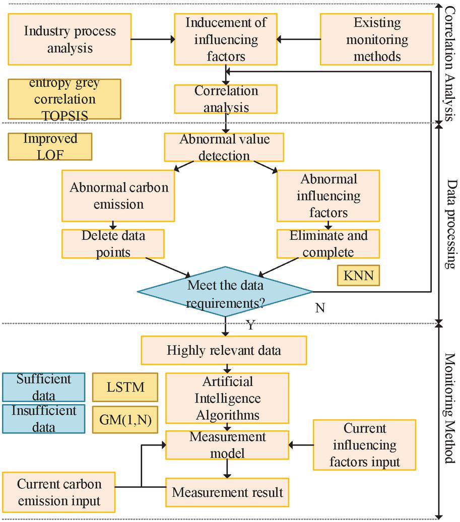
Figure 1 Overall framework of the method.
2 Calculation Model Based on Analysis of Carbon Emission Characteristics in the Steel Industry
2.1 Analysis of the Steel Industry Production Process
The current carbon emission monitoring method can’t comprehensively consider the inner and outer factors of carbon emission in the steel industry. Therefore, this work first studies the production processes and carbon emission links in the steel industry.
The productive process of the steel industry includes five links: coking, sintering, ironmaking, steelmaking, and steel processing:
The coking process flow is shown in Figure 2. After coal blending according to the proportion, it is heated to 9501050C in a coking furnace under the condition of isolated air and dried at high temperature to make coke and crude gas. The CO emission from the coking process is mainly caused by the combustion of fuel in the coking process, and some CO emissions are caused by the escape of coke oven gas and gaseous chemical products in the production process.
The sintering process flow is shown in Figure 3. The prepared raw materials, such as iron, fuel, flux, substitutes, etc. are proportioned, mixed, and granulated according to a certain proportion, laid on the trolley of the sintering machine, and ignited under negative pressure [10]. After ignition, the sintered materials are partially softened and melted by the high temperature generated by the combustion and oxidation of iron-oxygen minerals, resulting in physical and chemical reactions, forming a blocky burden with sufficient strength and granularity, and finally, the sintered ore is obtained after crushing and screening. The emission of CO in this process basically comes from the combustion of fuel in the sintering material and the CO produced in the process of flux sintering.
The ironmaking process flow is shown in Figure 4. The blast furnace process has the highest energy consumption in China’s steel production process, accounting for more than 50% of the whole process’s energy consumption [11]. Carbon dioxide emissions from the ironmaking process mainly come from the emissions from the combustion of coke or other fuels, the emissions from the consumption of different carbon-containing raw materials same as purchased ferroalloy, and the emissions from the decomposition of flux.
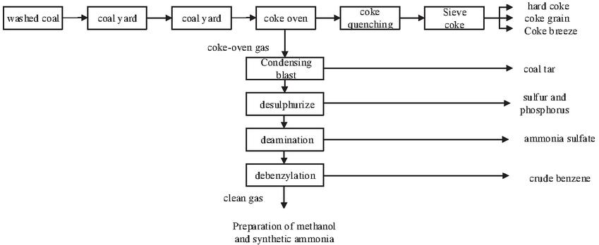
Figure 2 Coking process flow.
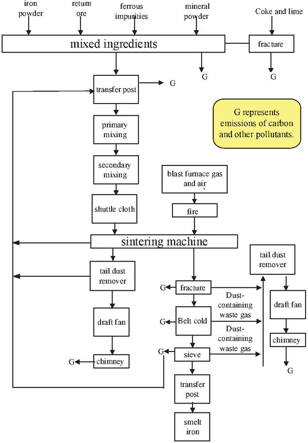
Figure 3 Sintering process flow.
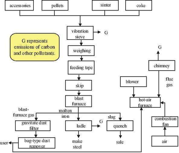
Figure 4 Ironmaking process flow.
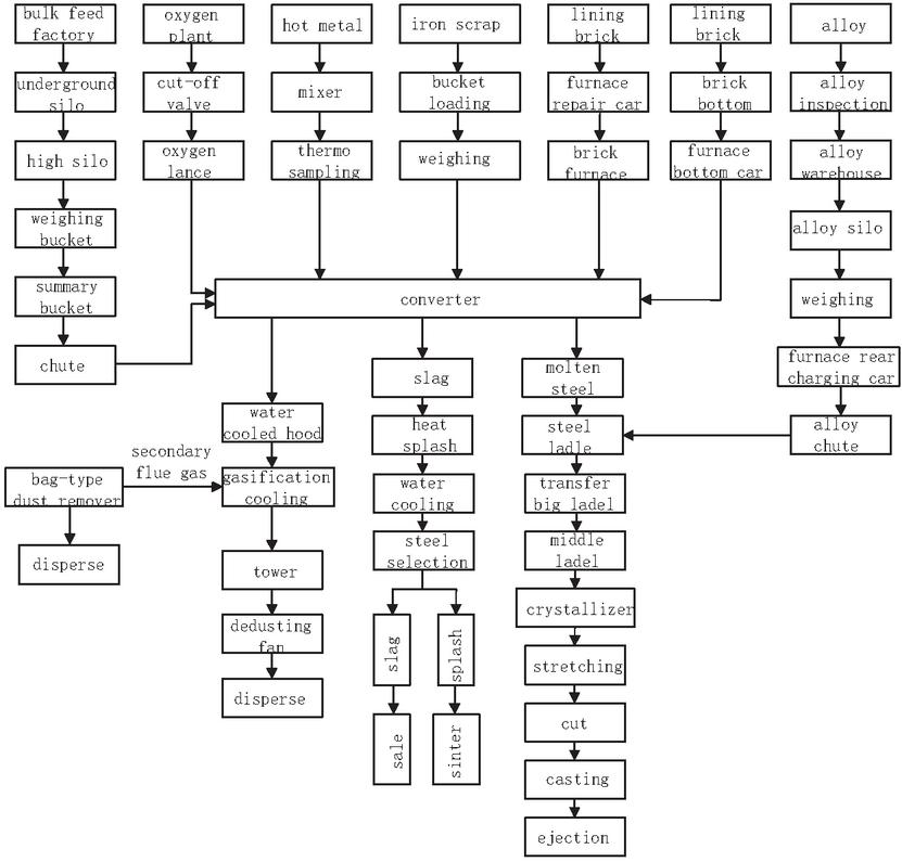
Figure 5 Steelmaking process flow.
The steelmaking process flow is shown in Figure 5. The steelmaking process is mainly composed of raw material storage and transportation, converter smelting, converter flue gas purification, vaporization cooling, slag treatment, continuous casting, etc. According to the proportion, scrap steel and molten iron are poured into the converter, slag-making materials such as quicklime are added, and oxygen is blown into the furnace top to oxidize impurity elements such as silicon, sulfur, carbon, manganese, and phosphorus in molten iron into various oxides, forming steel slag or gas, which is then removed. Carbon dioxide emission from the steelmaking process mainly comes from fuel combustion and carbon oxidation in molten iron.
The steel processing procedure flow is shown in Figure 6. There are many forms of steel processing, and steel rolling is the main form of iron and steel joint enterprises. The energy consumption of steel processing is large, and the CO emission mainly comes from the purchase of electricity.
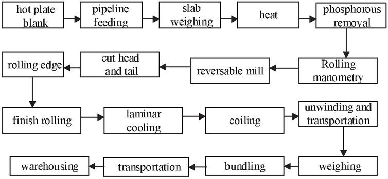
Figure 6 Steel processing procedure flow.
2.2 Traceability of Carbon Emissions in the Steel Industry
It can be concluded by the production process mentioned above that the total amount of CO emissions from steel production enterprises is considered as the summation of fossil fuel combustion emissions, industrial production process emissions, emissions implicit by the net purchase of electric power by enterprises, and the implied emissions from carbon sequestration products are deducted, which is calculated according to (1).
| (1) |
where equals the summation of emissions from the combustion of diverse fuels consumed by the industry in the accounting period:
| (2) |
where is the CO emission factor of the th fossil fuel, and is the consumption of the th fossil fuel in the accounting period, and the calculation formula is as follows:
| (3) |
where represents the average heat value of the th fossil fuel and represents the net consumption of the th fossil fuel in the accounting period.
The carbon dioxide emission factor of fossil fuels is calculated as (4):
| (4) |
where represents the C element content per unit heat value of the th fossil fuel and represents the carbon oxygenation efficiency of it.
CO emissions in industrial processes come from solvents, electrodes, and raw materials.
| (5) |
The CO implied by the purchase of net electricity comes from the carbon produced by the power providers.
For carbon-fixing products such as crude steel, gas, methanol, etc., the solidified CO is not emitted within the boundary of the enterprise but is implicitly emitted in the subsequent process of the product, and the corresponding carbon emissions should be deducted.

Figure 7 Carbon emission composition of Tianjin steel industry.
3 Correlation Model of Carbon Emission Data in the Steel Industry
3.1 Calculation Method of Carbon Emissions Based on Influencing Factors
According to investigation and research, the carbon emission structure of the Tianjin steel industry is shown in Figure 7, and the proportion of purchased electric power is small. The carbon emission monitoring method based on electricity alone is not suitable for the steel industry. For this reason, the historical data of the economy, output, etc. are incorporated into the carbon emission monitoring model, i.e.
| (6) |
where represents carbon dioxide emission forecast, , and represent the historical data of electricity, economy, and production, respectively. Other relevant historical data should also be included in the model.
Aiming at the steel industry, this work analyzed and summarized the influencing factors of carbon emissions in the steel industry and constructs an energy big data demand catalog for carbon monitoring services. The influencing factors are mainly considered from three aspects: (1) Macro factors, e.g., energy consumption and economic yield; (2) External driving factors, including investment scale and diverse factors that indirectly influence carbon emissions; (3) Important factors in each link of the steel industrial production process. The following table lists the indicators and meanings of some influencing factors of carbon emissions in the steel industry.
Table 1 Index of influencing factors of the steel industry
| Variable | Symbol | Meaning |
| Value Added | VA | The added value of the steel enterprise |
| Output Carbon Intensity | OCI | Carbon emissions per unit of added value |
| Energy Intensity | EI | Energy consumption per unit output value |
| Electricity Consumption | EC | Electricity consumption data of the steel industry |
| Green Electricity Proportion | GEP | The proportion of clean energy generation |
| Enterprise Scale | SCL | The proportion of production value in the region |
| Product Structure | PS | The proportion of crude steel output |
| Technical Competence | TEC | Number of related patented technologies of steel |
Some influencing factors are specifically described as follows:
Energy Intensity: Energy intensity reflects the comprehensive utilization efficiency of energy in different countries, regions, and enterprises. When the total output value is constant, the stronger the energy consumption intensity, the larger the carbon emissions of enterprises [12]. However, the energy intensity is also related to the environmental technical efficiency, so the correlation between the energy intensity and the emissions intensity is still unclear.
Enterprise Scale: The enterprise scale represents the concentration of human, material, and financial resources, which is a key factor affecting carbon emissions. However, enterprise scale has a double-sided influence on carbon emissions. On the one hand, the bigger the scale of enterprises, the greater the efficiency of resource integration and utilization; on the other hand, when the scale of enterprises exceeds a certain threshold, the carbon emission efficiency hardly increases.
Product Structure: Steel products mainly include pig iron, crude steel, and steel products, and the amount of carbon dioxide emitted by different products is different. Among them, the production of crude steel needs to consume a lot of fossil energy, while the production of steel products mainly consumes electric energy and emits less carbon dioxide. Therefore, the carbon dioxide emission rate is closely related to the product structure.
Technical Competence: From the dynamic trend of carbon emission efficiency in the steel industry in recent years, it can be found that the output of carbon emissions is largely affected by the level of technology. Through the improvement and perfection of technology, technological progress can bring economic development on the one hand, and reduce energy input and pollution emissions on the other hand [13].
3.2 Correlation Analysis of Influencing Factors
An influencing factors quantitative analysis model based on entropy grey correlation TOPSIS is constructed. This work uses the entropy weight method to calculate the weight of influencing factors of carbon emission., which effectively reduces the subjective impact and makes the evaluation results more authentic [14]; The original TOPSIS method is usually expressed by linear piecewise function, but its disadvantage is that it cannot reflect the possible nonlinear relationship among the elements in the research object. The introduction of the grey correlation degree can effectively correct this defect of the TOPSIS method [15].
In the process of constructing the evaluation index system, different influencing factors are different in direction and order of magnitude. The data of positive and negative indexes are standardized through (7) and (8) respectively.
| (7) | ||
| (8) |
In the matrix with types of influencing factors, is the index data of influencing factors in row and column before standardization and is the result data after standardization.
The weights of the influencing factors are computationally acquired by solving the information entropy of the index. The information entropy of the influencing factor is denoted as , and its calculation formula is as follows:
| (9) | |
| (10) | |
| (11) |
where is the contribution of index data to influencing factor .
Calculate the weight of the influencing factor by (10).
| (12) |
A new matrix can be obtained by multiplying the entropy weight of each influencing factor by the matrix obtained by standardization. The ideal positive solution set and negative solution set are respectively the set consisting of the maximum and minimum values of all influencing factors in the matrix that is weighted and normalized.
The grey correlation coefficient matrix between the influencing factors and positive and negative ideal solutions is recorded as and . The calculation formulas of elements and in the matrix are shown in (3.2) and (3.2) respectively.
where represents the resolution coefficient and satisfies , the smaller the value, the more significant the resolution effect. For the convenience of calculation, this paper takes as 0.5.
Calculate the grey correlation degree and between each influencing factor and ideal positive and negative solutions as follows:
| (15) | ||
| (16) |
The grey correlation degree and , Euclidean distance and are processed dimensionless in turn and merged:
| (17) | ||
| (18) | ||
| (19) |
Finally, the relative closeness of each influencing factor is determined, and its calculation formula is as follows:
| (20) |
where is the relative closeness of the influencing factor, the larger the value, the stronger the correlation between the influencing factor and carbon emissions; On the contrary, the influence factors with small value have a weak correlation with carbon emissions, which may affect the accuracy of the model.
4 Dynamic Monitoring of Carbon Emissions Based on Correlation Model
4.1 Outlier Detection Based on Correlation
In the process of data acquisition, transmission, and storage, it is inevitable that data will be abnormally missing due to uncontrollable factors such as abnormal communication. The abnormality of the sample leads to the destruction of the data correlation and the deviation of the model results, which brings great difficulties to the follow-up carbon emission monitoring and analysis. Therefore, the effective elimination of abnormal data is an important prerequisite to achieving high-precision carbon emission monitoring in key industries.
LOF (Local Outlier Factor) is a commonly used algorithm for detecting outliers. The algorithm computes the outlier index of all data points to determine the outlier point set and usually selects some points with the largest outlier index as outliers. LOF algorithm based on distance calculation is defined as follows:
Definition 1 (k-distance): the k-distance of the data object is defined as the distance from the nearest th point in the data set to the data object , denoted by .
Definition 2 (k-distance neighborhood): The points set within the circle with the point as the center and as the radius is the k-distance neighborhood, denoted by .
Definition 3 (reachable distance): , the reachable distance between the data point and data point is the maximum value of and , i.e.
| (21) |
where means the distance between the data point and the data point , as shown in Figure 8.
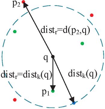
Figure 8 Various distances of LOF.
Definition 4 (local reachable density): The reciprocal of the mean value of the reachable distance of all points in the k-distance neighborhood of the point is called the local reachable density of , i.e.
| (22) |
Definition 5 (local outlier factor): The value of the average local reachable density of the neighbors of divided by the local reachable density of , i.e.
| (23) |
Because the volatility of multidimensional data with different eigenvalues is quite different, in practical application, the traditional LOF tends to treat the normal data with a large characteristic fluctuation as an abnormal value, or it can’t identify the abnormal data because of a small characteristic fluctuation. Therefore, this paper proposes an improved LOF algorithm.
The traditional LOF distance calculation adopts Euclidean distance, and the calculation method of n-dimensional data is:
| (24) |
This calculation method doesn’t take into account the different dimensions of multidimensional data [16], so this paper uses Mahalanobis distance to calculate:
| (25) |
where is the covariance matrix of multidimensional variables.
According to the volatility of different data, the relative closeness of influencing factors is taken as the calculation weight of each influencing factor in LOF. Based on a detailed data analysis, it was found that normal signals collected from the research subjects often display similar data feature distributions. Incorporating weights further reduces the distances between the data points, resulting in feature differences between normal signals that tend towards, or equal to, zero. This can lead to a situation whereby the calculation of local outlier factor (LOF) produces an issue in which the locally reachable density approaches infinity [17]. For this reason, an exponential function is introduced to map the distance. The weighted distance calculation formula is as follows:
| (26) |
The monitored outliers are divided into two situations, which are treated differently: (1) When the outliers are the influencing factors, the outliers are eliminated, and the K-Nearest Neighbor (KNN) algorithm is used to complete the data. KNN considers the continuity of time series data and uses the weighted average of recent observation points as the filling value. (2) When the outlier is carbon emission data, completing the data is equivalent to making an inaccurate prediction, but it will reduce the accuracy of the model, so we choose to delete the data point [18].
4.2 Carbon Emission Monitoring Based on Dynamic LSTM
With the advancement of time, when new data enter the training set, in order to avoid model redundancy or over-fitting caused by too much data, it is essential to control the scale of the training set reasonably. To ensure the uniformity of data in time series, the maximum interval driving strategy eliminates the oldest data when adding new data. That is, it realizes the translation of training data in time. This method is simple to realize, but it will not be of great help to the improvement of model accuracy.
The strategy of minimum error rate driving means that the retained sample is the sample with the minimum error rate when certain data is eliminated. This method of elimination needs to traverse all the data to try to eliminate and then compare the training results so as to obtain the final data to be eliminated. When the data scale is very large, it will take too long and have low practicability.
In this paper, the hybrid driving strategy is adopted to update the data. Considering the advantages of the two strategies, the data with small or even negative contributions to the model is eliminated while keeping the time uniformity of the data as much as possible.
LSTM has obvious advantages in processing time series data [19]. In this paper, LSTM is used to realize carbon emission monitoring based on influencing factors. The structure is shown in Figure 9:
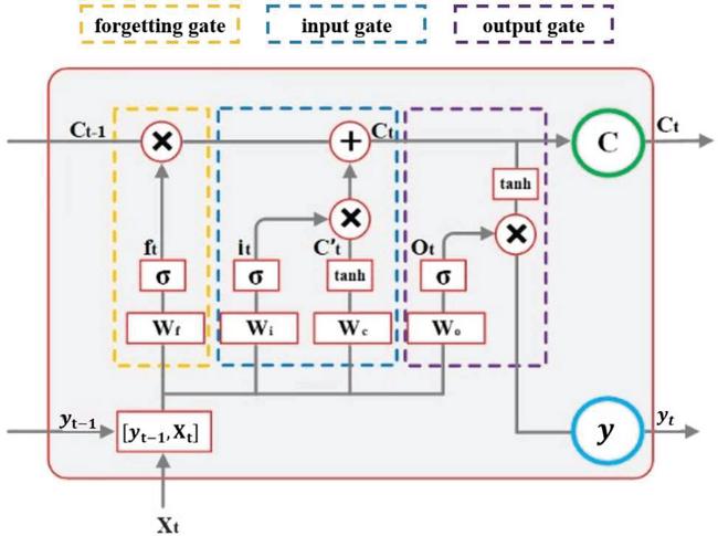
Figure 9 Structure of LSTM.
In LSTM, is the weight matrix of each unit and is the corresponding bias, which together determines the information conversion in the control gate and Cell [20].
This part of the operation is determined by the forgetting gate and Sigmoid function in it. The forgetting gate analyzes the information in historical carbon emission data and influencing factors and finally determines which information is forgotten by , and the output value of is between 0 and 1, where 0 means that all the information in is not retained, and 1 means that all of it is kept. Its calculation equation is as follows:
| (27) |
After that, LSTM will prepare to update the information in the Cell. First, the input gate reads the information in and , then decides which information needs to be updated by again. Then, the function is used to select the candidate information in and that may need to be written in .
| (28) | ||
| (29) |
The current cell information is obtained by adding the old information selected and retained by the forgetting gate and the new information selected from the candidate information by the input gate, as follows:
| (30) |
Finally, the updated cell information and the input feature together determine the output of LSTM and get the real-time carbon emission monitoring data of the steel industry.
| (31) | ||
| (32) |
When there are many outliers in data, the available data may be reduced, and the accuracy of the LSTM algorithm will be reduced [21]. In this case, the GM (1, N) prediction model can be used to accumulate the series to complete the effective monitoring of carbon emissions. GM(1, N) has obvious advantages in small sample models [22], and its definition is as follows. Let the original data sequence be , and the sequence generated by one-time accumulation be . Equation (33) is the mathematical model of GM(1, N). Where is the system developing coefficient, is called the driving term, is called the driving coefficient, and is called the parameter sequence of the model. Equations (33) and (34) are called the whitening equation of the model.
| (33) | |
| (34) |
Then the least square estimation of the parameter sequence satisfies: . GM(1, N) model is able to synchronously reflect the effect of influencing factors on the system behavior feature sequence depending on the model structure and its own dynamic characteristics and can predict the system behavior feature sequence on the premise of knowing the future change trend information of driving factors [23].
5 Case Study
In this paper, taking Tianjin as an example, firstly, based on entropy weight-grey correlation -TOPSIS, the correlation analysis of influencing factors is carried out, and the results are shown in Figure 10. The data in the example are mainly provided by State Grid Tianjin Electric Power Co., LTD, and some data are taken from Tianjin Statistical Yearbook. Note that the output result of correlation analysis is in the range of 1 to 1, in which the nearer to 1, the closer the negative correlation; the nearer to 1, the closer the positive correlation; and 0 means no correlation.
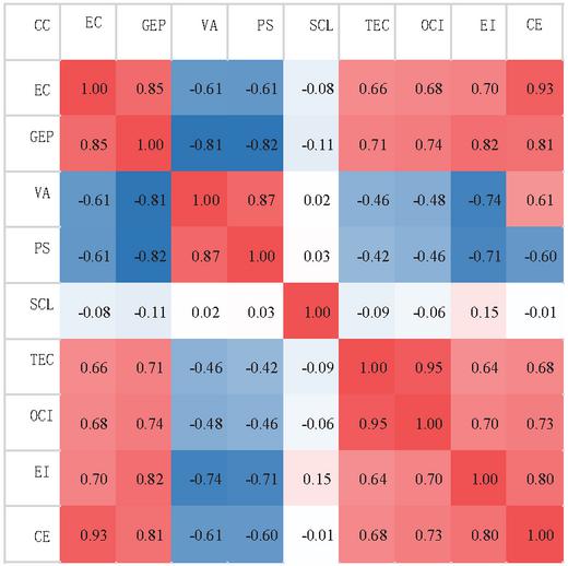
Figure 10 Correlation analysis of influencing factors of carbon emissions in the steel industry.
For the steel industry in Tianjin, the scale of enterprises has little correlation with carbon emissions, and the scale of enterprises has little correlation with other influencing factors too. Except for the scale of enterprises, carbon emissions are closely related to other influencing factors, among which, it is negatively related to product structure and economic output, while it is positively related to other factors. Therefore, it is considered that Enterprise Scale is a redundant variable in carbon emission measurement of steel industry and should be deleted. Finally, Value Added, Output Carbon Intensity, Energy Intensity, Electricity Consumption, Green Electricity Proportion, Enterprise Scale, Product Structure and Technical Competitiveness are selected as important influencing factors to join the model training.
The historical data of carbon emissions of the Tianjin steel industry from 2006 to 2019 and other influencing factors except enterprise scale were added to LSTM model training, and as a comparison, auto-regressive moving average model (ARMA), Support Vector Machine (SVM) and ridge regression were used to calculate carbon emissions, with the results shown in Figure 11:
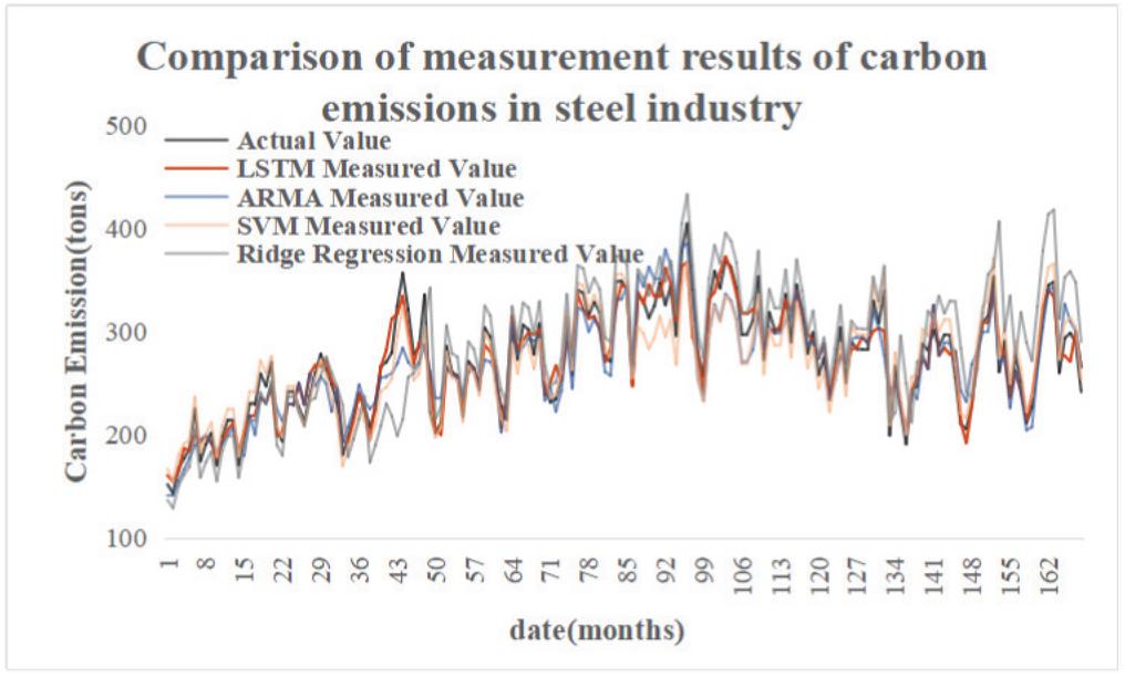
Figure 11 Comparison of measurement results of carbon emissions in the Tianjin steel industry.
The Mean Absolute Percentage Error (MAPE), Mean Absolute Error (MAE) and Mean Square Error (MSE) of each algorithm in the example are shown in Table 2.
Table 2 Calculation error of different algorithms
| Algorithms | MAPE/% | MAE/(tonsCO) | MSE/(tonsCO) |
| LSTM | 4.71 | 15.23 | 260.50 |
| ARMA | 6.42 | 17.30 | 444.42 |
| SVM | 5.19 | 16.47 | 280.25 |
| Ridge regression | 10.0 | 28.01 | 1324.59l |
The conclusions can be summarized as follows:
(1) The carbon emission of the steel industry is large, but the fluctuation of carbon emission is relatively stable, and the LSTM measurement model proposed in this word is able to get a superior accuracy of carbon emission measurement. Among them, the root mean square error of carbon emission measurement is 18.89 tons/CO, the average absolute error is 15.23 tons/CO, and the measurement accuracy is 97.76%. And the measured carbon emission curve is basically consistent with the fluctuation trend of the real carbon emission curve;
(2) The overall accuracy of the carbon emission measurement model of the steel industry based on big data is high, which indicates that the model can be more competent and complete the task of carbon emission measurement of the steel industry. In this example, the LSTM algorithm has lower errors than other algorithms in all aspects. This indicates that the LSTM algorithm is more suitable for carbon emission measurement based on big data.
6 Conclusion
Carbon emissions produced by the steel industry account for a large part of carbon emissions in China. This paper investigates and analyzes the production process of the steel industry and studies the influencing factors of carbon emissions. In this paper, the evaluation model based on entropy weight-grey correlation -TOPSIS is used to analyze the correlation of different carbon emission influencing factors, and it is concluded that in the steel industry CO emissions data is highly correlated with data such as electricity and economy, while the correlation with the scale of the enterprise is weak.
Aiming at the carbon emission of the Tianjin steel industry, this work adds the influential factors with strong correlation into the calculation model, and the calculation accuracy of the obtained model is over 95%, which can fulfill the requirements of carbon emission calculation of the steel industry. Because of data security and privacy, this paper only establishes the correlation model between influencing factors and carbon emissions based on available data, so how to establish a comprehensive correlation monitoring model of carbon emissions needs further study. In general, apart from the power data, the carbon emissions of the steel industry are highly correlated with many factors. Mining and making full use of relevant data can significantly improve the accuracy of carbon emission monitoring.
Acknowledgments
This work is supported by the science and technology project of State Grid Tianjin Electric Power Company “Research and Application of Key Technologies for Collaborative Application of Pollution Reduction and Carbon Reduction based on Power Big Data” (EPRI-R&D 2023-46).
References
[1] Tian Yong, Tian Zhongming, Wang Nianjun, et al. Analysis and Strategy Research of Carbon Emission Source Control in China Iron and Steel Industry[J]. Angang Technology, 2022(05):1–7.
[2] Xing Yi, Cui Yongkang, Tian Jinglei, et al. Application status and prospect of low carbon technology in iron and steel industry[J]. Chinese Journal of Engineering, 2022, 44(04):801–811.
[3] Tang Xiaoliang, He Chuan, Liu Qing. Overestimation of carbon emissions of gas-fired power plants by emission factor method – based on the observation results of a power plant in Gaoyou[J]. Electric Power Technology and Environmental Protection, 2020, 36(3):17–20.
[4] Liang Tianqi, Xu Hong, Zheng Tianlin, et al. Measurement Uncertainty in Flue Gas Pollutants from Thermal Power Plant by Continuous Emission Monitoring System[J]. Acta Metrologica Sinica, 2021, 42(05):668–674.
[5] Ren YiShuai, Apergis Nicholas, Ma Chaoqun, et al. FDI, economic growth, and carbon emissions of the Chinese steel industry: new evidence from a 3SLS model[J]. Environmental Science and Pollution Research International, 2021, 28(37):52547–52564.
[6] Ya Chen, Xiaoli Fan, Qian Zhou. An Inverted-U Impact of Environmental Regulations on Carbon Emissions in China’s Iron and Steel Industry: Mechanisms of Synergy and Innovation Effects[J]. Sustainability, 2020, 12(3):1038.
[7] Sun L, Jin H, Li Y. Research on Scheduling of Iron and Steel Scrap Steelmaking and Continuous Casting Process Aiming at Power Saving and Carbon Emissions Reducing[J]. IEEE Robotics & Automation Letters, 2018, 3:1–1.
[8] Li Xinchuang, Li Bing, Huo Dongmei, et al. Thoughts on carbon emission standards for promoting low-carbon development of China steel industry [J]. China Metallurgy, 2021, 31(6):1–6.
[9] Wang Xuying, Li Bing, Lu Chen, et al. Research on the peak path of carbon dioxide emission in China’s iron and steel industry [J]. Environmental Science Research, 2022, 35(02):339–346.
[10] Guo Zhiqiang, Ling Guangxin. Production and operation of blast furnace[M]. Hebei Science & Technology Press, 2015.
[11] Ma Xiuqin. Carbon emission verification technology and low-carbon technology in China’s steel and cement industry [M]. China Environmental Publishing House, 2015.
[12] Zhang Changyou, Zhang Wenyu, Luo Weina, et al. Analysis of Influencing Factors of Carbon Emissions in China’s Logistics Industry: A GDIM-Based Indicator Decomposition[J]. Energies, 2021, 14.
[13] Zhang Yuan, Yu Zhen, Zhang Juan. Research on carbon emission differences decomposition and spatial heterogeneity pattern of China’s eight economic regions.[J]. Environmental Science and Pollution Research International, 2022, 29(20).
[14] Partha Protim Das, Shankar Chakraborty. A grey correlation-based TOPSIS approach for optimization of surface roughness and micro hardness of Nitinol during WEDM operation [J]. Materials Today: Proceedings, 2020, 28(Pt 2).
[15] Cheng K, Fan T, Jin Y, et al. SecureBoost: A Lossless Federated Learning Framework[J]. Intelligent Systems, IEEE, 2021, PP(99):1–1.
[16] Ana Belén Ramos-Guajardo, Maria Brigida Ferraro. A fuzzy clustering approach for fuzzy data based on a generalized distance[J]. Fuzzy Sets and Systems, 2020, 389.
[17] Fan Guoxuan. An anomaly detection method based on trend adaptive elimination and improved LOF[D]. Beijing University of Chemical Technology, 2022.
[18] Abdelghani Hamaz, Ouerdia Arezki, Farida Achemine. Impact of missing data on the prediction of random fields[J]. Journal of Applied Statistics, 2020, 47(1).
[19] Sun Fangyuan, Kong Xiangyu, Wu Jianzhong, et al. DSM pricing method based on A3C and LSTM under cloud-edge environment[J]. Applied Energy, 2022(Jun.1):315.
[20] Zhang Zhonglin, Zhang Yan. Time series prediction model of LSTM optimized by improved FA [J]. Computer Engineering and Application, 2022, 58(11):125–132.
[21] Kong Xiangyu, Liu Chao, Chen Songsong, et al. Assessment Method for Multi-time-node Response Potential of Adjustable Resource Cluster Considering Dynamic Process [J]. Automation of Electric Power Systems, 2022, 46(19):55–64.
[22] Jing Ye, Yaoguo Dang, Yingjie Yang. Forecasting the multifactorial interval grey number sequences using grey relational model and GM (1, N) model based on effective information transformation[J]. Soft Computing: A Fusion of Foundations, Methodologies and Applications, 2020, 24(8).
[23] Xiangyu Kong, Xiaopeng Zhang, Xuanyong Zhang, et al. Adaptive Dynamic State Estimation of Distribution Network Based on Interacting Multiple Model [J]. IEEE Transactions on Sustainable Energy, 2022, 13(2):643–652.
Biographies

Wang Yang was born in Liaoning Province, China in 1988. From 2007 to 2011, he studied in Xi’an Jiaotong University and received his bachelor’s degree in 2011. From 2011 to 2014, he studied in Tianjin University and received his Master’s degree in 2014. Since 2011, he has been working in State Grid Tianjin Electric Power Company. His research interests are including power grid planning, power grid big data analysis and carbon emission monitoring and analysis. He has obtained two innovation achievements in power industry management, five achievements in state grid corporation management, and two second prizes in Tianjin Management innovation award.

Gao Yi received the Ph.D. in College of Electrical Engineering, Tianjin University. He is currently a director and also a researcher in State Grid Tianjin Electric Power Company Economy and Technology Research Institute. His research interests include power system planning, application of electric big data, low-carbon economy, etc. Dr. Gao is also the committee member of distribution generation and micro-grid group of Chinese Society for electrical engineering.

Zou Zhiyu was born in Sichuan Province, China in 1999. From 2018 to 2022, he studied in Tianjin University and received his bachelor’s degree in 2022. Now he is studying for a master’s degree in the College of Electrical Engineering, Tianjin University, focusing on carbon emission monitoring and analysis.

Luo Shuai received the Ph.D. in College of Management and Economics, Tianjin University. He currently a researcher in State Grid Tianjin Electric Power Company Economy and Technology Research Institute. His research interests include deep learning, few-shot learning, and their applications in energy, low-carbon economy, etc. Dr. Luo is also the reviewer of multiple journals, including ACM Transactions on Internet Technology, IEEE Internet of Things Journal, Technological Forecasting & Social Change, etc.

Liu Ning was born in Henan, China, in 1985. From 2007 to 2009, he studied in Tianjin University and received his Master’s degree in 2009. From 2009 to present, he works in State Grid Tianjin Electric Power Company. His research interests are included Power data application, Low code technology, Carbon emission monitoring and analysis. He has obtained four innovation achievement in power industry management, three achievements in state grid corporation management, and one first prize in scientific and technological progress of state grid Tianjin electric power company.

Zhou Jin was born in Liaoning, China, in 1978. From 1997 to 2001, she studied in Changsha Electric Power Institute and received her bachelor degree in 2001. From 2001 to 2004, she studied in North China Electric Power University and received her master degree in 2004. Since 2004, she has been working in State Grid Tianjin Electric Power company. Her main research areas are power system planning and design, electric power economical and technical research. She has obtained twice Excellent Consulting Achievement of China Electric Planning & Engineering Association, six times prize in scientific and technological progress of State Grid Tianjin Electric Power company.

Yan Dawei received Master degree in College of Electrical Engineering, Tianjin University. He currently an executive director in State Grid Tianjin Electric Power Company Economy and Technology Research Institute. His research interests include power system planning etc.
Strategic Planning for Energy and the Environment, Vol. 43_1, 27–54.
doi: 10.13052/spee1048-5236.4312
© 2023 River Publishers