Analysis and Prediction of Factors Influencing Carbon Emissions of Energy Consumption Under Climate Change
Kunyue Zhang, Mingru Tao and Jinmin Hao*
College of Land Science and Technology, China Agricultural University, Beijing 100193, China;
Key Laboratory for Agricultural Land Quality Monitoring and Control of Ministry of Natural and Resources, Beijing 100193, China
E-mail: zky46821593@163.com; 2017303040107@cau.edu.cn; jmhao@cau.edu.cn
*Corresponding Author
Received 29 March 2023; Accepted 04 May 2023; Publication 18 December 2023
Abstract
Climate change is one of the major challenges currently facing the world. The factors influencing the carbon emission of energy consumption and the future trend are important guidance for proposing scientific carbon reduction strategies to mitigate climate change. In this paper, the Logarithmic Mean Divisia Index (LMDI) model and stochastic impacts by regression population, affluence and technology (STIRPAT) model are established to analyze and predict the carbon emission of energy consumption. The LMDI model is used to factorize the CO changes generated by residential domestic energy consumption, and to decompose and analyze the carbon emission factors of residential domestic energy consumption in terms of energy carbon emission intensity, energy consumption structure, energy consumption intensity, economic development, and population to determine the driving factors leading to carbon emission changes; based on the above study, we set up nine different development scenarios and applied the scalable stochastic environmental impact assessment model to project energy carbon emissions in 2035; based on carbon emission prediction and analysis, the CO emissions of total energy consumption, total electricity consumption, industrial energy consumption and terminal energy consumption were selected, and the correlation coefficients with relevant climate indicators such as temperature change and humidity change were analyzed, and the stress model of energy consumption on climate change was constructed. The results show that: the correlation coefficients of energy consumption indicators and temperature change indicators all pass the significance test at P 0.01 level, among which the correlation coefficients with temperature difference are the highest, all of them are greater than 0.9 and pass the significance test at P 0.001 level; among the indicators of energy consumption, the correlation coefficient between total industrial energy consumption and temperature difference was slightly higher than that of total energy consumption and electricity consumption; the stress relationship between the increase of energy consumption and the temperature difference is consistent with the growth of the third polynomial curve.
Keywords: climate change, energy consumption, carbon emissions, STIRPAT model, stress model.
1 Introduction
According to the definition of the United Nations Framework Convention on Climate Change (UNFCCC), “climate alternate is brought on via direct or oblique human things to do that trade the composition of the ecosystem after a vast duration of observation, aside from herbal local weather change.” While herbal inside approaches or exterior forcing can be the motive of local weather change, persevered anthropogenic modifications in atmospheric composition and land use are vital contributors to local weather alternatives [1]. The assessment report of the Panel on Climate Change notes that the impact of human activities on the climate system is clear. Many human activities produce greenhouse gas emissions, of which energy use is by far the largest source of emissions [2]. The growing issue of energy-related carbon dioxide emissions in the atmosphere is gradually attracting the attention of scientists in the field of climate change.
Currently, Zhu Changzheng et al. measured the carbon emission level of China’s transportation industry from 2000 to 2019, analyzed the main influencing factors of carbon emission, and constructed an extended STIRPAT model [3]; With the development of human beings, energy demand and climate change are facing a serious situation, and in order to find new techniques to solve these problems, Kang H et al. [4] conducted long core displacement experiments concerning CO infusion on 11 different core samples from the N formation of the M oil field; Jinfeng Qu et al. [5] used Tianjin as a research case to calculate its CO emissions generated by residential domestic energy consumption, and applied the LMDI model to factorize the amount of CO changes generated by residential domestic energy consumption in Tianjin to determine the driving factors that lead to changes in carbon emissions; Guo Y et al. proposed the implementation of “dual carbon” efforts guided by sustainable design concepts to actively address global climate change while improving the global green environment, furthering the global ecological and economic win-win situation, and restoring the ecosystem to its optimal state as much as possible [6]; Xie Di et al. [7] mixed the multi-model internet ecosystem productiveness records from the sixth section of the International Coupled Model Comparison Program (CMIP6) to examine the internet carbon emission traits in Qinghai Province underneath exclusive future improvement situations and recognized carbon impartial improvement pathways underneath every scenario; Sebos I et al. endorse a methodological framework that can be used to quantify the outcomes of abatement moves (i.e., emission reductions) primarily based on complete and obvious fashions and formulation that can be effortlessly tracked and replicated, as properly as to estimate the projected results of insurance policies implemented, adopted, and deliberate for future years (e.g., 2030) (exalted analysis) [8].
At present, climate exchange is one of the most pressing challenges facing the world. The elements influencing the carbon emission of power consumption and the future fashion are vital preparation for proposing scientific carbon discount techniques to mitigate local weather change. In this paper, the LMDI mannequin and STIRPAT mannequin are mounted to analyze and predict the carbon emission of power consumption. The LMDI mannequin is used to factorize the quantity of CO adjustments generated with the aid of residential home power consumption, and to decompose and analyze the carbon emission elements of residential home electricity consumption in phrases of electricity carbon emission intensity, electricity consumption structure, strength consumption intensity, financial development, and population, and to decide the riding elements main to carbon emission changes; primarily based on the above study, we set up 9 one-of-a-kind improvement situations and utilized the scalable environmental affect evaluation mannequin (STIRPAT) to mission power carbon emissions in 2035; based totally on the carbon emission projection analysis, we chosen complete electricity consumption, complete electrical energy consumption, industrial electricity consumption and CO emissions from end-use electricity consumption, and analyzed the correlation coefficients with applicable local weather symptoms such as temperature trade and humidity trade to assemble a mannequin of power consumption’s coercion on local weather change. The consequences exhibit that: the correlation coefficients of strength consumption indications and temperature trade symptoms all pass by the value check at P 0.01 level, amongst which the correlation coefficients with temperature distinction are the highest, all of them are higher than 0.9 and skip the importance check at P 0.001 level; the correlation coefficients of whole industrial power consumption and temperature distinction amongst strength consumption warning signs are barely greater than these of whole power consumption and electrical energy consumption; the extend of electricity consumption on temperature distinction The coercive relationship is constant with a cubic polynomial curve growth.
2 LMDI’s Carbon Emission Decomposition Model
2.1 Kaya Constant Equation and Its Extensions
Kaya proposed Kaya’s constant equation at the IPCC workshop in 1989, and its basic equation is shown in Equation (1), where CO denotes carbon emissions, PE denotes primary energy consumption, In the context of the economy, GDP signifies gross regional product, while POP signifies the population size as a whole. Using Kaya’s constant equation, we can calculate the change in carbon emissions due to energy consumption, economic development, and population growth, which is widely used in the field of environmental issues such as greenhouse gas emissions research [9].
| (1) |
Its openness and expandability make it a good choice for a constant equation, this paper decomposes the Kaya constant equation by extending it, refining different sectors and types of energy consumption based on the actual situation, and the extended Kaya constant equation is shown in the Equation (2).
| (2) |
Where: a total carbon emission is C; an overall energy consumption is E; a total regional GDP is Q; a total regional population is P; i denotes different industry types, ; j denotes different energy types, .
By further simplifying Equation (2), we obtain:
| (3) |
is the ratio of CO emissions to energy consumption in the industry i when consuming energy type j, indicating the carbon emission factor; is the ratio of energy consumption in industry j to total energy consumption in the industry i, indicating the energy consumption structure; is the ratio of total energy consumption in the industry i to industry gross product, indicating the energy consumption intensity; is the ratio of gross product in the industry i to regional gross product, indicating the regional industrial structure; is the ratio of regional GDP to the regional total population, indicating the per capita affluence; PS P is the regional total population, indicating the population size.
2.2 Construction of Carbon Emission Decomposition Formula Based on LMDI
As a result of combining the extended Kaya constant equation presented in the previous article, the complete impact of carbon emission has an impact on elements of electricity consumption is decomposed into the carbon emission coefficient effect, electricity shape effect, power depth effect, industrial shape effect, monetary improvement degree impact and populace dimension impact based totally on the log-average Likelihood of Dee’s index decomposition (LMDI) proposed with the aid of Ang B W [10], and the carbon emission influence shown in Equation (2.2) is constructed Factor decomposition formula. According to the assumption of IPCC, the energy carbon emission factor does not change with time, i.e., the carbon emission factor effect is negligible.
| (4) |
where: is the exchange in carbon emissions from power consumption from 12 months zero to year T; is the carbon emissions in 12 months T at the cease of the period; is the carbon emissions in 12 months zero of the base period; is the trade in carbon emissions due to the exchange in power consumption shape from the base length to the stop of the period; is the trade in carbon emissions due to the exchange in strength consumption depth from the base duration to the stop of the period; is the exchange in carbon emissions due to the alternate in industrial shape from the base length to the quilt of the period; is the trade in carbon emissions due to the trade in monetary improvement degree from the base length to the quilt of the period; is the exchange in carbon emissions due to the trade in populace dimension from the base duration to the quilt of the duration [11].
The basic equations for the contribution values of different decomposition factors are shown in Equations (5)(9), respectively
| (5) | ||
| (6) | ||
| (7) | ||
| (8) | ||
| (9) |
The contribution of different decomposition factors is shown in Equations (10) to (14), respectively [12].
| (10) | ||
| (11) | ||
| (12) | ||
| (13) | ||
| (14) |
Where: Energy consumption structure change from the base period to the end of the period, , contributes to energy consumption carbon emissions; is the contribution rate of energy consumption intensity change to energy consumption carbon emission from the base period to the end of the period; is the contribution rate of industrial structure change to energy consumption carbon emission from the base period to the end of the period; From the base period to the end of the period, represents the increase in energy consumption carbon dioxide emissions due to economic development; From the base period to the end of the period, represents the rate by which population size has contributed to energy consumption carbon emissions.
2.3 Metrics Analysis and Data Acquisition
(1) Energy structure. The trade of strength shape is one of the essential motives for the trade of carbon emissions. The proportion of coal and oil consumption in an eastern province has been about 60% for many years, and the high proportion of non-clean energy consumption has a direct impact on carbon emissions, due to its own nature, its carbon emission coefficient is much greater than that of other energy sources, and a large amount of CO will be emitted during the combustion process, which has great resistance to regional carbon emission reduction [13]. In order to study the actual impact of energy consumption structure on carbon emissions in an eastern province, this paper chooses the percentage of distinctive strength consumption to whole strength consumption to symbolize the present-day electricity shape of an eastern province, denoted by using ES.
(2) Energy intensity. Energy intensity is an economic indicator used to measure the energy efficiency of a country or region, the smaller the energy intensity, the more mature the region’s energy utilization technology. At the same time, the innovative development of energy technology can greatly improve the efficiency of energy utilization, reduce the total energy consumption, and effectively control the CO emissions of the energy system. Therefore, current research regularly uses power depth to replicate the degree of regional technological innovation. In this paper, we pick out the ratio of complete regional electricity consumption to actual GDP (in regular 2000 prices) to symbolize the cutting-edge electricity depth of an eastern province, expressed as EI.
(3) Industrial structure. The mutual transformation of different industries in the industrial structure and the internal adjustment of each industry will have an important impact on carbon emission intensity. In the economic and social development process of an eastern province, the secondary industry occupies a relatively important position, but due to its own characteristics of the process, it will consume a lot of fossil energy in daily production operations [14]. Therefore, it is inevitable to motivate a massive quantity of CO emissions. In this paper, we select the percentage of output fees of different industries to regional GDP to signify the cutting-edge industrial shape of an eastern province, which is expressed by using IS.
(4) Level of monetary development. Per capita GDP is an important reflection of national prosperity, and with the improvement of people’s living standards, the total energy consumption continues to increase, and the impact on the environment is becoming increasingly significant. However, the concept of carbon intensity shows that if GDP growth exceeds the growth rate of CO emissions, carbon emission intensity will decrease. Therefore, the impact of economic development level on regional carbon emissions is uncertain, and needs to depend on the relative size of COemissions and GDP growth [15]. In this paper, we pick GDP per capita to mirror the present-day financial improvement of an eastern province, and in order to remove the impact from fee fluctuations in unique years, the charge stage in 2000 is used as the benchmark for conversion, which is expressed by way of ED.
(5) Population size. Population measurement and CO emissions are positively correlated, and the giant populace measurement and non-stop boom fashion are the essential motives because China is one of the greatest greenhouse fuel emitters in the world, so it is essential to find out about the effect of populace measurement on regional carbon emissions. Population factors mainly affect the carbon emissions of regional energy consumption through two modes: “crowd effect” and “civilization effect”. The “crowd effect” means that the larger the population, the greater the demand for energy [16]. The greater the resulting CO emissions, i.e., the positive driving effect on carbon emissions. In summary, the impact of populace elements on regional carbon emissions is uncertain. In this paper, we pick out the year-end resident populace variety to replicate the cutting-edge populace measurement of an eastern province, which is expressed via PS.
3 Decomposition of Energy Carbon Emission Drivers
3.1 Overall Decomposition Results
The LDMI decomposition mannequin is utilized to decompose the strong carbon emission elements in an eastern province of China year by way of year, and the contribution of every impact to the boom of carbon emission is obtained, as proven in Figures 1 and 2.
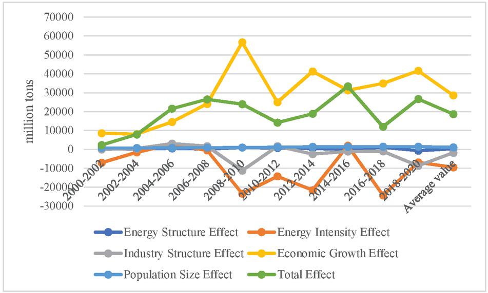
Figure 1 Factor decomposition of carbon emission changes from 2000 to 2020 (amount of contribution).
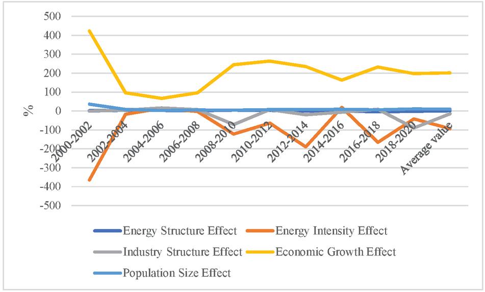
Figure 2 Factor decomposition of carbon emission changes from 2000 to 2020 (contribution rate).
From Figures 1–2, the energy structure effect contributes the most carbon emissions in 2008–2010; the energy intensity effect contributes the most negative carbon emissions in 2016–2018; the industrial structure effect contributes the most negative carbon emissions in 2008–2010; the economic output level effect contributes the most carbon emissions in 2018–2020; the population size effect in 2014–2016 contribute the most carbon emissions. we can see that the power shape impact is terrible in man or woman years and effective in the relaxation of the years; the strength depth impact contributes negatively to carbon emissions; the industrial shape impact has each effective and poor effects; the financial output degree impact and the populace measurement impact are positive.
3.2 Specific Breakdown of Each Factor
(1) Economic growth effect
From 2000 to 2020, the cost delivered of primary, secondary, and tertiary industries multiplied from 120.21 billion, 286.78 billion, and 206.42 billion RMB to 621 billion, 332.74 billion, and 425.91 billion RMB, respectively. Figure 3 suggests the contribution of monetary increase to carbon emissions of three industrial sectors each and every 4 years. 2000–2020, the contribution of the brought fee of primary, secondary, and tertiary industries to carbon emissions are 260 million t, 11.75 billion t, and 2.50 billion t CO respectively, which is equal to 0.51 million t, 3.86 million t, and 0.62 million t of carbon emissions for each 10,000 yuan expand in the brought fee of primary, secondary and tertiary industries respectively. China is nonetheless in the stage of shut correlation between monetary improvement and carbon emissions, and the percentage of energy-consuming industries in the enterprise is nonetheless high, and industrial development extensively drives the boom of carbon emissions, which is excluded from the developed nations that have carried out vulnerable correlation or decoupling between financial increase and carbon emissions.

Figure 3 Contribution of economic growth in the industrial sector to the change in carbon emissions.
(2) Energy intensity effect
Energy depth is one of the essential elements affecting carbon emissions. With the enchantment of science and technology, energy-saving technological know-how and gear have been popularized in China, and the administration of technique and system has been striving to “eat all the energy”, and the power consumption per unit of GDP has been reduced. The power depth of primary, secondary, and tertiary industries will minimize from 0.3, 2.5, and 0.5 t of preferred coal per 10,000 Yuan in 2000 to 0.1, 0.6, and 0.1 t of trendy coal per 10,000 Yuan in 2020. Figure 4 indicates the contribution of power depth to carbon emission modifications in the three industrial sectors, all displaying terrible effects. from 2000 to 2020, the strength depth decreased in primary, secondary, and tertiary industries making contributions 0.6 billion t, 6.07 billion t, and 1.26 billion t CO, respectively, which is equal to a discount in power depth of primary, secondary, and tertiary industries for every 1 t of preferred coal/10000 yuan, which can minimize three billion t, 3.2 billion t, and 3.14 billion t CO. From this, it is clear that the discount of electricity depth of the 2nd enterprise leads to the hugest carbon discount effect. Vigorous improvement of industrial power saving and consumption discounts and non-stop optimization of industrial shape are essential measures to limit carbon emissions.
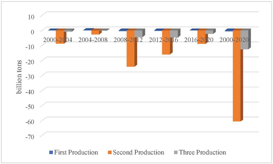
Figure 4 Contribution of energy intensity of industrial sectors to the change in carbon emissions.
(3) Industrial structure effect
By vigorously creating tertiary industries such as commerce and carrier industries with low strength consumption and low emission, and optimizing and adjusting secondary industries with excessive electricity consumption and excessive emission, China’s industrial shape has changed significantly, with the percentage of delivered fee of primary, secondary and tertiary industries in GDP altering from 19%, 47% and 34% in 2000 to 8%, 40% and 52% in 2020. The share of principal enterprise decreases significantly, the share of secondary enterprise decreases slightly, and the share of tertiary enterprise will increase significantly. Table 1 suggests the contribution of the share of three industrial sectors to the exchange of carbon emissions. 2000–2020, the contribution of industrial shape to the trade of carbon emissions is 100 million t, 930 million t, and 360 million t of carbon emissions, respectively. The poor impact of carbon emissions is most widespread in the secondary industry, and the tertiary industry, due to its quicker development, indicates a contribution to the increase of carbon emissions, however with a smaller impact. Overall, the enchantment of industrial shape has an increasing number of robust offsetting impacts on carbon emissions and is one of the essential instructions for carbon discounts in the future.
Table 1 Contribution of the structure of the industrial sector to the change in carbon emissions
| Year | First Production | Second Production | Three Production |
| 2000–2004 | -0.1 | -0.5 | 0.5 |
| 2004–2008 | -0.2 | 1.6 | 0.3 |
| 2008–2012 | -0.4 | -0.7 | 0.4 |
| 2012–2016 | -0.2 | -8.6 | 2.3 |
| 2016–2020 | -0.1 | -1.1 | 0.1 |
| 2000–2020 | -1.0 | -9.3 | 3.6 |
(4) Energy structure effect
The switch of high-carbon strength sources such as coal, oil, and herbal fuel to zero-carbon strength sources such as water and surroundings and the increasing cleanliness of power shape are the predominant methods to decrease carbon emissions. From 2000 to 2020, the percentage of fossil strength consumption in China declined from 93.9% to 86.2%, and the share of fossil power consumption in the primary, secondary, tertiary, and residential sectors all confirmed a lowering trend, whilst the share of smooth strength consumption with electrical energy as the service increased. In the thirteenth Five-Year Plan, all three industrial sectors and the residential region exhibit carbon emission offsetting effects.
Figure 5 shows the contribution of the fossil energy structure of the three industrial sectors and the residential sector to the change in carbon emissions. Overall, the contribution of the energy structure of primary, secondary, tertiary, and residential sectors to the change of carbon emission is 4.09 million t, 449.35 million t, 98.6 million t, and 33.76 million t CO, respectively, totaling 570 million t CO, and the effect of cleaner energy structure on carbon reduction is becoming more and more significant.
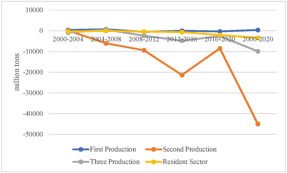
Figure 5 Contribution of the energy mix to changes in carbon emissions.
(5) Residential energy price, per capita income, and population size effects
The contributions of residential electricity prices, per capita profits, and populace measurement to carbon emissions in the residential region are proven in Table 2 residential area strength expenses measure the quantity of strength bought per unit of income. An enlarge in electricity costs implies that electricity spreading and wastefulness are curbed, decreasing residential carbon emissions. Thus, power fees substantially inhibit the boom in electricity consumption. 2000–2020, the quantity of electricity bought per 10,000 yuan in China decreases from 0.45 t of preferred coal to 0.11 t of well-known coal, which is equal to a 68,700 yuan make bigger in the value of every 1 t of general coal bump off by way of residents, with a full-size carbon emission reduction impact and a strong rate impact of 380 million t of CO.
Table 2 Carbon emission decomposition of the residential sector
| Year | Energy Price Effect | Income Effect | Population Effect |
| 2000–2004 | -1.1 | 0.6 | 0.2 |
| 2004–2008 | -0.4 | 1.4 | 0.1 |
| 2008–2012 | -1.1 | 2.3 | 0.1 |
| 2012–2016 | -0.7 | 2.1 | 0.1 |
| 2016–2020 | -0.5 | 0.7 | 0.1 |
| 2000–2020 | -3.8 | 7.1 | 0.6 |
Disposable income per capita is the most important driver of carbon emissions growth in the residential sector. With the growth of residents’ income, energy services such as household lighting, heating, and cooking drive the carbon emissions of the residential sector to increase. Disposable income per capita has an “amplifier” effect. From 2000 to 2020, every $1 increase in annual disposable income per capita drives an increase of 27,000 t of carbon emissions from residential energy consumption, and the per capita income effect increases by 710 million t of CO.
Population growth also has a certain degree of driving effect on the growth of residential energy consumption. 2000–2020, the increase in population drives residential consumption to increase by 0.6 billion t CO.
4 Carbon Emission Projection Based on the STIRPAT Model
4.1 STIRPAT Model
The IPAT mannequin was once formally proposed with the aid of Ehrlich P et al. [17] in 1972, and it is expressed as.
| (15) |
Where: I denotes environmental pressure; P denotes population; A denotes affluence; and T denotes socio-technical level.
This model has a simple structure, but it is more widely used in the study of environmental impact factors. And because the IPAT model treats the relationship between environmental impacts and each driver as simply a linear relationship of the same proportion, it cannot reflect the degree of change in environmental impacts when the drivers change.
Based on the IPAT model, Dietz T et al. [18] proposed the STIRPAT model to analyze the pressure generated by human factors on the environment, transforming the IPAT model into a stochastic form that takes into account the impact of separate changes in population, affluence, and technological factors on the environment, which is expressed as follows:
| (16) |
where: is the constant term; is the residual term; , , and are the index terms of population, affluence, and socio-technical level, respectively, which are also generally referred to as elasticity coefficients. When , the STIRPAT model will be reduced to the IPAT model, when , , and the larger, it means the greater the degree of influence on .
The STIRPAT model can be extended in practical applications to a variety of factors that have a significant impact on environmental change, such as the level of technology, energy consumption and energy industry structure, and can maintain the superior performance of the STIRPAT model as a whole. Therefore, the STIRPAT model is widely used to study the relationship between carbon emissions and various environmental influences.
The STIRPAT mannequin is a multivariate nonlinear equation, and in order to facilitate the use of software programs to estimate the exponents in it [19] and to get to the bottom of its heteroskedasticity, the two sides of the equation are generally converted into a linear model by taking the logarithm of the equation and obtaining the following form:
| (17) |
In order to find out about the influencing elements of carbon emissions of electricity consumption in an eastern province, the model (17) is extended with the actual situation of an eastern province, and the following model is constructed:
| (18) |
Where: is the carbon emission from energy consumption in an eastern province (MtC); P is the population (10,000 people); A is the affluence, expressed as GDP per capita (Yuan/person); T is the energy intensity, i.e., the ratio of energy consumption to GDP (tons of standard coal/10,000 yuan); J is the urbanization rate; N is the energy structure; is the elasticity coefficient, indicating that when each 1% change in P, A, T, J, and N, respectively causes change in I.
4.2 Ridge Regression Analysis
The STIRPAT mannequin was once first analyzed with the usage of the couple of linear regression algorithms encapsulated in SPSS software, and with variance inflation issue (VIF) used to be chosen as the comparison criterion [20], and the regression effects are proven in Table 3, in accordance to which the willpower coefficient of the STIRPAT mannequin used to be got as 0.99, which has a correct becoming effect, indicating that the accuracy of the geared up curve of complete carbon emissions can attain 9%. However, the VIFs of the STIRPAT mannequin are all & get; 10, and there is a hassle of multicollinearity amongst the influencing factors, which leads to distortion in the estimation of the STIRPAT mannequin or makes it hard to estimate accurately.
Subsequently, in order to do away with the trouble of multicollinearity amongst the influencing factors, this paper proposes a ridge regression approach to analyze the STIRPAT mannequin by calling the ridge regression process in the SPSS software program [21], in which the values of the ridge regression penalty time period K are from 0 to 1, and the step dimension is 0.01, with a complete of a hundred and one ridge parameter values; is chosen as the comparison criterion. The ensuing ridge hint plot is proven in Figure 6.
Table 3 Multiple linear regression results
| Non-standardized | Covariance | |||||
| Coefficient | Statistic | |||||
| Regression | Standard | Standardization | ||||
| Parameter | Coefficient | Error | Coefficient | Significance | Tolerance | VIF |
| Constant Term | 0.643 | 4.214 | — | 0.821 | 0.014 | 81.236 |
| lnP | 0.648 | 0.421 | 0.124 | 0.187 | 0.006 | 63.214 |
| lnA | 1.174 | 0.103 | 2.314 | 0 | 0.006 | 293.113 |
| lnT | 1.324 | 0.094 | 1.324 | 0 | 0.015 | 64.328 |
| lnJ | 0.014 | 0.463 | 0.009 | 0.934 | 0.096 | 194.761 |
| lnN | 0.712 | 0.104 | 0.324 | 0 | 0.063 | 9.967 |
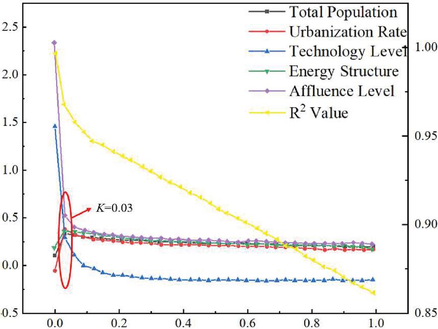
Figure 6 Ridge trace map.
From Figure 6, it can be viewed that in the ridge regression training, as the K cost increases, the exchange of every has an effect on the issue regularly stabilizes, however, the fee progressively decreases, so it is fundamental to choose the minimal K cost when is the most and every impact thing stabilizes, so as to gain the affect thing parameters with right magnitude at the minimal sacrifice of accuracy. When , the coefficients of the STIRPAT mannequin grow to be stable, and the most is 0.969. This suggests that the shape of ridge regression coaching is finest at , and the accuracy of the equipped curve of complete carbon emission can attain 96.9%. In different words, the becoming accuracy is excessive and meets the becoming necessities of the regression equation.
The ridge regression penalty term parameter was set to in SPSS software to train the STIRPAT model details, such as regression coefficients and standard errors, as shown in Table 4.
Table 4 Coefficients of STIRPAT model variables at
| Regression | Standard | Standard | ||
| Parameter | Coefficient | Error | Coefficient | Significance |
| Constant Term | 16.978 | 4.315 | — | 0.002 |
| lnP | 1.705 | 0.631 | 0.312 | 0.001 |
| lnA | 0.273 | 0.048 | 0.569 | 0 |
| lnT | 0.276 | 0.116 | 0.283 | 0.011 |
| lnJ | 1.176 | 0.269 | 0.317 | 0 |
| lnN | 1.720 | 0.324 | 0.297 | 0 |
It can be viewed that in accordance with the regression coefficients of every influencing factor, the regression coefficients of the 5 influencing elements of the complete population, affluence, urbanization rate, strength shape, and technological know-how stage are all positive, indicating a widespread high quality affect the relationship on whole carbon emissions, and the large the regression coefficient, the improved the impact [22]. It can be considered that strength shape has the best influence on carbon emissions, observed through the complete population, urbanization charge, and science level, and affluence has the least effect on carbon emissions; and all five influencing factors pass the significance test (), eliminating the problem of cointegration that exists when training the STIRPAT model by linear regression. According to the ridge regression results, it can be concluded that the constant term lna in the STIRPAT model is 16.978, and the regression coefficients of total population (P), affluence (A), technology level (T), urbanization rate (J) and energy structure (N) are 1.705, 0.273, 0.276, 1.176 and 1.72, respectively. In order to avoid the non-solution of the STIRPAT model, the STIRPAT model is constructed by setting the random error term lne=0. Thus, the STRPAT model is obtained as follows
| (19) |
The exponential transformation of Equation (4.2) leads to the STRPAT model that satisfies the accuracy requirement, i.e.
| (20) |
4.3 Historical Data Fitting
In order to ensure that the STIRPAT model can achieve the expected effect, the historical data of each influencing factor from 2000 to 2020 were substituted into the STRPAT model to calculate the predicted value of carbon emission from 2000 to 2020, and then compared with the real value of carbon emission from 2000 to 2020 to verify the validity of the proposed STIRPAT model, and the results are shown in Figure 7.
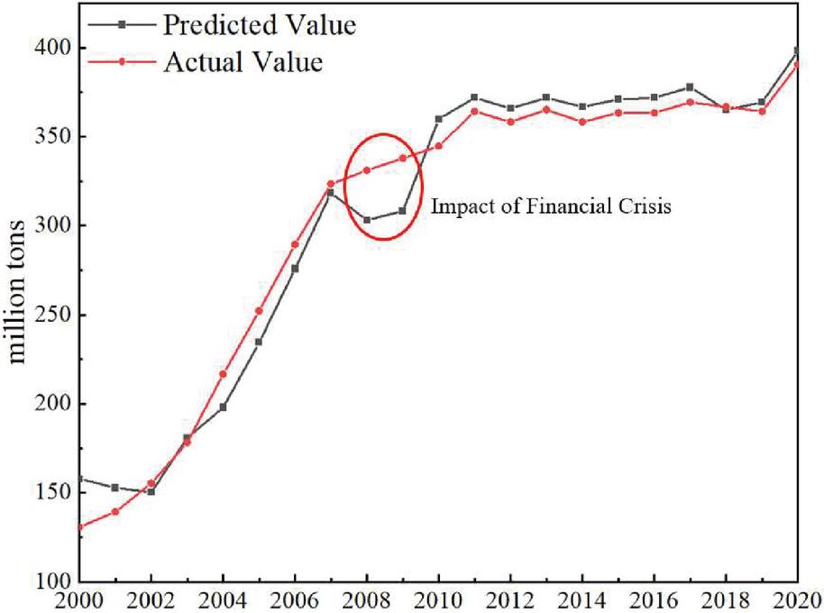
Figure 7 Comparison of predicted and true values of carbon emissions from the STIRPAT model.
As can be viewed from Figure 7, the STIRPAT mannequin proposed in this paper has an excellent standard fit, and the root suggests rectangular error between the expected and proper values of carbon emissions is 6.1%. The STIRPAT mannequin can meet the accuracy necessities and can be used to predict the future carbon emissions of the region. In 2008 and 2009, due to the impact of the financial crisis, the proportion of fossil energy consumption and energy consumption intensity in the region decreased to a certain extent, resulting in a slowdown in the growth rate of actual carbon emissions in that year. However, due to the abnormal proportion of fossil energy consumption and energy consumption intensity, the prediction values calculated by the STIRPAT model in this paper show a downward trend compared with 2007, which makes the prediction error of 2008 and 2009 large. Due to the uncertainty of future scenarios, a state of affairs comparable to the monetary disaster in 2008 can also have an effect on the prediction of future carbon emissions. In order to greater precisely analyze the improvement of future carbon emission developments and decrease the effect of uncertainty of future scenarios, this paper chooses the state of affairs evaluation approach mixed with the STIRPAT mannequin to predict the future carbon emissions in the region.
4.4 Analysis of Scenario Setting
Scenario evaluation is a qualitative forecasting approach that assumes the continuation of modern insurance policies and improvement stipulations into the future and develops an evaluation of the lookup object. It has the benefits of environmental analysis, choice making, enhancing the adaptability of STRPAT mannequin, and optimizing aid allocation, and is generally utilized in sustainable improvement lookup and monetary and environmental improvement forecasting. In this paper, three eventualities of high-speed development, baseline improvement, and low-carbon improvement are set for every influencing factor. By combining specific improvement situations of every influencing factor, 9 unique improvement situations are obtained, as proven in Table 5.
Table 5 Scenario combinations
| Scenario | Energy Structure | Urbanization Rate | Total Population | Affluence Level | Energy Intensity |
| 1 | High-speed | Low-carbon | Low-carbon | Low-carbon | High-speed |
| 2 | High-speed | Baseline | High-speed | High-speed | High-speed |
| 3 | Baseline | Baseline | Baseline | Baseline | Baseline |
| 4 | Baseline | High-speed | High-speed | Baseline | Baseline |
| 5 | Low-carbon | Low-carbon | Low-carbon | Low-carbon | Low-carbon |
| 6 | Low-carbon | Baseline | Low-carbon | Baseline | Low-carbon |
| 7 | Low-carbon | Baseline | Baseline | Low-carbon | Baseline |
| 8 | Low-carbon | High-speed | Baseline | High-speed | Low-carbon |
| 9 | Low-carbon | High-speed | High-speed | High-speed | Low-carbon |
In this paper, we take 2020 as the base year, and set the parameters of future strength structure, electricity intensity, monetary development, populace and urbanization charge beneath specific eventualities based totally on the LMDI decomposition effects in part 3.2 and applicable insurance policies such as the 14th Five-Year Plan and the 2035 visionary desires of the region: (1) In the base scenario, the fee of exchange of every influencing aspect is primarily based on the corresponding price of trade of every influencing factor; (2) beneath the high-speed improvement scenario, the proportion of fossil electricity consumption in the power shape decreases slowly, the strength depth is higher, and the regional monetary and populace increase hastens in contrast to the baseline scenario; (3) underneath the low carbon improvement scenario, the share of fossil electricity consumption decreases faster, the strength depth is lower, and the regional financial and populace increase slows down in contrast to the baseline scenario. increase charge slows down.
Based on the constructed STIRPAT model framework for carbon emission projections for different combinations of scenarios in Table 5, the obtained results are shown in Figure 8, and their peak times and peak sizes for different scenarios are shown in Table 6.
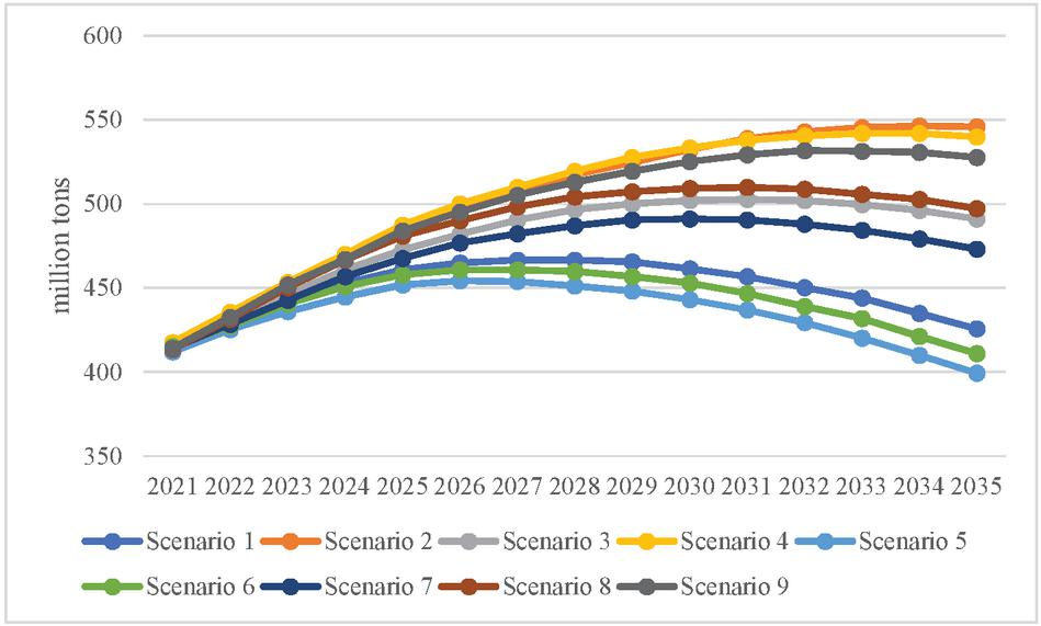
Figure 8 Comparison of carbon emissions in the region under multiple scenarios.
As seen in Figure 8 and Table 6, only Scenario 2 of the nine scenario combinations does not peak by 2035. Among the remaining 8 scenarios, 4 scenarios, namely Scenario 1, Scenario 5, Scenario 6, and Scenario 7, can achieve the carbon peak target by 2030. Therefore, these four scenarios were selected for analysis.
Table 6 Predicted results of carbon bloom in the region under 9 combinations of scenarios
| Scenario | Year of Peak Carbon Emission | Peak Carbon Emission |
| 1 | 2027 | 471.34 |
| 2 | Not Peaking | — |
| 3 | 2031 | 501.26 |
| 4 | 2034 | 561.78 |
| 5 | 2026 | 431.95 |
| 6 | 2027 | 458.78 |
| 7 | 2030 | 497.63 |
| 8 | 2031 | 513.65 |
| 9 | 2034 | 536.91 |
From the trends of the four scenarios in Figure 8, we can get that although CO peaks around 2030 in Scenario 7 and completes the time target, the carbon emission per unit GDP is still too high at this time, which does not meet the carbon emission standards of the 14th Five-Year Plan and 2035 Vision for the region, and the carbon emission decreases slowly after peaking, so it is difficult to reach the carbon neutral target in 2060. Scenario 1 and Scenario 6, on the other hand, are expected to achieve the carbon neutrality target by 2060 because of the declining population growth rate and the rapid reduction of carbon emissions after reaching the peak. Scenario 6 has a higher level of technology compared to Scenario 1, which accelerates the transformation of energy structure and decreases energy intensity faster, and can significantly reduce carbon emissions, although it does not advance the time to peak. In Scenario 5, since the urbanization rate and per capita GDP growth rate are lower than those in Scenario 6, the carbon peak time can be advanced to about 2026, and the corresponding carbon emission peak is the smallest, which can also maintain the rapid decline of carbon emissions after the peak and achieve the carbon neutral target by 2060.
Based on the analysis of carbon emission prediction results, the following suggestions are put forward for emission reduction:
(1) On the energy supply side, optimize the energy structure and promote the transformation of clean energy and electrification. In the rising stage before carbon peaking, the allocation and regulation capacity of the power system should be enhanced, and infrastructure construction such as natural gas, wind and photovoltaics, nuclear power and hydropower should be increased. In the stage of emission reduction and neutrality after carbon peaking, the energy supply side should get rid of the use of coal energy, meet new energy demand through low-carbon fuels and new energy, and provide support for the energy system to achieve zero carbon.
(2) On the energy consumption side, focus on energy conservation and carbon reduction, and maximize energy utilization guided by technological innovation. Promote the efficient transformation of energy consumption in energy-consuming sectors such as industry, buildings, and transportation, eliminate backward production capacity, optimize production structure, promote low-carbon industrial production, and guide energy-consuming sectors to transform from “energy reduction” to “energy saving”.
Table 7 Correlation coefficients of energy consumption and GHG emission indicators with climate change indicators
| Energy Consumption Indicator | |||||
| Total | |||||
| Total | Industrial | ||||
| Energy | Energy | Electricity | CO | ||
| City Climate | Climate Indicator | Consumption | Consumption | Consumption | Emission |
| Temperature Variation | Average City Temperature | 0.82 | 0.81 | 0.76 | 0.71 |
| Average Suburb Temperature | 0.57 | 0.56 | 0.54 | 0.52 | |
| Temperature Difference | 0.91 | 0.93 | 0.92 | 0.76 |
5 Coercion of Energy Consumption Processes to Climate Change
5.1 Correlation Analysis of Energy Consumption, Its CO Emission-related Indicators, and Climate Change
Based on the above evaluation of CO estimation of electricity consumption in an jap province from 2000 to 2020 and end-use strength consumption from 2021 to 2035, the correlation coefficients of complete strength consumption, complete electrical energy consumption, industrial electricity consumption, and CO emissions from end-use strength consumption have been chosen to analyze the correlation coefficients with applicable local weather indications such as nearby temperature trade and humidity exchange in an jap province [23]. As proven in Table 7, the correlation coefficients of power consumption warning signs and temperature exchange indications all skip the importance take a look at the P 0.01 level, with the best possible correlation coefficient with the suburban temperature difference, which are larger than 0.9 and omit the magnitude take a look at the P 0.001 level, which suggests that there is a pretty considerable impact of greenhouse gasoline emissions from strength consumption in an eastern province on the city warmness island impact [24]; among them, the correlation coefficient between total industrial energy consumption and peri-urban temperature difference is slightly higher than that of total energy consumption and electricity consumption, indicating that industrial energy consumption in an eastern province during the whole period of 20002020 is the main factor leading to the temperature difference between urban and suburban areas, and the reason is mainly because the energy consumption structure of a province in the east is dominated by industry, and the greenhouse gas emissions brought by the energy consumption process mainly come from the industrial sector. However, it should be pointed out that according to the above CO emission analysis of different industrial sectors in 20212035, since 2000, due to the rapid acceleration of urban construction in a province in the east, the accelerated development of the tertiary industry, especially the development of the transportation industry, and the improvement of urban living standards. As a result, the energy consumption demand of the construction, transportation, warehousing and postal industry, wholesale, retail industry, accommodation, catering industry and living consumption sector is growing rapidly. The ensuing expansion in CO emissions has been the major reason for city warming and warmness island impact in an eastern province when you consider that it entered a length of speedy urbanization.
As with the energy consumption indicator, the correlation between total end-use energy CO emissions and temperature change is higher than that of humidity change, with the highest correlation coefficient of 0.76 with the suburban temperature difference, and passing the significance test at the P 0.01 level, further confirming that CO emissions from the energy consumption process are the main cause of the heat island effect; due to the small sample data of end-use energy CO emissions, the correlation coefficient is lower than that of the energy consumption indicator. Therefore, the correlation coefficient is lower than that of energy consumption indicators.
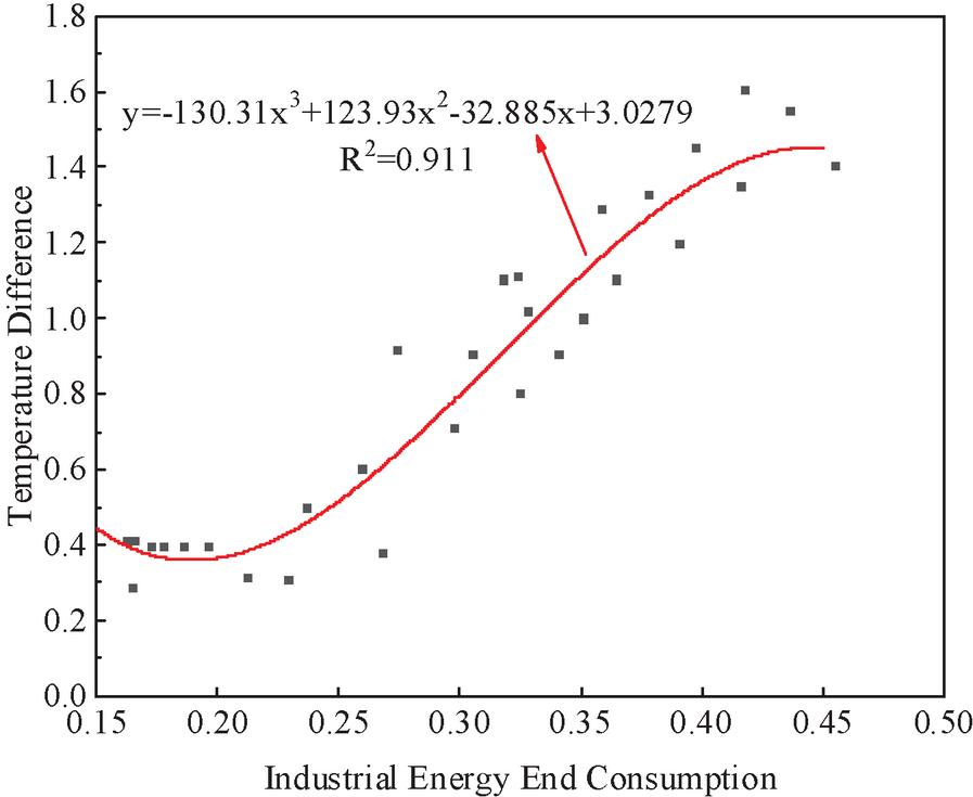
Figure 9 Relationship between industrial energy end-use consumption and suburban temperature difference from 2000 to 2020.
5.2 Coercive Modeling of Energy Consumption on Climate Change
Based on the analysis of correlation coefficients among the indicators above, the indicators with high correlation coefficients were selected to further analyze the model of the coercive relationship between energy consumption and local climate change [25]. The correlation coefficient analysis showed that industrial energy consumption had the highest impact on peri-urban temperature difference, and considering the completeness of the sample data [26], the coercive model of energy consumption on peri-urban temperature difference was analyzed with industrial energy end-use consumption from 2000 to 2020 as the independent variable and peri-urban temperature difference as the response variable, and the regression analysis showed that the fitted equations of both were.
| (21) |
As shown in Figure 9, the relationship between the increase in industrial energy end consumption and the suburban temperature difference is consistent with a cubic polynomial curve growth, the overall peri-urban temperature difference increases with the increase in industrial energy end-use consumption, mainly because the increase in energy consumption leads to an increase in CO, which in turn leads to an increase in peri-urban temperature difference due to the greenhouse effect. Specifically, from 2000 to 2010, before the industrial energy terminal consumption of 2.3 10 kg of standard coal, the change in the suburban temperature difference was small and basically maintained at 0.4C; since 2010, the relationship has been maintained close to linear, and the coercive effect of the increase in energy consumption on the suburban temperature difference is significant; since 2013, the curve growth starts to level off.
The correlation analysis of energy consumption indicators and temperature change indicators shows that greenhouse gas emissions from energy consumption have a highly significant effect on the urban heat island effect; the correlation coefficients of total industrial energy consumption and suburban temperature difference among energy consumption indicators are slightly higher than those of total energy consumption and electricity consumption; the coercive relationship between the increase of industrial energy consumption and the suburban temperature difference is consistent with a cubic polynomial curve growth; the rapid development of the tertiary industry since 2000 and the resulting increase in CO emissions are the main causes of temperature increase and heat island effect in urban areas.
6 Conclusion
This paper adopts the LMDI decomposition technique to quantitatively analyze the elements of carbon emission adjustments in industrial and residential sectors in an eastern province of China and uses the STIRPAT prediction model to set nine different development scenarios to forecast the total carbon emissions until 2035, and the conclusions are as follows.
(a) The LMDI decomposition consequences exhibit that from 2000 to 2020, amongst carbon emissions of three industrial sectors, monetary increase indicates a massive fantastic effect, whilst electricity intensity, industrial shape, and strength shape have terrible effects, with contribution fees of 228.9%, 116.7%, 8.9% and 8.4%, respectively, and the optimization of industrial shape and easy electricity shape play a more and more giant role. In the residential sector, electricity shape and electricity charge have terrible results on carbon emissions, with contribution costs of 0.5% and 5.9%, respectively; per capita profits and populace dimension have high-quality results on carbon emissions, with contribution fees of 10.1% and 0.6%, respectively.
(b) The results of nine scenarios show that with low-carbon development as the core in 2021–2035 and appropriate adjustment of development strategies, the region is expected to achieve carbon peaking in 2026–2030. The comparison analysis shows that keeping the urbanization rate and economic level growth rate unchanged, reducing the population growth rate, and accelerating energy restructuring and emission reduction technology development are the optimal emission reduction planning paths in the region. Under this scenario, the region is able to maintain a high rate of economic and urbanization development while having a good ability to reduce emissions. The projection results show that the region will reach the carbon peak in 2027, after which carbon emissions will keep declining at a high rate, and is expected to achieve carbon neutrality by 2060.
(c) The correlation coefficients of energy consumption indicators and temperature change indicators all pass the significance test at the P 0.01 level, among which the correlation coefficients with temperature difference are the highest, all of which are greater than 0.9 and pass the significance test at the P 0.001 level; among the energy consumption indicators, the correlation coefficients of total industrial energy consumption and temperature difference are slightly higher than those of total energy consumption and electricity consumption; the coercive relationship between the increase of energy consumption and the temperature difference is in accordance with the third polynomial curve growth.
Many scholars have analyzed the influencing factors of environmental stress in different regions, but studies from a micro perspective such as at the city and district level are more lacking, ignoring the possible intra-regional variability. In addition, the drivers of environmental stress are different for different research subjects, and the respective influencing factors need to be refined. Therefore, when analyzing regional environmental stress, refining and decomposing the influence of each variable from a microscopic perspective will be a direction for future research.
References
[1] Le Quéré C, Takahashi T, Buitenhuis E T, et al. Impact of climate change and variability on the global oceanic sink of CO[J]. Global Biogeochemical Cycles, 2010, 24(4).
[2] Breecker D O, Sharp Z D, McFadden L D. Atmospheric CO concentrations during ancient greenhouse climates were similar to those predicted for AD 2100[J]. Proceedings of the National Academy of Sciences, 2010, 107(2): 576–580.
[3] Zhu Changzheng, Yang Sha, Liu Pengbo, et al. Carbon peak time prediction in China’s transportation industry[J]. Transportation Systems Engineering and Information, 2022, 22(6): 291.
[4] Kang H, Gao J, Hui G. Laboratory Evaluation of CO Flooding: A Strategic Technology for Sustainable Development of Oil Companies[J]. Strategic Planning for Energy and the Environment, 2023: 21–36.
[5] Qu JF, Chu CHL, Ju MT, et al. Decomposition of carbon emission drivers of residential energy consumption–Tianjin city as an example[J]. Ecological Economy, 2017, 33(4): 38–42.
[6] Guo Y, Zhao M. Research on sustainable energy development from the perspective of focusing on carbon peaking and neutrality[J]. Strategic Planning for Energy and the Environment, 2022: 345–362.
[7] Xie Di, Tian Yinglin, Wang Guangqian, et al. Research on carbon neutral pathways in Qinghai Province[J]. Journal of Applied Basic and Engineering Sciences, 2022.
[8] Sebos I, Progiou A G, Kallinikos L. Methodological framework for the quantification of GHG emission reductions from climate change mitigation actions[J]. Strategic planning for energy and the environment, 2020: 219–242.
[9] Yang P, Liang X, Drohan P J. Using Kaya and LMDI models to analyze carbon emissions from the energy consumption in China[J]. Environmental Science and Pollution Research, 2020, 27: 26495–26501.
[10] Ang B W. Decomposition analysis for policymaking in energy:: which is the preferred method?[J]. Energy policy, 2004, 32(9): 1131–1139.
[11] Chen Junhua, Li Qiaochu. Study on the factors influencing carbon emissions of energy consumption in Sichuan Province in the context of the construction of Chengdu-Chongqing twin-city economic circle–based on LMDI model perspective [J].
[12] Kim H S, Noulèkoun F, Noh N J, et al. Future Projection of CO Absorption and N2O Emissions of the South Korean Forests under Climate Change Scenarios: Toward Net-Zero CO Emissions by 2050 and Beyond[J]. Forests, 2022, 13(7): 1076.
[13] Fu B, Gasser T, Li B, et al. Short-lived climate forcers have long-term climate impacts via the carbon–climate feedback[J]. Nature Climate Change, 2020, 10(9): 851–855.
[14] Friedlingstein P, Bopp L, Ciais P, et al. Positive feedback between future climate change and the carbon cycle[J]. Geophysical Research Letters, 2001, 28(8): 1543–1546.
[15] Dahlmann K, Grewe V, Matthes S, et al. Climate assessment of single flights: Deduction of route specific equivalent CO emissions[J]. International Journal of Sustainable Transportation, 2023, 17(1): 29–40.
[16] Bae J H. Impacts of income inequality on CO emission under different climate change mitigation policies[J]. Korean Econ Rev, 2018, 34(2): 187–211.
[17] Ehrlich P, Holdren J. Impact of population growth[J]. Population, resources, and the environment, 1972, 3: 365–377.
[18] Dietz T, Rosa E A. Rethinking the environmental impacts of population, affluence and technology[J]. Human ecology review, 1994, 1(2): 277–300.
[19] Pan Yue, Zhu Jiye, Ye Yi’an. Analysis of carbon emission impact drivers in Jiangsu Province based on STIRPAT model[J]. Environmental Pollution and Prevention, 2014, 36(12): 104–109.
[20] Huang Rui, Wang Zheng, Ding Guanqun, et al. Analysis and trend prediction of carbon emissions from energy consumption in Jiangsu Province based on STIRPAT model[J]. Geography Research, 2016, 35(4): 781–789.
[21] Martin Calvo M, Prentice I C. Effects of fire and CO 2 on biogeography and primary production in glacial and modern climates[J]. New Phytologist, 2015, 208(3): 987–994.
[22] JI Xing-Quan, ZHAO Guo-Hang, YU Yi-Xiao, et al. Carbon emission factor decomposition and peak prediction method based on 4E balance[J]. High Voltage Technology, 2022.
[23] Torvanger A, Grimstad A A, Lindeberg E, et al. Quality of geological CO storage to avoid jeopardizing climate targets[J]. Climatic change, 2012, 114: 245–260.
[24] Roy T, Bopp L, Gehlen M, et al. Regional impacts of climate change and atmospheric CO on future ocean carbon uptake: A multimodel linear feedback analysis[J]. Journal of Climate, 2011, 24(9): 2300–2318.
[25] Wang Yuan, Zhao Li-Man, Yu Xia, et al. Evaluation of carbon emission changes of energy consumption and local climate change stress in Shanghai[J]. Journal of Fudan: Natural Sciences Edition, 2015 (4): 439–448.
[26] Yao Y, Li G, Lu Y, et al. Modelling the impact of climate change and tillage practices on soil CO emissions from dry farmland in the Loess Plateau of China[J]. Ecological Modelling, 2023, 478: 110276.
Biographies

Kunyue Zhang received her Bachelor’s degree in Land Resource Management from China Agricultural University in 2017. Now she is studying for a master’s degree in Land Resource Management at China Agricultural University. Research areas and directions include territorial spatial planning, geographic information systems and environmental impact assessment.

Mingru Tao received his bachelor’s degree in Land Resource Management from China Agricultural University in 2017 and is now studying for a master’s degree in land Resource Management at China Agricultural University. Research fields and directions include territorial space planning, protection of cultivated land resources and food safety.

Jinmin Hao (1960–), male, born in Jinzhong, Shanxi Province, Doctor, professor. Her research interest covers territorial spatial planning, land evaluation, soil improvement and utilization, Regional governance and sustainable development.
Strategic Planning for Energy and the Environment, Vol. 43_1, 81–112.
doi: 10.13052/spee1048-5236.4314
© 2023 River Publishers