Low-Carbon Economic Dispatch of Integrated Energy Systems in Multi-Form Energy-intensive Parks Based on the ICT-GRU Prediction Model

Liaoyi Ning^*, Kai Liang, Bo Zhang, Yang Gao and Zhilin Xu

Anshan Power Supply Company of State Grid Liaoning Electric Power Co., Ltd, Anshan 114000, China
E-mail: NingLY_AS.163.com
*Corresponding Author

Received 26 June 2023; Accepted 11 August 2023; Publication 09 January 2024

Abstract

This paper presents a solution to the issues of redundancy and ambiguity in predicting variables associated with renewable energy output while aligning with the objectives of the “dual-carbon” energy strategy. A low-carbon economic dispatch method for multi-form energy-intensive parks is proposed, employing the ICT-GRU prediction model. Leveraging historical generation data, the ICT-GRU model enables accurate forecasting of renewable energy output. Subsequently, a comprehensive energy system model is developed considering the carbon emission characteristics and control features of park entities. The model aims to minimize operational costs and facilitate low-carbon economic dispatch. The effectiveness of the proposed method is demonstrated through a case study conducted in a multi-form energy-intensive load park integrated into a power grid. The results validate its capability to achieve low-carbon economic operation and provide valuable insights for grid dispatch optimization.

Keywords: ICT-GRU prediction, multi-form energy-intensive park, integrated energy system, low-carbon economic dispatch.

1 Introduction

In the context of the “dual carbon” energy strategy, the integration of new energy sources plays an increasingly vital role in the power system. According to the “Analysis and Forecast Report on the National Power Supply and Demand Situation for 2021–2022” published by the China Electricity Council [1], non-fossil fuel power generation capacity surpassed coal-fired power generation by the end of 2021, with a total installed capacity of 1.12 billion kilowatts. Notably, wind power capacity experienced year-on-year growth of 16.6% to reach 330 million kilowatts, while solar power capacity grew by 20.9% to reach 310 million kilowatts. However, the intermittent and uncertain nature of renewable energy generation poses challenges to the optimization and scheduling of microgrid loads [2]. Addressing the uncertainty associated with new energy sources becomes crucial for achieving a real-time balance between power supply and demand, particularly in the optimization and scheduling of microgrid loads [3].

To tackle these challenges, recent research efforts have focused on utilizing prediction methods to mitigate the uncertainties in renewable energy generation [4–8]. Incorporating prediction models into microgrid optimization and scheduling enhances accuracy and expands the applicability of these approaches. For example, reference [9] employed data mining techniques to analyze the fluctuation characteristics of photovoltaic output, leading to the development of a deep learning prediction model that effectively captures the nonlinear relationship between weather fluctuations and power variations. Similarly, [10] proposed a simulation method that comprehensively represents longitudinal and transverse characteristics, ensuring the consideration of output levels’ impact on the probability distribution of prediction errors and achieving improved horizontal autocorrelation. Furthermore, [11] addressed the uncertainty of wind power by developing a wind power prediction model with reduced errors, thereby enhancing the power grid’s capacity to accommodate wind energy. While these references have made notable contributions to renewable energy generation prediction, it remains essential to address the redundancy and ambiguity present in the variables required for accurate predictions.

The Integrated Energy System (IES) is recognized as a powerful technology for achieving the “dual carbon” goals by enhancing renewable energy absorption and reducing carbon emissions [12–15]. Previous studies have investigated the coordinated scheduling of the integrated energy system and active distribution network within parks, leading to improvements in renewable energy absorption, load curve optimization, and load fluctuation reduction [16]. Another study proposed a flexible and cost-effective dispatch strategy for the integrated energy system in parks, considering optimal output ranges and carbon trading, resulting in enhanced economic benefits [17]. Furthermore, researchers have explored source-load interactive scheduling strategies and the utilization of multiple complementary energy sources to reduce costs and increase the absorption of new energy in parks [18]. Despite these contributions, the analysis of carbon emission characteristics on both the source and load sides of parks remains limited, with most studies focusing on carbon emission operating costs on the supply side.

To address this research gap, it is crucial to consider the carbon emission characteristics on both the source and load sides of parks, as this will enable a more accurate assessment of the potential for adjusting and optimizing demand-side resources. Such an analysis will significantly improve the effectiveness and efficiency of integrated energy systems in achieving their low-carbon objectives.

In addition to carbon emission optimization, integrated energy systems in parks offer numerous advantages for optimizing energy consumption. Through coordinated scheduling and the utilization of various dispatch units, including renewable energy sources and gas-fired units, parks can optimize their energy consumption while reducing carbon emissions. This comprehensive approach takes into account both economic and environmental factors, resulting in improved economic benefits and a more sustainable energy landscape.

In conclusion, the development of prediction methods is crucial for addressing the uncertainty of renewable energy generation. Integrating and optimizing energy systems within parks plays a vital role in enhancing renewable energy absorption and contributing to carbon reduction objectives. By considering the carbon emission characteristics of both the source and load sides of parks, the full potential of demand-side resources can be harnessed, effectively supporting the achievement of the “dual carbon” objectives.

This paper presents a low-carbon economic dispatch method for the integrated energy system of a multi-form energy-intensive-consuming park, leveraging the ICT-GRU prediction model. By considering the carbon characteristics of entities on both the source and load sides, the proposed method aims to achieve low-carbon economic operation within the park. The effectiveness of the method is validated through a case study, providing valuable guidance for grid dispatch.

2 Renewable Energy Output Prediction Model Based on ICT-GRU

2.1 Obtaining Classification Labels for Renewable Energy Output Characteristics

In recent years, there has been a significant advancement in automation within power systems, accompanied by the development of data collection technologies. As a result, the extraction of load characteristics from vast amounts of data has become increasingly crucial. While renewable energy output is inherently uncertain, it also exhibits certain regularities in its generation patterns. In this study, we aim to investigate the characteristics of renewable energy output in a park by leveraging data mining techniques applied to historical generation data.

To achieve this objective, we employ an ensemble clustering technique within the data mining framework. This approach offers several advantages over traditional clustering methods, such as K-means and hierarchical clustering. One significant advantage is its ability to overcome the problem of the K-means algorithm getting trapped in local optima [19]. The ensemble clustering technique combines the strengths of various clustering methods, resulting in a more robust and accurate analysis. The step-by-step process of this technique is as follows:

Figure 1 The flow chart of integrated clustering technology.

The ensemble clustering technique utilizes the silhouette coefficient [20] to determine the optimal number of clusters, denoted as K. The silhouette coefficient is a metric used to assess the quality of clustering results. It is defined as follows:

$I_{SC}$	$={\displaystyle \frac{b(X_i)-a(X_i)}{\max \{a(X_i),b(X_i)\}}}$	(1)
$a(X_i)$	$={\displaystyle \frac{{\sum }_{X_i\in C_K}\mathrm{dist}(X_i,X_i^{\prime })}{|C_K-1|}}$	(2)
$b(X_i)$	$=\min {\displaystyle \frac{{\sum }_{X_i,\in C_1}\mathrm{dist}(X_i,X_i^{\prime })}{|C_1|}}$	(3)

The equation mentioned above defines the silhouette coefficient, where $N$ represents the number of samples, $a(X_i)$ denotes the average distance between $X_i$ and other objects within its cluster, and $b(X_i)$ represents the minimum average distance from Xi to all other clusters.

To determine the optimal number of clusters, we select the value of K that maximizes the silhouette coefficient. Subsequently, the obtained clustering results are utilized as classification labels to characterize the renewable energy generation characteristics in the park. Each renewable energy output curve is assigned a classification label from the set $V=\{1,2,\mathrm{\dots }K\}$ based on its respective category. These labels are then utilized as one-dimensional input variables for the prediction model.

2.2 Renewable Energy Output Prediction Model Based on ICT-GRU

The GRU (Gated Recurrent Unit) network, an enhanced variant derived from the LSTM (Long Short-Term Memory) network, presents notable advancements. By integrating the forget gate and input gate, the GRU network optimizes the three gate functions of LSTM, resulting in the creation of an update gate [21]. Moreover, it combines the neuron state and hidden state, effectively addressing the challenging issue of “vanishing gradients” that often arise in RNN networks. Consequently, the GRU network achieves a reduction in the parameter count of LSTM units, thereby shortening the training time of the model. Figure 2 illustrates the fundamental unit structure of the GRU network, while Equation (4) presents its mathematical description.

$$\{\begin{array}{c}{r}_t=\delta (W_t{r}_t+U_r{h}_{t-1})\hfill \\ z_t=\delta (W_z{r}_t+U_z{h}_{t-1})\hfill \\ {\tilde{h}}_t=f(W_h{X}_t+W_h(r_t\mathrm{\Theta }{h}_{t-1}))\hfill \\ ht=z_t\mathrm{\Theta }{h}_t+(1-{\tilde{z}}_t)\mathrm{\Theta }{h}_{t-1}\hfill \end{array}$$

(4)

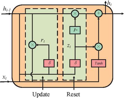
Figure 2 Basic unit of GRU network.

Equation (4) introduces various symbols to represent different variables and functions. $X_t$ stands for the input vector at time $t$, $h_{t-1}$ represents the state memory variable from the previous time step, $ht$ represents the state memory variable at time $t$, $r_t$ denotes the update gate state at time $t$, and $z_t$ signifies the reset gate state at time $t$. The sigmoid activation function is denoted as $\delta$, while the tanh activation function is represented by $f$. The weight matrices $W_r$, $U_r$, $W_z$, $U_z$, $W_h$, and $U_h$ correspond to the gates and candidate sets.

In the context of predicting renewable energy output, temporal factors such as season and month are influential. Table 1 displays the relevant time factors. Incorporating these time factors is important to improve prediction accuracy. This study aims to explore the generation characteristics of renewable energy using historical data. Instead of directly including the specific time variables, they are replaced by the classification labels obtained from the previous section, while still considering the time type $H_t$. This approach eliminates redundancy and ambiguity associated with the time factors. The combined classification labels $V$ and $H_t$ serve as input data for the GRU load prediction model, enabling the generation of accurate load prediction values. The GRU network structure employed in this study comprises three layers, as depicted in Figure 4. Figure 2 provides an overview of the basic flow of the approach.

Table 1 Basic time variables

Factor Type	Factor Description
$S_t$	Seasonal type, $S_t=1-4$
$M_t$	Month Type, $S_t=1-12$
$D_t$	Type of daily output days within the month, $D_t=1-31$
$W_t$	Week Type, $W_t=1-7$
$H_t$	Time type, $H_t=1-24$
$G_t$	Working Day Type, $G_t=1/0$
$J_t$	Types of festivals, $J_t=1/0$

Figure 3 delineates the predictive framework of ICT-GRU, a model that synergistically integrates conventional Information and Communication Technology (ICT), Euclidean distance-based AKmeans clustering, and Gated Recurrent Units (GRU) networks, thereby facilitating enhanced precision in load forecasting. Initially, using ICT tools, historical load data is extracted from grid sensors and subsequently undergoes essential preprocessing to ensure its reliability and consistency. This data is then subjected to AKmeans clustering predicated on Euclidean distance, highlighting analogous load patterns and consequently producing cluster labels denoted as V, effectively capturing the inherent structure and cyclical tendencies of the data. In the ensuing phase, the historical load values of each data point or timeframe are replaced with their respective cluster labels V, streamlining the data’s dimensionality and providing a structured input for GRU model training. Upon utilizing this transformed data, specifically the cluster label V, a GRU predictive model is constructed and calibrated through iterative refinement with optimization algorithms using the historical load data’s cluster labels. The culmination involves leveraging ICT tools for real-time acquisition of fresh load data, which, after undergoing cluster label substitution, is introduced to the pre-trained GRU model, yielding the final output as the predicted future load values.

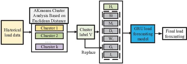
Figure 3 ICT-GRU forecasting process.

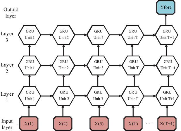
Figure 4 Three-layer GRU network structure.

Figure 4 illustrates the schematic of a three-tiered GRU network architecture established in this study. The model intakes historical load data and processes it through three sequential GRU layers to produce a final predicted load value. In essence, the architecture consists of three stacked GRU layers. The initial layer accepts and processes the historical load data, whose output serves not only as input for the subsequent GRU unit within the same layer but is also channeled to the second GRU layer. This pattern continues with the second GRU layer’s output feeding into the third GRU layer, which, upon further processing, directs its outcome through a fully connected layer to generate the predicted load value. Such a multilayered approach enhances the model’s capacity to discern intricate patterns and relationships from the input load data, leading to more accurate load predictions.

To assess the accuracy of the prediction method employed in this research, the Mean Square Deviation (MSD) ratio is utilized as an evaluation metric, which is a commonly adopted measure in grey forecasting theory. The MSD ratio allows for a comprehensive assessment of the prediction accuracy, providing valuable insights into the performance of the proposed method.

3 Low-carbon Economic Dispatch Model for Multi-modal High-capacity Energy Park Integrated Energy Systems

3.1 Composition of the Parking Structure

The park under consideration encompasses a diverse range of distributed energy sources, including wind power, photovoltaic systems, and micro gas turbines. In addition, it encompasses various types of loads, such as heat pumps, electric chillers, energy storage devices, conventional loads, and multi-mode energy-intensive loads. The multi-mode energy-intensive loads comprise discrete, continuous, and time-shifted loads with energy-intensive requirements. Furthermore, energy storage devices consist of battery energy storage systems, thermal storage tanks, and cold storage tanks. The energy flow diagram depicting the interconnected energy flows within the park is illustrated in Figure 5.

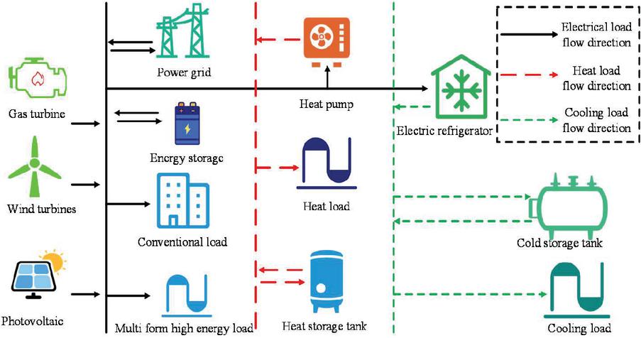
Figure 5 Schematic diagram of energy flow in multiform energy-intensive loading park.

3.2 Low-carbon Economic Dispatch Model

This study addresses the carbon emission characteristics and controls aspects of the entities within the park. The primary objective is to minimize the operating cost of a multi-form energy-intensive load park. To achieve this goal, a comprehensive low-carbon economic model for the park is formulated, incorporating multiple dispatch units. The specific details of the proposed model are presented below:

$$F=\min (C_{\mathit{gc}}+C_{\mathit{xn}}+C_{\mathit{cn}}+C_{\mathit{gt}}+C_{\mathit{ry}}+C_{\mathit{rp}})$$

(5)

$$\{\begin{array}{c}{C}_{\mathit{gc}}=C_c\sum _{t=1}^T(Q_{\mathit{sy}}{P}_{\mathit{syh}}(t)+Q_{\mathit{ls}}{P}_{\mathit{lsh}}(t)+Q_{\mathit{lx}}{P}_{\mathit{lxh}}(t))\hfill \\ C_{\mathit{xn}}=\sum _{t=1}^T{K}_{aw}(P_{\mathit{wfore}}(t)-P_w(t))+K_{\mathit{av}}(P_{\mathit{vfore}}(t)-P_v(t))\hfill \\ C_{\mathit{wy}}{P}_w(t)+C_{wv}{P}_v(t)\hfill \\ C_{\mathit{cn}}=K_{\mathit{cn}}\sum _{i=1}^K\sum _{t=1}^T(P_{c,i}(t)+P_{d,i}(t))\hfill \\ C_{\mathit{gt}}=C_{\mathit{lx}}+C_{\mathit{ls}}+C_{\mathit{sy}}\hfill \\ C_{\mathit{ry}}=K_{\mathit{gb}}\sum _{i=1}^N\sum _{t=1}^T{P}_{\mathit{gb},i}(t)\hfill \\ C_{\mathit{rp}}=C_c{Q}_{\mathit{gb}}\sum _{i=1}^N\sum _{t=1}^T{P}_{\mathit{gb},i}(t)\hfill \end{array}$$

(6)

In the formula, $C_{\mathit{gc}}$ denotes the total carbon cost from high-load capacities in the park. $C_c$ is the per-unit carbon cost. Unit costs for discrete, continuous, and time-shifted loads are $Q_{\mathit{ls}}$, $Q_{\mathit{lx}}$, and $Q_{\mathit{sy}}$. $C_{\mathit{xn}}$ covers new energy costs, with $K_{\mathit{aw}}$ and $K_{\mathit{av}}$ as unit costs for wasted wind and solar energy, and $C_{\mathit{wy}}$ and $C_{\mathit{vy}}$ as maintenance costs for wind and solar, respectively. $C_{\mathit{cn}}$ is the total cost for energy storage, $C_{\mathit{gt}}$ for adjusting high-load capacities, and $C_{\mathit{ry}}$ and $K_{\mathit{gb}}$ represent operational costs for gas turbines. $C_{\mathit{rp}}$ is the gas turbine’s carbon cost, and $Q_{\mathit{gb}}$ shows its carbon intensity. These variables and parameters play a crucial role in modelling and analyzing the cost and carbon emissions associated with energy-intensive loads in the park. They enable the consideration of relevant operational constraints, allowing for a comprehensive assessment of the system’s performance and efficiency.

(1) Park power balance constraints:

$P_v(t)+P_{\mathit{gb}}(t)+P_w(t)$	$=P_{\mathit{cg}}(t)+P_{\mathit{lxh}}(t)+P_{\mathit{syh}}(t)+P_{\mathit{lsh}}(t)+P_{\mathit{rb}}(t)$
	$\mathrm{\hspace{1em}}+P_{\mathit{cr}}(t)-P_{\mathit{dr}}(t)+P_{\mathit{zl}}(t)+P_{\mathit{sell}}(t)$
	$\mathrm{\hspace{1em}}-P_{\mathit{buy}}(t)+P_{\mathit{cha}}(t)-P_{\mathit{dis}}(t)$	(7)

In the given equation, $P_v(t)$, $P_{\mathit{gb}}(t)$, and $P_w(t)$ represent the actual operating powers of photovoltaic, gas turbines, and wind energy at time $t$, respectively. $P_{\mathit{cg}}(t)$, $P_{\mathit{lxh}}(t)$, $P_{\mathit{syh}}(t)$, and $P_{\mathit{lsh}}(t)$ denote the conventional load power, post-adjustment powers for discrete, time-shifted, and continuous high-load capacities at time $t$. The powers for heat pump operation, heat storage, and heat release at time t are given by $P_{\mathit{rb}}(t)$, $P_{\mathit{cr}}(t)$, and $P_{\mathit{dr}}(t)$, respectively. Meanwhile, $P_{\mathit{zl}}(t)$, $P_{\mathit{cl}}(t)$, and $P_{\mathit{dl}}(t)$ signify the electric refrigeration, cold storage, and cold release powers. $P_{\mathit{sell}}(t)$ and $P_{\mathit{buy}}(t)$ depict the power sold and purchased at time $t$, and $P_{\mathit{cha}}(t)$ and $P_{\mathit{dis}}(t)$ outline the charging and discharging powers of the energy storage system at that moment.

(2) Balance constraints between cooling load power and heating load power in the park:

$$\{\begin{array}{c}{H}_{\mathit{hp}}(t)=H_{\mathit{hl}}(t)+H_{\mathit{ts},\mathit{cha}}(t)-H_{\mathit{ts},\mathit{dis}}(t)+H_{\mathit{ac}}(t)\hfill \\ C_{\mathit{ec}}(t)=C_{\mathit{cl}}(t)+C_{\mathit{cst},\mathit{cha}}(t)-C_{\mathit{cst},\mathit{dis}}(t)\hfill \end{array}$$

(8)

At time $t$, $H_{\mathit{hp}}(t)$ indicates the heat power provided by the heat pump, while $H_{\mathit{hl}}(t)$ represents the heat load power of the park. The thermal storage tank’s heat load for storage and release is denoted by $H_{\mathit{tst},\mathit{cha}}(t)$ and $H_{\mathit{tst},\mathit{dis}}(t)$, respectively. $H_{\mathit{ac}}(t)$ stands for the heat load consumed by the absorption chiller. Concurrently, $C_{\mathit{ec}}(t)$ signifies the cooling power offered by the electric chiller. The park’s required cooling power and the cold storage tank’s power for storage and release at time t are depicted by $C_{\mathit{cl}}(t)$, $C_{\mathit{cst},\mathit{cha}}(t)$, and $C_{\mathit{cst},\mathit{dis}}(t)$, respectively.

(3) Constraints for multi-form energy-intensive load operation: Discrete energy-intensive load operation constraints: Power constraints:

$$P_{\mathit{lsh}}(t)=P_{\mathit{ls}-\mathit{base}}(t)+P_{\mathit{ls}-\mathit{up}}(t)-P_{\mathit{ls}-\mathit{down}}(t)$$

(9)

Upper and lower limit constraints on the adjustment amount:

$$\{\begin{array}{c}{S}_1(t)P_{\mathit{ls}-\mathit{up}-\mathit{min}}\le P_{\mathit{ls}-\mathit{up}}(t)\le S_1(t)P_{\mathit{ls}-\mathit{up}-\mathit{max}}\hfill \\ S_2(t)P_{\mathit{ls}-\mathit{down}-\mathit{min}}\le P_{\mathit{ls}-\mathit{down}}(t)\le S_2(t)P_{\mathit{ls}-\mathit{down}-\mathit{max}}\hfill \end{array}$$

(10)

State constraints:

$$S_1(t)+S_2(t)\le 1$$

(11)

Adjusting the number of constraints:

$$0\le \sum _{t=2}^T(|S_1(t)-S_1(t-1)|+|S_2(t)-S_2(t-1)|)/2\le M$$

(12)

Adjust duration constraints:

$$\{\begin{array}{c}|S_1(t-1)-S_1(t)||S_1(t-1)|\left\{T_1-\sum _{t-1-T_1}^{t-1}|S_1(t)|\right\}\ge 0\hfill \\ |S_2(t-1)-S_2(t)||S_2(t-1)|\left\{T_2-\sum _{t-1-T_2}^{t-1}|S_2(t)|\right\}\ge 0\hfill \end{array}$$

(13)

Planned production constraints:

$$\sum _{t=1}^T{\lambda }_i(P_{\mathit{ls}-\mathit{base}}(t)+P_{\mathit{ls}-\mathit{up}}(t)-P_{\mathit{ls}-\mathit{down}}(t))\ge E_{\mathit{ls}-\mathit{plan}}$$

(14)

Adjusting costs:

$$C_{\mathit{ls}}=\sum _{t=1}^T(P_{\mathit{ls}-\mathit{up}}(t)-P_{\mathit{ls}-\mathit{down}}(t))C(t)+\sum _{t=1}^T{K}_{\mathit{ls}}(t)$$

(15)

At time $t$, $P_{\mathit{lsh}}(t)$ denotes the power of the discrete adjustable high-load capacity after adjustment. The base load, upward adjustment, and downward adjustment are represented by $P_{\mathit{ls}-\mathit{base}}(t)$, $P_{\mathit{ls}-\mathit{up}}(t)$, and $P_{\mathit{ls}-\mathit{down}}(t)$, respectively. The decision variables for the upward and downward adjustments of this discrete load are given by $S_1(t)$ and $S_2(t)$. The minimum and maximum values for upward adjustment are $P_{\mathit{ls}-\mathit{up}-\mathit{min}}$ and $P_{\mathit{ls}-\mathit{up}-\mathit{max}}$, while for downward adjustment, they are Pls-down-min and Pls-down-max. M indicates the maximum number of adjustments; $T_1$ and $T_2$ refer to the maximum duration for upward and downward adjustments, respectively. Post-adjustment efficiency is ${\lambda }_i$, with $E_{\mathit{ls}-\mathit{plan}}$ being the daily planned output. The total load adjustment cost is $C_{\mathit{ls}}$, with $C(t)$ as the time-of-use electricity price at $t$ and $K_{\mathit{ls}}(t)$ as the response subsidy cost at that moment. Continuous high-load operation constraints:

Power constraints:

$$P_{\mathit{lxh}}(t)=P_{\mathit{lx}-\mathit{base}}(t)+P_{\mathit{lx}-\mathit{up}}(t)-P_{\mathit{lx}-\mathit{down}}(t)$$

(16)

Constraints for upper and lower output limits:

$$P_{\mathit{lx}-\mathit{min}}\le P_{\mathit{lxh}}(t)\le P_{\mathit{lx}-\mathit{max}}$$

(17)

Adjusting rate constraints:

$$P_{\mathit{lxh}-\mathit{down}}\le P_{\mathit{lxh}}(t)-P_{\mathit{lxh}}(t-1)\le P_{\mathit{lxh}-\mathit{up}}$$

(18)

Upper and lower limit constraints for adjustment:

$$\{\begin{array}{c}{S}_3(t)P_{\mathit{lx}-\mathit{up}-\mathit{min}}\le P_{\mathit{lx}-\mathit{up}}(t)\le S_3(t)P_{\mathit{lx}-\mathit{up}-\mathit{max}}\hfill \\ S_4(t)P_{\mathit{lx}-\mathit{down}-\mathit{min}}\le P_{\mathit{lx}-\mathit{down}}(t)\le S_3(t)P_{\mathit{lx}-\mathit{down}-\mathit{max}}\hfill \end{array}$$

(19)

State constraints:

$$S_3(t)+S_4(t)\le 1$$

(20)

Yield constraints:

$$\sum _{t=1}^T{\lambda }_k{P}_{\mathit{lxh}}(t)\ge E_{\mathit{lx}-\mathit{plan}}$$

(21)

Adjusting costs:

$$C_{\mathit{lx}}=\sum _{t=1}^T(P_{\mathit{lx}-\mathit{up}}(t)-P_{\mathit{lx}-\mathit{down}}(t))C(t)+\sum _{t=1}^T{K}_{\mathit{lx}}(t)$$

(22)

In the equation, $P_{\mathit{lxh}}(t)$ represents the power of the continuously adjustable energy-intensive load after regulation at time $t$. $P_{\mathit{lx}-\mathit{up}}(t)$ is the upward adjustment amount at time $t$. $P_{\mathit{lx}-\mathit{down}}(t)$ is the downward adjustment amount at time $t$. $P_{\mathit{lx}-\mathit{min}}$ is the minimum output value. $P_{\mathit{lx}-\mathit{max}}$ is the maximum output value. $P_{\mathit{lx}-\mathit{down}}$ is the adjustment down slope rate. $P_{\mathit{lx}-\mathit{up}}$ is the adjustment up slope rate. $S_3(t)$ is the decision variable for load upward adjustment. $S_4(t)$ is the decision variable for load downward adjustment. ${\lambda }_k$ is the efficiency of the load after adjustment. $E_{\mathit{lx}-\mathit{plan}}$ is the daily production plan for the continuously adjustable energy-intensive load. $C_{\mathit{lx}}$ is the total cost of load regulation. $C(t)$ is the time-based electricity price at time $t$. $K_{\mathit{lx}}(t)$ is the cost of response subsidy at time $t$.

Time shifting energy-intensive load operation constraints:

Power constraints:

$$P_{\mathit{syh}}(t)=S_{\mathit{sy}}(t)P_{\mathit{syq}}(t)$$

(23)

Time shift time constraint:

$$|S_{\mathit{sy}}(t-1)||S_{\mathit{sy}}(t-1)-S_{\mathit{sy}}(t)|\left\{\sum _{t-1-T_{\min }}^{t-1}{S}_{\mathit{sy}}(t)-T_{\min }\right\}\ge 0$$

(24)

Planned production constraints:

$$\sum _{t=1}^T{\lambda }_j{P}_{\mathit{syh}}(t)\ge E_{\mathit{sy}-\mathit{plan}}$$

(25)

Adjusting costs:

$$C_{\mathit{sy}}=\sum _{t=t_2}^{T}C(t)P_{\mathit{syh}}(t)-\sum _{t=t_1}^{T}C(t)P_{\mathit{syq}}(t)+\sum _{t=t_2}^T{K}_{\mathit{sy}}(t)$$

(26)

In the equation, $P_{\mathit{syq}}(t)$ represents the size of the load at time t before regulation, and $P_{\mathit{syh}}(t)$ represents the size of the load at time t after regulation. ${\lambda }_j$ is the efficiency of the load after adjustment, and $S_5(t)$ is the decision variable for time-shifted load. $T_{\mathit{min}}$ is the minimum duration constraint for load transfer. $E_{\mathit{sy}-\mathit{plan}}$ is the daily production plan for the time-shifted energy-intensive load. $C_{\mathit{sy}}$ is the total cost of load regulation, and $K_{\mathit{sy}}(t)$ is the cost of response subsidy at time $t$.

(4) New energy output constraints:

$$\{\begin{array}{c}0\le P_w(t)\le P_{\mathit{wfore}}(t)\hfill \\ 0\le P_v(t)\le P_{\mathit{vfore}}(t)\hfill \end{array}$$

(27)

In the equation, $P_{\mathit{wfore}}(t)$ represents the predicted value of wind power at time $t$, and $P_{\mathit{vfore}}(t)$ represents the predicted value of photovoltaic power at time $t$.

(5) Micro gas turbine output and climbing constraints:

$$\{\begin{array}{c}{U}_{\mathit{gi}}(t)P_{\mathit{min},\mathit{gbi}}\le P_{\mathit{gbi}}(t)\le U_{\mathit{gi}}(t)P_{\mathit{max},\mathit{gbi}}\hfill \\ U_{\mathit{gi}}(t)P_{\mathit{down},i}\le P_{\mathit{gbi}}(t)-P_{\mathit{gbi}}(t-1)\le U_{\mathit{gi}}(t)P_{\mathit{up},i}\hfill \end{array}$$

(28)

In the equation, $U_{\mathit{gi}}(t)$ represents the start-stop decision variable of the i-th gas turbine unit at time $t$. $P_{\min ,\mathrm{gbi}}$ and $P_{\max ,\mathrm{gbi}}$ are the minimum and maximum output values of the i-th gas turbine unit. $P_{\max ,\mathrm{gbi}}$ represents the maximum output value of the i-th gas turbine unit. $P_{\mathrm{down},\mathrm{i}}$ and $P_{\mathrm{up},\mathrm{i}}$ represent the upper and lower limits of the climb constraint for the i-th gas turbine unit.

(6) Operating constraints of energy storage equipment: The energy storage devices in the park include batteries, heat storage tanks, and cold storage tanks. These three types of energy storage devices have similar operational characteristics, and their mathematical models can be represented by the following equation:

$$\{\begin{array}{c}{B}_{\mathit{soc},i}(t)=(E_{b,i}/C_{b,i})\times 100\%\hfill \\ B_{\mathit{soc},\mathit{min},i}\le B_{\mathit{soc},i}(t)\le B_{\mathit{soc},\mathit{max},i}\hfill \end{array}$$	(29)
$$B_{\mathit{soc}}(t+1)=\left(\frac{P_{\mathit{cha}}(t){\eta }_{\mathit{cha}}\mathrm{\Delta }t}{C_b}-\frac{P_{\mathit{dis}}(t)\mathrm{\Delta }t}{{\eta }_{\mathit{dis}}{C}_b}\right)\times 100\%$$	(30)

Constraints related to the storage and release of power by energy storage equipment:

$$\{\begin{array}{c}{P}_{\mathit{cn},\mathit{min},i}\le P_{\mathit{cn},i}(t)\le P_{\mathit{cn},\mathit{max},i}\hfill \\ P_{\mathit{dn},\mathit{min},i}\le P_{\mathit{dn},i}(t)\le P_{\mathit{dn},\mathit{max},i}\hfill \end{array}$$

(31)

To ensure the lifespan of the energy storage devices, it is required that their initial and final states remain consistent. The constraint conditions are as follows:

$$B_{\mathit{soc},i}(0)=B_{\mathit{soc},i}(24)$$

(32)

In the equation, $B_{\mathrm{soc},\mathrm{i}}$ represents the operational state of the i-th type of energy storage device, $E_{\mathrm{b},\mathrm{i}}$ represents the current energy level of the i-th type of energy storage device, and $C_{\mathrm{b},\mathrm{i}}$ represents the total capacity of the i-th type of energy storage device. $B_{\mathrm{soc},\min ,\mathrm{i}}$ and $B_{\mathrm{soc},\max ,\mathrm{i}}$ represent the minimum and maximum values of the operational state of the i-th type of energy storage device, and $B_{\mathrm{soc},\mathrm{i}}(t)$ represents the operational state of the energy storage system at time $t$. $P_{\mathrm{cn},\mathrm{i}}(t)$ represents the charging power of the i-th type of energy storage device at time t, with ${\eta }_{\mathrm{cha}}$ representing the charging efficiency. $P_{\mathrm{dn},\mathrm{i}}(t)$ represents the discharging power of the i-th type of energy storage device at time t, with ${\eta }_{\mathrm{dis}}$ representing the discharging efficiency. $P_{\mathrm{cn},\min ,\mathrm{i}}$ and $P_{\mathrm{dn},\max ,\mathrm{i}}$ represent the lower and upper limits of the charging power of the i-th type of energy storage device, while $P_{\mathrm{dis},\min ,\mathrm{i}}$ and $P_{\mathrm{dis},\max ,\mathrm{i}}$ represent the lower and upper limits of the discharging power of the i-th type of energy storage device.

(7) Calculation of carbon emission intensity for various entities in the multi-form energy-intensive load park: In this park, the carbon emission characteristics of gas turbine units and multi-form energy-intensive loads are considered, with all energy-intensive loads in the park being associated with the steel industry. The specific calculation method is as follows:

(1) Calculation of carbon emission intensity for gas turbine units

$$V(t)=P_g(t)/\eta$$	(33)
$$Q(t)=V(t)*\mathrm{\Delta }T*R_{\mathit{gas}}{P}_{\mathit{syq}}(t)*C_{\mathit{IPCC}}$$	(34)

In the equation, $Q(t)$ represents the carbon emissions of the gas turbine unit at time $t$, $V(t)$ represents the fuel consumption at time $t$, $\mathrm{\Delta }T$ is the time interval, $R_{\mathit{gas}}$ is the heating value of natural gas, and CIPPC is the carbon emission factor for natural gas obtained from Volume 2 of the “2006 IPCC Guidelines for National Greenhouse Gas Inventories.”

(2) Calculation of Carbon Emission Intensity for Multimodal Energy-intensive Load

$$Q_i(t)=R_{c,i}*Q_{c,i}*P_i(t)*C_{\mathit{IPCC},i}$$

(35)

In the equation, $Q_i(t)$ represents the carbon emissions of the i-th energy-intensive load at time $t$, $R_{c,i}$ represents the heat released from carbonaceous reducing agents per unit of electricity consumed by the i-th type of energy-intensive load, $P_i(t)$ represents the power of the i-th energy-intensive load at time t, and CIPPC,i represents the carbon emission factor for the reducing agents used by the i-th type of energy-intensive load. The values for CIPPC,i can be obtained from Volume 2 of the “2006 IPCC Guidelines for National Greenhouse Gas Inventories.”

4 Case Study Analysis

To ascertain the viability and efficacy of the proposed approach, a case study is undertaken on a representative integrated energy system of a multi-form energy-intensive load park, as depicted in Figure 5. This investigation relies on historical data about new energy generation and employs the GRU load prediction model in conjunction with a fusion-integrated clustering algorithm to forecast the output of new energy sources within the park. Moreover, an all-encompassing consideration of the carbon emission characteristics and control attributes of the diverse components within the multi-form energy-intensive load park is taken into account to maximize both economic and environmental advantages. To achieve optimized scheduling, a low-carbon economic dispatch model is formulated.

Through this case study, the proposed method is rigorously evaluated, affirming its practicality, effectiveness, and suitability for application in similar integrated energy systems with diverse energy-intensive loads.

Table 2 Basic parameters of gas unit

	Maximum/Minimum	Upper/Lower	Power
	Output/kW	Limit of Climbing	Generation Efficiency
G1	130/20	15/15	0.814
G2	300/60	20/20	0.823
G3	120/47	15/15	0.795

4.1 Low-Carbon Economic Dispatch Model

The park under consideration comprises three gas turbine units, each characterized by specific parameters outlined in Table 2. The installed capacity for wind power is set at 900 kW, while for photovoltaic power, it amounts to 200 kW. The adjustment parameters governing the multi-form energy-intensive load are explicitly defined in Table 3. Table 4 provides the fundamental parameters associated with the energy storage system. These details are crucial for comprehending the configuration and operational characteristics of the park, enabling a comprehensive analysis and evaluation of its performance within the integrated energy system.

Table 3 Load regulation parameters of multiform energy-intensive

Energy-Intensive	Basic	Increase	Reduce	Adjustable
Load Type	Load/kW	Power/kW	Power/kW	Time Interval/h
Discrete type	200	86	40	8
Continuous type	120	43	35	/
Timeshift type	/	/	/	/

Table 4 Basic parameters of energy storage equipment

	Capacity	Charging/	Charging/
	Upper/Lower	Discharging	Discharging
	Limit/kW.h	Power/kW	Efficiency
Battery	100/500	50/50	0.9
Heat storage tank	100/300	30/30	0.95
Cold storage tank	100/400	50/50	0.96

4.2 Analysis of New Energy Output Prediction Accuracy

The outcomes of the new energy output prediction, obtained through the proposed approach, are visually depicted in Figures 6 and 7. To further assess the precision of the employed prediction method, the Mean Squared Deviation Ratio C, as mentioned earlier, is utilized as a criterion to determine the accurate classification of the model. The classification of accuracy levels is defined in Table 5, while Table 6 presents the model accuracy for each predicted element within the park.

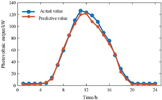
Figure 6 Photovoltaic output prediction.

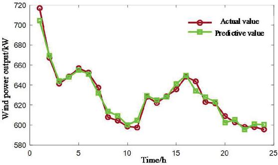
Figure 7 Wind power output prediction.

Table 5 Rules for accuracy classification

Model Accuracy Level:	Level 1	Level 2	Level 3	Level 4
C value range	C $\le$ 0.35	0.35 $<$ C $\le$ 0.5	0.5 $<$ C $\le$ 0.65	C $<$ 0.65

Table 6 Prediction accuracy results in this paper

Prediction Object	Wind Power	Photovoltaic
C	0.1222	0.0811

Analyzing Table 6 reveals that the proposed method attains a first-level accuracy for predicting new energy output. The prediction outcomes align well with the tabulated data, affirming the satisfactory performance of the proposed method. This evaluation not only validates the accuracy of the prediction method used in this study but also demonstrates its capability to provide reliable forecasts for the new energy output within the considered park.

4.3 Analysis of Low-Carbon Economic Scheduling Results

To validate the efficacy of the proposed scheduling method, three distinct scheduling scenarios were formulated and examined, as described below:

(1) Scenario 1: This scenario represents the traditional scheduling mode, where the control does not involve the multi-form energy-intensive-consuming loads, and the utilization of energy storage devices is not considered.

(2) Scenario 2: In this mode, referred to as the source-storage coordination scheduling mode, the control of multi-form energy-intensive-consuming loads is not incorporated, but the utilization of energy storage devices is taken into account.

(3) Scenario 3: This mode, known as the source-load-storage coordination scheduling mode, involves the control of multi-form energy-intensive-consuming loads, coupled with the utilization of energy storage devices.

By evaluating the operating costs associated with each of these scenarios, as presented in Table 7, a comparative analysis can be conducted to assess the economic implications of the proposed scheduling method. These scenarios enable an in-depth exploration of different coordination strategies and their impact on overall system performance, providing valuable insights for practical implementation and decision-making processes.

Table 7 Operating cost of each scenario

	Scenario 3	Scenario 2	Scenario 1
New energy operation and maintenance costs	2412	2468	2872
Operation and maintenance costs of	$-$46	74	0
energy storage equipment
Load regulation cost	$-$239	0	0
Operating cost of gas turbine unit	28006	29011	36158
Total cost of carbon emissions	3639	3767	4685
Total cost	33772	35321	43715

Through a comparative analysis of the park’s operating costs under different scenarios, noteworthy observations can be made. In Scenario 1, which employs traditional dispatch practices, the park encounters significant curtailment of renewable energy, resulting in higher maintenance costs and elevated carbon emissions. Consequently, it exhibits the highest overall operating cost. However, in Scenario 2, by integrating energy storage devices, considering time-of-use electricity prices, and accounting for renewable energy generation, the park witnesses a 19.20% reduction in total cost, a 14.07% decrease in renewable energy maintenance cost, and a 19.60% reduction in carbon emission cost compared to Scenario 1. These outcomes affirm the advantages of source-storage coordination dispatch.

Further building upon Scenario 2, Scenario 3 incorporates the control of controllable multi-form high-capacity loads within the park. In comparison to Scenario 2, Scenario 3 demonstrates a 4.39% reduction in total cost, a 2.27% decrease in renewable energy maintenance cost, and a 3.40% decline in carbon emission cost. This substantiates the benefits of source-load-storage coordinated dispatch and underscores the effectiveness of the proposed method. By considering both the system’s safe operation and the park’s low carbon and economic aspects, the proposed method ensures optimal performance.

Figure 8 visually presents the power output of each micro gas turbine unit under the source-storage-load coordinated dispatch mode. When curtailed wind power is present, the output of each unit is adjusted downwards to accommodate the additional wind power. Conversely, in the absence of curtailed wind power, the output of each unit is increased to compensate for any shortfall in wind power generation.

Figure 9 showcases the control of multi-form high-capacity loads. This study comprehensively accounts for load control characteristics and carbon emissions. Leveraging the combined influence of time-of-use electricity prices and renewable energy generation, the optimization dispatch of multi-form high-capacity loads within the park is realized. When renewable energy generation declines or falls short, the loads are adjusted downwards. Conversely, in the presence of abundant renewable energy generation, the loads are adjusted upwards.

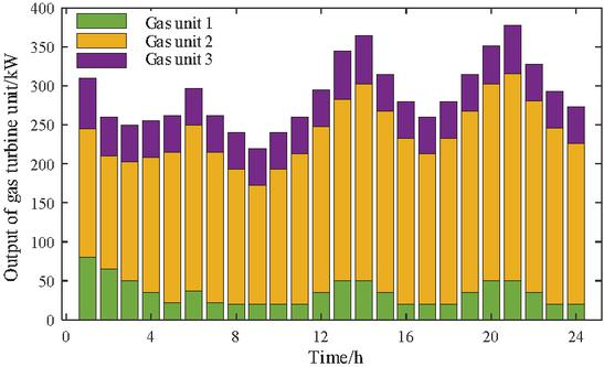
Figure 8 Output of each gas unit.

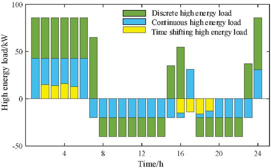
Figure 9 Multi-form energy-intensive load regulation.

Figures 10 to 12 provide valuable insights into the dynamic adjustment of energy storage devices within the park, underscoring their significance in the overall system. Capitalizing on the control of multi-form high-capacity loads and incorporating economic and low-carbon considerations, the park leverages the time-shifting capabilities of energy storage devices to optimize load schedules.

Figure 10 visually presents the operational status of the battery energy storage system. It highlights the crucial role played by the system in storing and releasing energy based on the park’s requirements and external factors. This dynamic operation ensures efficient utilization of available energy resources.

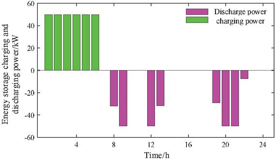
Figure 10 Operation of energy storage system.

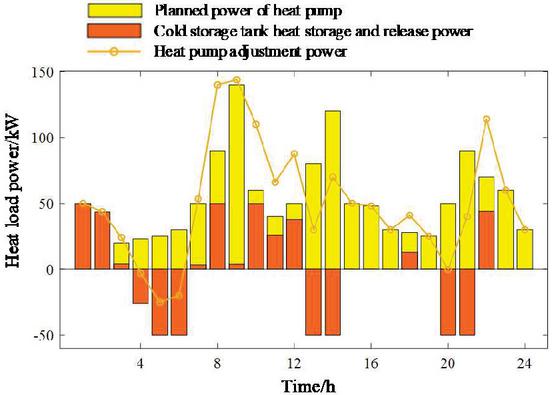
Figure 11 Optimal dispatching results of heat load in the park.

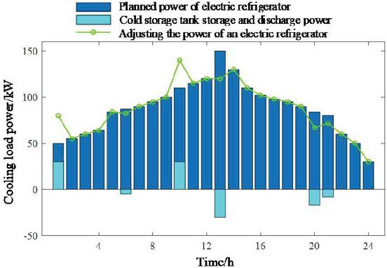
Figure 12 Optimal dispatching results of cold load in the park.

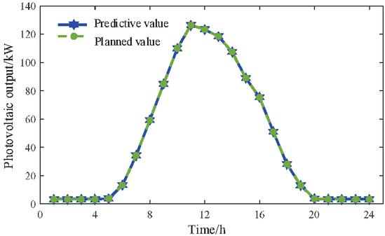
Figure 13 Analysis of PV consumption.

Additionally, Figures 11 and 12 showcase the optimized scheduling outcomes for the park’s heat load and cooling load, respectively. These results reflect the integrated approach that incorporates economic and low-carbon considerations. By exploiting the time-shifting characteristics of energy storage devices, the scheduling algorithm intelligently manages and adjusts the park’s thermal loads to optimize overall performance.

Collectively, Figures 12 to 14 provide a comprehensive visual representation of the adjustment and utilization of energy storage devices within the park, demonstrating their crucial role in enhancing the efficiency, cost-effectiveness, and environmental sustainability of the integrated energy system.

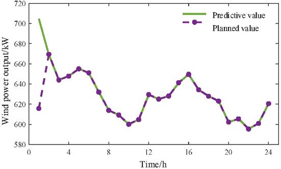
Figure 14 Analysis of PW consumption.

Figure 10 presents the actual charging and discharging behavior of the energy storage system. From 0 to 6 hours, the system is in charging mode, which can be attributed to the substantial wind power output during this interval. The energy storage collaboratively works with demand response to absorb the renewable energy output, thus assimilating electrical energy within this period. Conversely, during the 8 to 13-hour and 19 to 22-hour windows, the system discharges. This discharge corresponds to periods of minimal wind power generation, necessitating the energy storage to work in tandem with demand response to maintain real-time power equilibrium in the electrical system. Hence, electrical energy is released during these intervals. As for Figures 11 and 12, which delineate the scheduling outcomes for heating and cooling loads, the results are computed based on the operational status of the system at each respective time point by the optimization model, lacking a distinct qualitative analysis.

Through the incorporation of the source-load-storage coordination scheduling model outlined previously, this investigation maximizes the utilization of scheduling resources across both the supply and demand aspects. By thoroughly considering the carbon emission characteristics and control capabilities of diverse entities within the park, it successfully attains the objective of low-carbon economic operation, to a certain degree. This comprehensive approach effectively reduces the burden on the park’s gas turbine units for load adjustments, while concurrently augmenting its capacity to integrate renewable energy sources.

The penetration of renewable energy within the park is vividly illustrated in Figures 13 and 14. These figures offer valuable insights into the proportion of renewable energy sources in the overall energy mix. They visually demonstrate the increasing adoption and contribution of renewable energy resources, underscoring the park’s progress towards a more sustainable and environmentally friendly power generation system.

From Figure 13, it is evident that the photovoltaic (PV) day-ahead scheduled output aligns perfectly with the PV day-ahead forecasted output. Over a 24-hour cycle, there is no instance of curtailed solar power. This observation can be attributed to the limited capacity of the photovoltaic generation facility. The peak output in the PV forecasted output curve does not exceed 140 kW, whereas the minimum output of the thermal power units is 127 MW, and the adjustable capacity from the total load itself is around 400 MW. Consequently, through demand response, it is feasible to accommodate the entirety of the PV generation power.

Furthermore, as depicted in Figure 14, during the timeframe from 0 to 3 hours, the wind power output ranges from 670 MW to 704 MW. The wind power alone greatly surpasses the combined maximum values of the total load and energy storage output. Hence, during the 0 to 3-hour period, the demand side cannot absorb all the wind power, necessitating the curtailment of the surplus wind generation. However, from the 3 to 24-hour timeframe, the total wind power output is lesser than that observed during the 0 to 3-hour period. Within this interval, the combined output from wind power and the minimum output from thermal power is less than the sum of the maximum adjustable output from energy storage and the peak of the total load. Therefore, during the 3 to 24-hour period, the demand side can fully accommodate the wind power.

5 Conclusion

This paper delves into a model-predictive, multi-modal high-load zone low-carbon economic scheduling approach. Key conclusions and inferences include:

(1) Innovative Forecasting Model: The study successfully introduced and implemented a GRU renewable energy output forecasting model integrated with ensemble clustering. The essence of this model lies in its ability to extensively harness the characteristic features of renewable energy outputs, achieving top-tier accuracy, thereby standing out from existing forecasting techniques.

(2) Responding to National Energy Strategy Goals: Given the escalating concerns over carbon emissions, the paper factored in the carbon emission characteristics of various entities within the high-load zone and computed their carbon intensity. This represents a proactive response to the nation’s “dual carbon” energy strategy objectives, contributing to the district’s transition towards a low-carbon economy.

(3) Flexible and Comprehensive Dispatching Method: The model-predictive, multi-modal high-load zone low-carbon economic scheduling approach emphasized in this paper accentuates the flexibility of dispatch resources on both supply and demand sides. Furthermore, by holistically considering the carbon emission characteristics and regulatory properties of each district entity, the study achieved the district’s low-carbon economic operation objectives, significantly alleviating the regulatory pressure on gas turbine units and substantially improving the absorption level of renewable energy in the zone.

(4) Explicit Evidential Advantage: Comparative case studies reveal that, in contrast to conventional scheduling models, the method introduced in this paper led to a 23.99% reduction in operational costs for the district and a 23.00% decrease in carbon emission costs, offering empirical support to the efficacy of our approach.

In summary, this study presents a pioneering approach for low-carbon economic operations in districts, demonstrating not only theoretical significance but also immense potential in practical applications.

Acknowledgements

This article is supported by the “Research on Flexible Load Regulation Models and Demand Response Strategies for New Energy Consumption” project, funded by State Grid Liaoning Electric Power Co., Ltd., Anshan Power Supply Company (2022YF-14).

References

[1] China Electric Power Enterprise Federation. 2021–2022 National Power Supply and Demand Situation Analysis and Prediction Report[EB/OL]. [2022-01-27]. http://www.cec.org.cn/menu/index.html?541.

[2] Zheng M, Meinrenken C J, Lackerner K S. Smart house-holds: Dispatch strategies and economic analysis of distributed energy storage for residentital peak shaving[J]. Applied Energy, 2015, 147:246–257.

[3] Li Meicheng, Mei Wenming, Zhang Lingkang, et al. Research on Multi-energy Microgrid Scheduling Optimization Model Based on Renewable Energy Uncertainty[J]. Power System Technology, 2019, 43(04): 1260–1270.

[4] Shang Liqun, Li Hongbo, Hou Yadong, et al. Short-term photovoltaic power generation prediction based on VMD-ISSA-KELM[J/OL]. Power System Protection and Control: 1–11 [2022-06-24].

[5] Yuan Jianhua, Xie Binbin, He Baolin, et al. Short term forecasting method of photovoltaic output based on DTW-VMD-PSO-BP[J/OL]. Acta Energiae Solaris Sinica: 1–8 [2022-06-24].

[6] Wu Chunhua, Dong Along, Li Zhihua, et al. Photovoltaic Power Prediction Based on Graph Similarity Day and PSO-XGBoost[J/OL]. High Voltage Engineering: 1–11 [2022-06-24].

[7] Kang Hongwei, Li Qiang, Yu Shuo, et al. Ultra Short-Term Forecasting for Wind Power Output Based on SA-PSO-BP Algorithm[J]. Inner Mongolia Electric Power, 2020, 38(06):64–68.

[8] Gu Xueping, Zhou Guangqi, Li Shaoyan, Robust Optimization of Load Restoration Scheme Considering Wind Power Prediction Error Correlation[J]. Power System Technology, 2021, 45(10):4092–4104.

[9] Ji Xinge, Li Hui, Ye Lin, et al. Short-term Photovoltaic Power Forecasting Based on Fluctuation Characteristic Mining[J]. Acta Energiae Solaris Sinica, 2022, 43(05):146–155.

[10] Yang Jian, Zhang Li, Wang Mingqiang, et al. Wind power forecasting error simulation considering output level and self-correlation[J]. Electric Power Automation Equipment, 2017, 37(09):96–102.

[11] Shang Qingxiao, Sun Ming. Optimal Dispatching of Power Grid Based on Wind Power and Heat Storage Heating System[J]. Acta Energiae Solaris Sinica, 2021, 42(07):65–70.

[12] Liu Hang, Zhao Haipeng, Wen Ming, et al. Station-grid-load Collaborative Planning Method for Integrated Energy System Considering Flexible Distribution of Load[J/OL]. High Voltage Engineering: 1–13 [2022-06-24].

[13] Zhao Xia, Sun Mingyi, Li Xinyi, et al. Combined load flow of integrated electricity-water system for regional multi-energy service[J]. Electric Power Automation Equipment, 2020, 40(12):23–30.

[14] Gao Xiaosong, Li Gengfeng, Xiao Yao, et al. Day-ahead Economical Dispatch of Electricity-gas-heat Integrated Energy System Based on Distributionally Robust Optimization[J]. Power System Technology, 2020, 44(6):2245–2253.

[15] Qiao Ji, Wang Xinying, Zhang Qing, et al. Optimal Dispatch of Integrated Electricity-Gas System with Soft Actor-Critic Deep Reinforcement Learning[J]. Proceedings of the CSEE, 2021, 41(3):819–833.

[16] Ma Yanfeng, Xie Jiarong, Zhao Shuqiang, et al. Multi-Objective Optimal Dispatching of Active Distribution Network Considering Park-Level Integrated Energy System[J/OL]. Automation of Electric Power Systems, 1–16 [2022-06-23].

[17] Lü Zhilin, Yi Jiaqi, Liu Quan, et al. Low-carbon optimization of integrated energy systems with hydrogen energy utilization and demand response [J/OL] Proceedings of the CSU-EPSA: 1–9 [2023-01-14].

[18] Wang Shiju, Liu Tianqi, He Chuan, et al. Comfort demand response and carbon trading based comprehensive energy economic dispatching in industrial parks[J]. Electrical Measurement & Instrumentation: 1–9 [2022-06-23].

[19] Zhang Bin, Zhang Chijie, Hu Jun, et al. Ensemble Clustering Algorithm Combined With Dimension Reduction Techniques for Power Load Profiles[J]. Proceedings of the CSEE, 2015, 35(15):3741–3749.

[20] Wang Shuai, Du Xinhui, Yao Hongmin, et al. Research on Load Curve Clustering With Multiple User Types[J]. Power System Technology, 2018, 42(10):3401–3412.

[21] Yao Chengwen, Yang Ping, Liu Zejian. Load Forecasting Method Based on CNN-GRU Hybrid Neural Network[J]. Power System Technology, 2020, 44(09):3416–3424.

[22] Xu Xianfeng, Zhao Yi, Liu Zhuangzhuang, et al. Daily Load Characteristic Classification and Feature Set Reconstruction Strategy for Short-term Power Load Forecasting[J]. Power System Technology, 2022, 46(04):1548–1556.

Biographies

Liaoyi Ning, Male, from Anshan City, Liaoning Province, Deputy General Manager of State Grid Liaoning Electric Power Co., Ltd., with a doctoral degree in Power Systems and Automation. His main research areas include optimization and scheduling of power systems, and the secure and stable operation of power systems.

Kai Liang, Male, born in June 1975, from Anshan City, Liaoning Province. Currently employed at State Grid Liaoning Electric Power Co., Ltd., Anshan Power Supply Company. His main research areas are optimization and scheduling of power systems, and active support for the integration of renewable energy.

Bo Zhang, Male, born on January 23, 1994. Currently employed at State Grid Liaoning Electric Power Co., Ltd., Anshan Power Supply Company. Holds a master’s degree in Power Systems and Automation. His main research areas are flexible DC transmission and optimization and scheduling of power systems.

Yang Gao, Male, born on September 21, 1982. Holds a master’s degree in Agricultural Electrification and Automation. Currently employed at State Grid Liaoning Electric Power Co., Ltd., Anshan Power Supply Company. His main research area is optimization and scheduling of power systems.

Zhilin Xu, Male, born on June 20, 1990. Holds a master’s degree in Electrical Engineering. Currently employed at State Grid Liaoning Electric Power Co., Ltd., Anshan Power Supply Company. His main research area is the secure and stable operation of power systems.

Strategic Planning for Energy and the Environment, Vol. 43_2, 251–280.
doi: 10.13052/spee1048-5236.4323
© 2024 River Publishers

Abstract

1 Introduction

2 Renewable Energy Output Prediction Model Based on ICT-GRU

2.1 Obtaining Classification Labels for Renewable Energy Output Characteristics

2.2 Renewable Energy Output Prediction Model Based on ICT-GRU

3 Low-carbon Economic Dispatch Model for Multi-modal High-capacity Energy Park Integrated Energy Systems

3.1 Composition of the Parking Structure

3.2 Low-carbon Economic Dispatch Model

4 Case Study Analysis

4.1 Low-Carbon Economic Dispatch Model

4.2 Analysis of New Energy Output Prediction Accuracy

4.3 Analysis of Low-Carbon Economic Scheduling Results

5 Conclusion

Acknowledgements

References

Biographies