Design of Short-Term Power Load Forecasting Model Based on Deep Neural Network

Qinwei Duan¹, Zhu Chao¹, Cong Fu¹, Yashan Zhong¹, Jiaxin Zhuo^2,* and Ye Liao²

¹Power Dispatch and Control Center, Guangdong Power Grid Co., Ltd, China Southern Power Grid, Guangzhou, 243000, China
²Beijing TsIntergy Technology Co., Ltd, Beijing, 100084, China
E-mail: mikerqw@163.com; chaozhu@gpdc.gd.csg.cn; fucong@gpdc.gd.csg.cn; zhongyashan@gpdc.gd.csg.cn; zhuojx960408@126.com; liaoye1980@126.com
*Corresponding Author

Received 28 June 2023; Accepted 18 October 2023; Publication 09 January 2024

Abstract

In power system operation and planning, the accuracy of short-term power load forecasting is very important. Because of its powerful data processing and modeling ability, deep neural network has become an effective tool to accurately predict short-term power load. In this study, a short-term power load prediction model based on deep neural network is designed, which adopts deep long short-term memory and threshold period unit model, and combines Boosting algorithm for model fusion. The results show that the average absolute percentage error of the model fused by Boosting algorithm is 0.07%, which is 1.02% lower than the average weight method and 0.59% lower than the reciprocal error method. Boosting fusion model can effectively reduce the overall prediction error and maintain high stability of prediction error at peak, plateau and time sampling points, so as to achieve good prediction effect. Specifically, the MAPE of the model fused using Boosting algorithm is 0.07% (95% confidence), which is 1.14% higher than the average weight method and 0.79% higher than the reciprocal error method. The design of short-term power load forecasting model based on deep neural network can provide more accurate prediction for power system operation and planning, and help to improve the operation efficiency and reliability of power system. At the same time, the design and application of this model also provide a new idea and method for the application of deep learning in power system. The introduction of Boosting algorithm further improves the prediction accuracy and stability of the model, which is a major innovation in model design.

Keywords: RNN, global recurrent unit, short term power load, attention LSTM, AdaBoost.

1 Introduction

Short term load forecasting plays a crucial role in broader energy management. Firstly, accurate predictions can help power companies dispatch resources more effectively and reduce operating costs. For example, if the power demand in the next few hours can be accurately predicted, the power company can adjust the power generation in advance to avoid wasting energy or power shortage. Secondly, short-term load forecasting also has an important impact on the stability of the power grid. The stability of the power grid requires a balance between supply and demand. If the prediction is not accurate, it may lead to overload or insufficient power supply, affecting the stable operation of the power grid. Therefore, accurate short-term load forecasting can not only help power companies save costs and improve economic benefits, but also an important means to ensure grid stability and prevent power accidents. Deep neural networks have good performance in predicting nonlinear data such as power loads, but as the number of layers increases, the gradient of deep neural networks is easily lost, making it difficult to handle complex function problems. The most effective method at present is to use DNNs to estimate short-term power load and find the best solution, so as to save maintenance costs while completing daily prediction [1, 2]. In the experiment, we analyzed the prediction curves of DNNs, long short-term memory (LSTMs), global recurrent units (GRUs), and single and combination neural networks (NNs), and compared the relative errors. However, the problem of most DNNs at present is that the number of iterations is tooFor deep neural networks (DNNs), with the increase of the number of layers, the gradient is easy to be lost, which makes it difficult to deal with complex function problems. The most effective method at present is to use DNNs to estimate short-term power load and find the best solution, so as to save maintenance costs while completing daily prediction [1, 2]. In the experiment, we analyzed the prediction curves of DNNs, long short-term memory (LSTMs), global recurrent units (GRUs), and single and combination neural networks (NNs), and compared the relative errors. However, the problem of most DNNs at present is that the number of iterations is too much, and the mean square error and relative error of the evaluation are both greater than the actualFor deep neural networks (DNNs), with the increase of the number of layers, the gradient is easy to be lost, which makes it difficult to deal with complex function problems. The most effective method at present is to use DNNs to estimate short-term power load and find the best solution, so as to save maintenance costs while completing daily prediction [1, 2]. In the experiment, we analyzed the prediction curves of DNNs, long short-term memory (LSTMs), global recurrent units (GRUs), and single and combination neural networks (NNs), and compared the relative errors. However, the problem of most DNNs at present is that the number of iterations is too much, and the mean square error and relative error of the evaluation are both greater than the actual value, which seriously affects the adjustment of the power grid to the energy structure [3]. During the period of rapid change, load fluctuations may increase, which may be caused by a variety of reasons such as emergencies in the system, weather changes or sudden increases in power demand. These load fluctuations may have a negative impact on the stability of the power grid, thus increasing the maintenance and operation costs. The rapid change in power load may be caused by many factors, including system emergencies, weather changes, or sudden increases in power demand. System emergencies may include machine failures, power grid accidents, etc. These events may cause short-term interruptions in power supply, leading to rapid changes in load. Weather changes, such as temperature, humidity, wind power, and rainfall, can also have a significant impact on electricity loads, especially in areas where electricity demand is closely related to weather conditions. Accurately predicting the rapid changes in power load is of great significance for ensuring the stable operation of the power system and reducing operating costs. However, in rapidly changing environments, the difficulty of predicting power loads significantly increases. This requires the study of more efficient prediction methods to cope with rapid changes in power loads. Therefore, different algorithms are required according to different situations. For the short-term load forecasting (STLF) problem, a single NN prediction model can be selected as the initial algorithm choice. Next, the data is divided into different prediction models according to various NNs, and optimized with STLF as the target [4]. The computational examples use real grid data for analysis, and combine AdaBoost model, Attention LSTM model and GRU model to establish the relevant mathematical algorithms and prediction conditions. The proposed optimization model is solved in the grid dataset, ultimately achieving the goals of shortening the construction cycle and reducing costs [5, 6]. It is worth noting that, according to our discussion, the improvement of the accuracy of the proposed model will help power systems make decisions in the real world. This high accuracy can not only provide more accurate short-term and long-term predictions, but also provide more valuable insights for power system operators, thus helping them make more informed decisions. The core of power system operation is the balance of power supply and demand, which requires accurate prediction of power load. Improving the accuracy of short-term power load forecasting models can help power systems make decisions in the real world. High precision forecasting not only provides more accurate short-term and long-term predictions, but also provides more valuable insights for power system operators to make wiser decisions. For example, in the electricity market, power generation companies can develop reasonable generation plans and trading strategies based on load forecasting, to avoid the impact of electricity market price fluctuations caused by power supply and demand imbalance on their economic benefits. In power system scheduling, system operators can develop reasonable power scheduling plans based on load forecasting, improve the operational efficiency of the power system, and reduce operating costs. In addition, for power systems involving renewable energy, due to the significant impact of weather and other factors on the output of renewable energy, there is significant volatility. Therefore, accurate load forecasting is of great significance for formulating reasonable renewable energy scheduling strategies and ensuring stable operation of the power system. Through the above research, the improved accuracy of this model can not only adapt to the rapid changes in power load and provide guarantees for the stable operation of the power system, but also provide practical application value for multiple scenarios such as power market trading, power system scheduling, and renewable energy scheduling. The research will be divided into four parts: firstly, an overview of STLF based on DNN; secondly, STLF research based on deep neural algorithms; then, experimental verification of the second part is carried out; finally, a summary of the research content and its shortcomings is given.

2 Related Works

As NN is a complex nonlinear network structure composed of simulated biological neurons, it integrates nonlinear complex functions into the network structure and approaches arbitrary functions. The Eskandari H team found that the electricity load size is related to external factors such as weather, season, working days, weekends, and holidays. On this basis, a high-precision hourly load forecasting model was established to improve the predictive performance. LSTM and GRU can retain long-term memory. Multi-dimensional feature values were used as inputs and inputted into GRU and LSTM for load prediction per unit time. This method has more advantages than the current research results on STLF both domestically and internationally [7]. Scholars such as Oreshkin B N have focused on deep learning NN to effectively solve the mid-term load forecasting problem in power systems. And it also owns high representing ability for time series with trend, seasonality, as well as significant randomness. This method is easy to implement and train, without the need for data preprocessing, equipping with a prediction error reduction mechanism. The accuracy and prediction bias of this NN are significantly better than other similar networks [8]. Lu, D, and others combined three different machine learning methods to predict the load distribution of the next day’s nodes. On this basis, a data processing method is proposed. This algorithm has better recognition performance than general regression NN. In addition, the predicted load data using this method can also enhance the reliability of the scheme [9]. Chafi Z S et al. put forward a STLF method on the foundation of NN and Particle swarm optimization (PSO) algorithm. This method uses PSO to find the optimal NN parameters to improve the predicting accuracy. Through testing on the Iranian power grid, this method can accurately predict power loads. The method first determines some NN parameters, including the learning rate and hidden layers number. Then, PSO was used to find parameters’ optimal combination. This method can achieve higher predicting accuracy. On this basis, this method was applied to some actual power system data and extensive comparative research was conducted. Compared with other similar methods, this method has advantages in conducting STLF [10]. Jalali S et al. introduced a deep learning based NN for rapid forecasting of power grid loads. This method optimizes the construction and hyperparameters of the network, thereby improving the prediction accuracy of the network. The experiment utilized actual data from the 2018 Australian electricity trading system to verify algorithm effectiveness. This model has obvious advantages compared to other models [11].

In summary, scholars and scientists have made contributions in DNN and STLF. Many improved algorithms have been designed to meet more efficient dataset processing and prediction algorithms. Meanwhile, considering the good data processing performance of the GRU algorithm and the shortcomings of the current STLF, using this method for STLF should have significant application value in resource regulation of the State Grid.

3 Construction of STLF

In the optimization of short-term load forecasting (STLF), deep neural networks (DNN) are successfully applied, and the functions and constraints of actual STLF examples are combined. A deep neural network is a machine learning model capable of representing and learning nonlinear and complex patterns through the connection and interaction of multiple layers of neurons. Using this model, deep and complex patterns in power load data can be captured more effectively, thus improving the accuracy of forecasts. In addition, individual and combined models of deep neural networks (DNN), Long short-term memory (LSTM), and gated cycle units (GRUs) are analyzed in depth. Long Short-term memory (LSTM) and gated cycle unit (GRU) are two special recurrent neural networks (RNNS) that can process sequence data efficiently. Through the combination of deep neural network (DNN), long short-term memory (LSTM) and gated cycle unit (GRU), the time series data of power load can be processed more effectively, and the accuracy of prediction can be further improved. On this basis, the time series formula and other methods are combined to further optimize the prediction model. These methods take advantage of the statistical properties of time series data to provide more information for the training and optimization of predictive models. These research results have an important supporting role for the development and application of power grid load forecasting technology, and also have a positive strategic significance for industrial development.

3.1 Construction of DNN

NN originated in the 1950s, but at that time it was called a perception machine. Although it also has three levels, scholars have found in their research that the fatal drawback of a single level perceptron is that it is difficult to handle complex functions [12]. In the 1980s, with the continuous development of mathematics, the first NN-multi-layer perceptron appeared. This method uses a Continuous function based on sigmoid and tanh to model the response of neurons to external stimuli. To solve this problem, scholars used ReLU, maxout and other Activation function instead of sigmoid, which formed today’s DNN. Except for the Activation function, its structure is no different from the multi-layer perceptron [13, 14]. Expanding RNN along the timeline yields Figure 1.

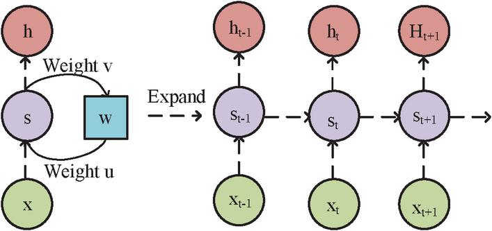
Figure 1 RNN network display.

In Figure 1, RNN is a more reasonable solution when there are long dependencies in the sequence data that cannot be directed. ${x_{1}, \dots, x_{t - 1}$ , $x_{t}, x_{t + 1}, \dots}$ are time series data, $s_{t}$ refers to the sample memory at time $t$ , $w$ stands for the weight between hidden layers, $u$ means the input sample data weight, and $v$ is the output sample weight. From this, Equation (1) can be obtained.

{\begin{matrix} h_{1} = u x_{1} + w s_{0} \\ s_{1} = f (h_{1}) \\ y_{1} = g (v \cdot s_{1}) \end{matrix}

(1)

In formula (1), $f$ and $g$ are activation function. $s_{0}$ and $s_{1}$ are the sample memory at time 0 and 1, respectively. $x_{1}$ is time series data. If advancing at that moment, Equation (2) can be obtained.

{\begin{matrix} h_{t} = u x_{t} + w s_{t} \\ s_{t} = f (h_{t}) \\ y_{t} = g (v \cdot s_{t}) \end{matrix}

(2)

Equation (2) represents the formula for RNN forward propagation, where all parameters are shared. And the length of input and output data may not necessarily be completely consistent. In practical applications, with the prolongation of data timeline, the model depth continues to increase, and RNN cannot learn long-term dependencies well. Usually, Back Propagation Through Time (BPTT) is used to train RNN, which involves the first few steps’ network state [15]. Further advance mapping was performed on sequences ${x_{1}, \dots, x_{t - 1}, x_{t}, x_{t + 1}, \dots}$ through Equation (3).

s_{t} = f (w s_{t - 1} + u x_{t})

(3)

In Equation (3), $s_{t - 1}$ means the previous moment’s mapping state, and $s_{t}$ is the next mapping state. Equation (4) is the loss function gradient with respect to parameter $L_{t}$ EE at time $θ$ .

\nabla_{θ} L_{t} = \frac{\partial L_{t}}{\partial θ} = \sum_{t \leq T} \frac{\partial L_{T}}{\partial s_{T}} \frac{\partial s_{T}}{\partial s_{t}} \frac{\partial s_{t}}{\partial θ}

(4)

In Equation (4), $\nabla_{θ} L_{t}$ stands for the gradient. The matrix $\frac{\partial L_{t}}{\partial θ}$ is divided into $\frac{\partial L_{T}}{\partial s_{T}}$ , $\frac{\partial s_{T}}{\partial s_{t}}$ and $\frac{\partial s_{t}}{\partial θ}$ . Then, the matrix $\frac{\partial s_{T}}{\partial s_{t}}$ is decomposed according to the chain rule in Formula (5).

\frac{\partial s_{T}}{\partial s_{t}} = \frac{\partial s_{T}}{\partial s_{T - 1}} \frac{\partial s_{T - 1}}{\partial s_{T - 2}} \dots \frac{\partial s_{t + 1}}{\partial s_{t}} = f_{T}^{'} f_{T - 1}^{'} \dots f_{t + 1}^{'}

(5)

In Equation (5), when RNN needs to store long-term information, $| f_{t}^{'} | < 1$ is required. But the gradient itself will disappear over time, and the gradient will converge exponentially until 0. When $| f_{t}^{'} | > 1$ , the gradient will explode, and the network will also fall into local instability [16]. For LSTM, after adding three logical control units, Figure 2 shows its structure.

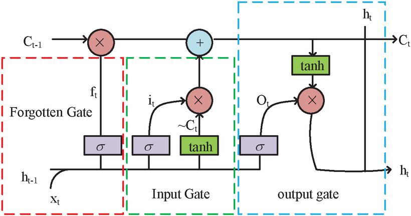
Figure 2 LSTM structure display.

In Figure 2, the gating units of three logical principles are the forgetting gate in red, the input gate in green, and the output gate in blue. The gating device can be seen as a fully connected hierarchy that can be used to update and store LSTM data. The forgetting gate is the most core component in LSTM, used to forget irrelevant information. The input gate performs operations on the input information and stores it in memory. The output gate controls the memory unit to effect the current output value. Equation (6) is the forgetting door activation function.

σ (x) = \frac{1}{1 + e^{- x}}

(6)

In formula (6), $σ (x)$ is a nonlinear activation function, which can describe the information passing degree. When the output value is 0, meaning that information can’t pass through. When this value is 1, meaning that all information can pass through. Equation (7) is the forgetting gate calculation.

f_{t} = σ (W_{x f} x_{t} + W_{h f} h_{t - 1} + b_{f}) = σ (W_{f} V + b_{f})

(7)

In Equation (7), $f$ refers to the forgetting gate, the time step is $f$ , the input of the hidden layer is $x_{t}$ , the output is $h_{t}$ , $W$ means the network weight matrix, and $V$ represents the bias vector. From this workflow to the input gate, Equation (8) is the input gate calculation.

{\begin{matrix} i_{t} = σ (W_{x i} x_{t} + W_{h i} h_{t - 1} + b_{i}) = σ (W_{i} V + b_{i}) \\ {\tilde{c}}_{t} = \tanh (W_{x c} x_{t} + W_{h c} h_{t - 1} + b_{c}) = \tanh (W_{c} V + b_{c}) \\ c_{t} = f_{t} \otimes c_{t - 1} + i_{t} \otimes {\tilde{c}}_{t} \end{matrix}

(8)

In formula (8), $\tanh$ refers to the input gate, $\tanh$ means the input information, $c_{t}$ stands for the memory unit, $\tanh$ is the activation function, and its interval is [ $-$ 1,1]. The gradient around 0 increases with 0 as the center. $\tanh$ converges more quickly, thus following the output value formula of the output gate and hidden gate in Equation (9).

{\begin{matrix} o_{t} = σ (W_{x o} x_{t} + W_{h o} h_{t - 1} + b_{o}) = σ (W_{o} V + b_{o}) \\ h_{t} = o_{t} \otimes \tanh (c_{t - 1}) \end{matrix}

(9)

In Equation (9), $o$ represents the output gate. LSTM’s advantage lies in solving the gradient vanishing and explosion in long time series. To further improve the NN performance, scholars have proposed an attention mechanism. This mechanism simulates the human brain in a specific environment, focusing only on one event while neglecting other things. Its essence is to focus more attention on information that is helpful for solving problems, rather than wasting time in noise. This mechanism can not only record different types of information, but also use information weights to measure the weight of different types of information [17]. Figure 3 shows the working principle of this mechanism.

Figure 3 Display of self attention mechanism.

In Figure 3, the attention mechanism model can assist us in selecting critical inputs for each subsequent stage from the previous hierarchy. The algorithm uses three steps to obtain the main values: firstly, based on the search results of the search results, combined with key information, the similarity score between the two is obtained. Secondly, the initial scores in step 1 were standardized using the maximum soft maximum method to obtain weighting coefficients within the range of [0,1]. Then, the values were weighted and added with different weights to obtain the final result. And from this, the hidden layer state values in Equation (10) were obtained.

{\begin{matrix} α_{k i} = \frac{\exp (S_{k i})}{\sum_{j = 1}^{T_{x}} \exp (S_{k i})} \\ S_{k i} = v \tanh (W h_{k} + U h_{i} + b) \\ C = \sum_{i = 1}^{T_{x}} α_{k i} h_{i} \\ h_{k^{'}} = H (C, h_{k}, x_{k}) \end{matrix}

(10)

In Equation (10), $α_{k i}$ means the attention weight of the hidden layer state of the historical input to the current input. $h_{k^{'}}$ is the hidden layer state value of the final output node. GRU has conducted more in-depth research on the problems faced by LSTM. The design purpose of three “gates” in LSTM is to remove or add input information to the neural unit, thereby controlling the state of the unit [18, 19]. Figure 4 shows the structural units of GRL.

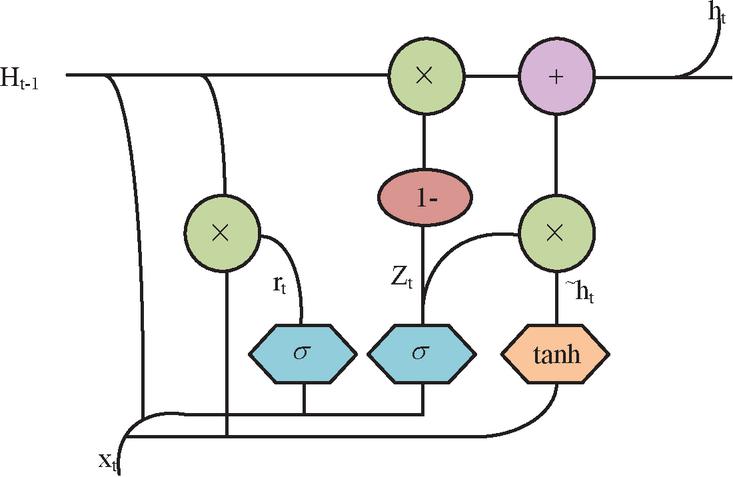
Figure 4 GRU structure display.

In Figure 4, GRU has made improvements to this “gating”. In LSTM, an “update gate” is used instead of an input gate and a forgetting gate, replacing three “gates” with two “gates”. In this way, there are only two “reset gates” left in GRU. Among them, the update gate is responsible for controlling the transmission of past state information in the current state, determining the amount of new state information that includes past state information. The reset gate is responsible for how many states in the past need to be ignored. By resetting the gate, GRU can selectively retain or forget past information. Equation (11) is the internal Formula of GRU.

{\begin{matrix} τ_{t} = σ (W_{τ} h_{t - 1} + U_{τ} x_{t} + b_{τ}) \\ r_{t} = σ (W_{r} h_{t - 1} + U_{r} x_{t} + b_{r}) \\ {\tilde{h}}_{t} = \tanh (W_{τ} (r_{t} h_{t - 1}) + U_{h} x_{t} + b_{h}) \\ h_{t} = (1 - τ_{t}) h_{t - 1} + τ_{t} {\tilde{h}}_{t} \end{matrix}

(11)

In Equation (11), ${\tilde{h}}_{t}$ represents the integration of input and output BB of the previous hidden layer. $W_{τ}$ , $W_{r}$ , $W_{h}$ , $U_{τ}$ , $U_{r}$ , $U_{h}$ , $b_{τ}$ , $b_{r}$ and $b_{h}$ are the units weight matrices. Compared with LSTM, GRU method outperforms LSTM in training effectiveness. Nowadays, GRU technology is widely used in many aspects. For example, GRU networks have replaced LSTM networks and been used for language modeling.

3.2 Construction of STLF for Single NN and Combined NN

For the modeling of a single NN, unlike other models’ 2D data, NN is a 3D data input, and Figure 5 shows the input structure after converting data into 3D data.

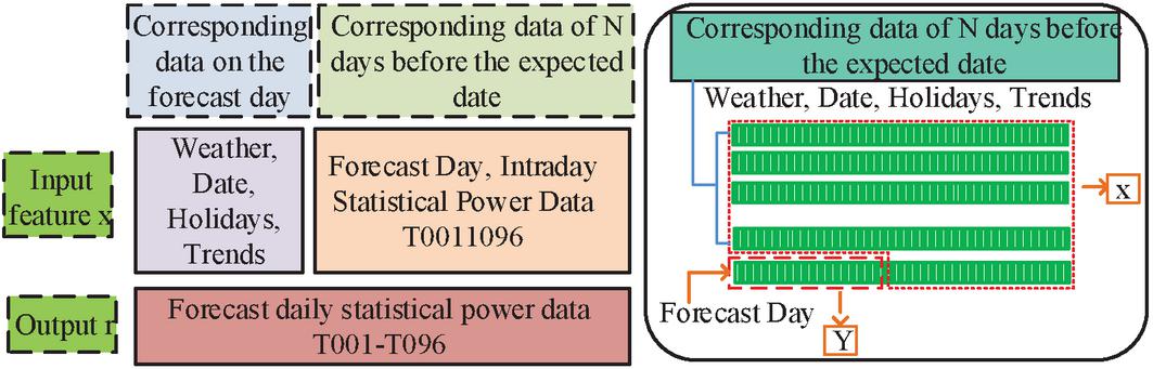
Figure 5 Input structure of neural network model.

In Figure 5, $T$ means the timeline and $F$ is the input feature number. Based on the sampling points of historical load, external factors such as dates, workdays, months, trends, and holidays were predicted for various indicators, and output was made for the sampling points. However, the hidden layer can be single or multiple layers. A single hidden layer network can be used to handle various complex problems. However, compared to this, multiple hidden layers have better promotion ability and higher prediction accuracy. However, as hidden layers increases, it can also cause the network to become more complex and the training time to become longer. So, when selecting hidden layers, it is not only necessary to consider the accuracy of learning, but also the time-consuming calculation. Hide layer nodes based on experience, as shown in Equation (12).

m = \sqrt{l + n} + α

(12)

In Equation (12), $m$ is the hidden layer nodes number, $l$ is the input layer nodes number, $n$ is the output layer nodes number, and $α$ is a constant within 1–10. NN uses activation function, which brings nonlinear factors into the model. Because past power loads were all positive, and the predicted loads were also positive. Therefore, the activation function from NN input layer to hidden layer will use ReLU function. Activation function from hidden layer to output layer will use linear function. Adam optimal method can iteratively adjust NN weights based on training samples, and has the characteristics of simple implementation, fast operation speed, and low storage space requirements. The Ensemble learning prediction model is used to improve, so Figure 6 is the integrated model framework.

Figure 6 Composite frame.

In Figure 6, this method mainly synthesizes the prediction data of two or more individual models to obtain a comprehensive prediction result. By analyzing a single model and analyzing various factors, a single model with good predictive performance was selected and combined [20]. The combination model based on the average weight method is the most simple and convenient. It directly gives the selected single model the same weight without considering any situation in Formula (13).

f_{prei} = \frac{1}{q} (i = 1, 2, \dots, q)

(13)

In Equation (13), $q$ means the model. $i$ is the $i$ -th model weight. And it is further expanded into the integrated model’s formula in Equation (14).

f_{pre} = \sum_{i = 1}^{n} y_{i} f_{prei}

(14)

In Equation (14), $f_{pre}$ means the predicting result of ensemble method, and $f_{prei}$ is the prediction result of the $i$ -th model. This method utilizes polynomial joint modeling to reduce joint modeling errors and improve prediction accuracy by weighting individual patterns with small deviations. The error used in the combined model is the average absolute percentage error, also known as MAPE. Equation (15) is the integrated model of the reciprocal error method.

{\begin{matrix} ω_{1} = \frac{ε_{2}}{ε_{1} + ε_{2}} \\ ω_{2} = \frac{ε_{1}}{ε_{1} + ε_{2}} \\ f_{pre} = ω_{1} f_{pre 1} + ω_{2} f_{pre 2} \end{matrix}

(15)

In Equation (15), $ω_{i}$ is the weight coefficient, and $ε_{i}$ is each model error. The integration method refers to a meta algorithm that combines multiple machine learning techniques into a prediction model. Currently, this method includes a type of parallelization algorithm represented by Bagging, where individual learners do not have strong dependencies with other learners and can be generated simultaneously. Boosting, on the other hand, is a typical sequential algorithm where each learner has strong dependencies and needs to be generated sequentially. The study aims to use XGBOOSt as the foundation and BOOSTling’s integrated learning method to fuse individual prediction models. Compared with other machine learning methods, XGBoost has two major advantages. Firstly, while improving the predicting accuracy, the complexity and subsequent pruning have been optimized, making it less prone to overfitting and more robust. Secondly, the computational efficiency of this mode has been significantly improved. In theory, this new modeling method has accuracy, robustness, and efficiency.

4 Analysis of STLF Results

When the scale of deep learning networks changes, their computational load and memory overhead also increase. At present, the prediction model based on Root-mean-square deviation (RMSE) and Average Relative Error (MAPE) is reasonable. However, the quality of the results is not high and not strict enough to guarantee the optimal solution. Therefore, it is difficult to achieve ideal results when solving complex optimization problems. When a single forecasting model is affected by external factors, it will produce lag, leading to poor forecasting performance. In contrast, the prediction results obtained by the integrated algorithm have higher computational efficiency and larger space. So it is more suitable for combinatorial optimization problems.

4.1 Analysis of Prediction Models Based on a Single NN

The experimental environment was chosen as Python version 3.7 and programmed in Spyder. We used Keras and TensorFlow tools to construct a deep learning model. The dataset is sourced from the State Grid of Xi’an City, Shaanxi Province, China, and is based on the actual load data of the power grid. The size of the dataset is 16 GB/M, and its features include background information, data type, data source, etc. To evaluate the performance of the model, a series of experiments were conducted, covering 675 sampling points over a 7-day period. When evaluating model performance, two key indicators were used: root mean square error (RMSE) and mean absolute percentage error (MAPE). The root mean square error (RMSE) is used to reflect the difference between the predicted and actual values of the model, and its magnitude can effectively measure the stability of the model. The average absolute percentage error (MAPE) is mainly used to evaluate the accuracy of a model, which reflects the percentage error between the predicted value and the actual value of the model, and its magnitude is directly related to the accuracy of the model. The parameter table is shown in Table 1.

Table 1 Parameter information of the experiment

Parameter	Description	Detailed Description
Programming Environment	Python 3.7	Python 3.7 is used for programming due to its strong stability and compatibility.
Programming Tool	Spyder	Spyder is chosen as the programming tool, as it is a powerful environment for Python scientific computing.
Deep Learning Framework	Keras, TensorFlow	Keras and TensorFlow are chosen as the deep learning frameworks for their powerful functionalities and ease of use.
Dataset Source	National Power Grid of Xi’an City, Shaanxi Province, China	The dataset is based on actual load data from the national power grid in Xi’an City, Shaanxi Province, China.
Dataset Size	16GB/M	The dataset size is 16GB/M, which is relatively large and beneficial for model training.
Dataset Features	Background information, data types, data sources, etc.	The dataset features include background information, data types, data sources, etc., providing a wealth of training features.
Experiment Scope	675 sampling points within 7 days	The experiment is carried out within 7 days, covering 675 sampling points, which helps to comprehensively evaluate the model’s performance.
Evaluation Metrics	Root Mean Square Error (RMSE), Mean Absolute Percentage Error (MAPE)	RMSE and MAPE are chosen as evaluation metrics as they can comprehensively reflect the stability and accuracy of the model.
Role of RMSE	Reflects the difference between the model’s predictions and actual values, measures model stability	RMSE is used to quantify the error between the model’s predictions and actual values, the smaller the value, the better the model’s stability.
Role of MAPE	Reflects the percentage error between the model’s predictions and actual values, evaluates model accuracy	MAPE is used to evaluate the average relative error of the model’s predictions, the smaller the value, the higher the model’s accuracy.

In Table 1, in order to comprehensively evaluate the performance of the model, in addition to RMSE and MAPE, other evaluation indicators such as MAE and MPE can also be considered. In addition, the training time and prediction time of the model can also be evaluated to understand its efficiency. Figure 7 shows each NN single model’s structure.

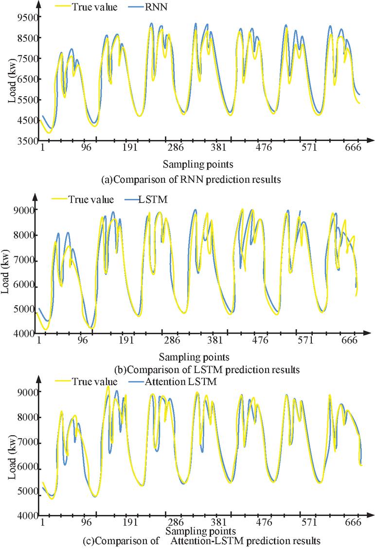
Figure 7 Comparison of RNN, LSTM, and Attention LSTM model predictions.

Figure 7 shows the one week prediction results of recurrent NNSTLF. From Figure 7(a), the load trend predicted by RNN is generally similar to the real curve. In the sampling point area where the electricity consumption changes steadily, the prediction is more accurate. However, in the peak and valley values where the load fluctuates greatly, the prediction error significantly increases. In Figure 7(b), from load curve’s overall prediction results, compared with the RNN model, LSTM has improved overall prediction accuracy and maximum prediction performance. From Figure 7(c), this single model also improves the fitting degree of the load peak, and its error fluctuation is relatively stable, with overall good prediction performance. In LSTM, the use of attention mechanisms can effectively improve the performance of general LSTM models, thereby demonstrating the advantages of attention mechanisms. Figure 8 shows the range of P-values for each point per week.

Figure 8 Comparison of p-values for pursuit point MAPE.

Figure 8 shows the p-value comparison of the pursuit point MAPE. Compared with the attention LSTM model, the prediction error of the GRU model is statistically more stable (p $<$ 0.05). However, in the later prediction stage, the p-value of the MAPE of the GRU model significantly increased at 8 am during the peak electricity consumption (p $<$ 0.05), indicating a significant decrease in its predictive performance during this time period. On the contrary, the predictive advantage of the attention LSTM model in the early peak time zone is statistically more significant (p $<$ 0.05). And the predictive advantage of the attention LSTM model in the early peak time zone will be more pronounced in Figure 9.

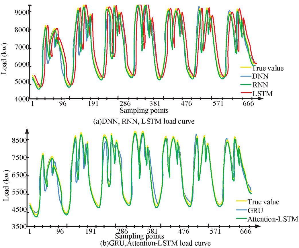
Figure 9 Comparison of single neural network model results.

From Figure 9, it can be observed that each independently constructed neural network model exhibits results that are consistent with the actual load variation trend. Among these models, the predictive values of deep neural network models exhibit significant fluctuations, especially when the sampling points vary greatly, and their predictive performance is not ideal. In contrast, RNN exhibits good predictive performance in situations where load fluctuations are relatively stable, but in the stage where the prediction time is relatively long, there is a significant deviation between its predicted results and the actual load, and the prediction curve shows a “Z” shaped trend. For models with long-term memory characteristics, such as the Attention LSTM mechanism, LSTM, and GRU, they have higher prediction accuracy for stable samples and exhibit better fitting ability for invariant samples. After comparing with the other three models, it can be concluded that the prediction results of LSTM and GRU models are closer to the actual situation. Electricity prediction, as a method of improving prediction accuracy using non-stationary sequence data, faces the challenge of not being able to achieve completely error free prediction. Therefore, the focus of researchers has shifted towards reducing power operating costs and improving power supply quality to address this challenge.

4.2 Analysis of Prediction Model Based on Combination NN

When designing a short-term power load prediction model based on deep neural networks, the core step of model evaluation is to use a preprocessed historical dataset during the model training stage, which includes records of power load and other related influencing factors. The output of the model is a prediction of future power loads. Secondly, the evaluation of model performance is mainly based on selected performance indicators, which typically include mean absolute error (MAE), mean square error (MSE), root mean square error (RMSE), and mean absolute percentage error (MAPE). These indicators can quantify the accuracy of model predictions, and the smaller the error, the higher the prediction accuracy. Specifically, MAE measures the average absolute deviation between predicted values and actual values; MSE and RMSE are more sensitive to large errors by targeting the average and square root of the square of the prediction error; MAPE represents the ratio of prediction error to actual value, and is commonly used to compare prediction results of different dimensions or units. Finally, during the model testing phase, the prediction performance of the model for future unknown data is simulated by verifying the dataset. These datasets were not used for model training. By comparing the predicted results with the actual results, the model’s generalization ability to invisible data can be evaluated. This evaluation process effectively verifies the predictive performance of the model and provides a basis for improving the model. AdaBoost, Attention LS TM, and GRU were combined. The combination methods are average weight method, error reciprocal method and combination method based on Ensemble learning. The experiment selected 675 sampling points from a total of one week of real power grid data in 2020 for validation, and selected MAPE and RMSE as evaluation indicators. Different single prediction models and different combination methods based on the AdaBoost-GRU model were presented, and the results included corresponding confidence or reliability descriptions. Among them, the prediction results of the long-term memory neural network model have a higher confidence level compared to other single machine learning models. Specifically, the MAPE of the model fused using the Boosting algorithm is 0.07% (95% confidence), which is 1.14% higher than the average weight method and 0.79% higher than the reciprocal error method. This data shows that our combined model has not only significantly improved prediction accuracy, but also has an advantage in reliability.

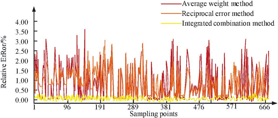
Figure 10 Comparison of Relative Errors for Predicting Weekly Points Based on Different Combination Methods of AdaBoost-GRU.

Figure 10 shows the relative errors of 672 sampling points during prediction period using different combination algorithms based on AdaBoost-GRU. Overall, three combination modes have improved prediction results, and the average weighting method has improved overall prediction performance. However, there are still significant errors in the peak and flat valley sampling points. The error inversion method can improve overall prediction effect, but it cannot completely solve the problem of poor prediction performance when the load changes sharply. Boosting fusion model can effectively reduce overall prediction errors, and maintain high stability of prediction errors at peak, flat valley, and over time sampling points, thus achieving good prediction results. Taking into account the non-linear relationship in the combined model based on MAPE results is more conducive to the correction and improvement of the model results.

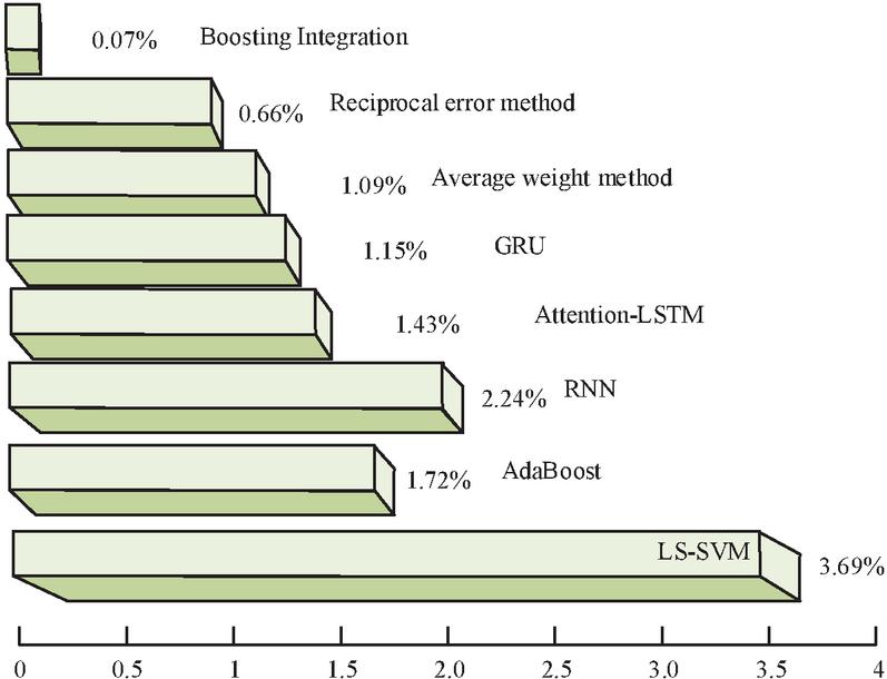
Figure 11 Comparison of MAPE for various models.

In Figure 11, MAPE results of different single prediction models and different combination methods based on AdaBoost-GRU are presented. Among them, NN with long-term memory is superior to other single machine learning models. The model MAPE fused with Boosting algorithm is 0.07%, which is a decrease of 1.02% compared to the average weight method and 0.59% compared to the reciprocal error method. The prediction accuracy has been significantly improved, and this combined model has an advantage. Figure 12 shows the comparative prediction results of a single model.

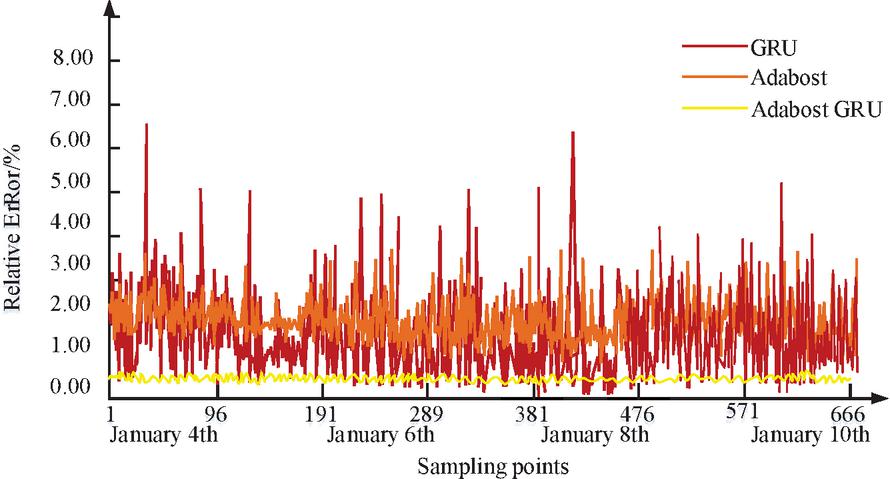
Figure 12 Comparison of relative errors of AdaBoost, GRU, and AdaBoost-GRU prediction points on a weekly basis.

In Figure 12, based on the XGBoost fusion model proposed by Boosting, the weights of different individual models are dynamically adjusted to achieve a combination of prediction results for the two models. From the prediction result graph, we can see that after fusion, better learning of the structural features of different models has been carried out, resulting in a more stable prediction error output. Compared with the single model without Boosting method, this method has significantly improved the prediction accuracy of load peak and valley turning periods. By using the Boosting algorithm and combining the advantages of AdaBoost and GRU methods, more accurate forecasting of the power grid can be achieved, thus saving a lot of operating costs.

5 Conclusion

In short-term load forecasting (STLF), we adopt a forecasting model based on single algorithm and integrated algorithm, and verify various indicators. The results of the comparison experiment show that compared with Attention LSTM, the relative prediction error of GRU is more stable when comparing MAPE of tracking points. However, in the subsequent forecast phase, the MAPE of the GRU will increase at 8 o’clock during the morning peak of electricity consumption. The predicted value of DNN generally has great fluctuation, especially when the sampling point changes significantly, the predicted value is not ideal. Compared with the other three models, the LSTM and GRU models’ predictions are closer to the actual situation. The three combined models all improve the prediction results, and the average weighting method improves the overall prediction results. However, there are still significant errors in the sampling points of useful peaks and flat valleys. Error inversion method can improve the overall prediction effect. However, it can not completely solve the problem of poor predictive performance when the load changes sharply. NN for long-term memory outperforms other single machine learning models. The MAPE of the model integrated with Boosting algorithm is 0.07%, which is 1.02% lower than the average weight method and 0.59% lower than the reciprocal error method. Prediction accuracy has been significantly improved, and combined models have advantages. Future studies can explore the influence of timeliness factors on STLF. Therefore, the results of this study have great reference value for guiding STLF. It has been ensured that the conclusions effectively summarize the key findings of the study. The drawback of this study is that in practical applications, timeliness is also a key consideration in addition to the need for efficient budgeting of short-term power loads. In the actual operation of power system, the change of power load is often fast and complicated, which requires the power load prediction to be not only accurate, but also fast. However, when considering the accuracy of the prediction model, the timeliness of prediction is not fully taken into account in this study. The importance of this contribution cannot be overlooked, especially in relation to the optimization and timeliness of predictive models. In the power system, the accuracy and timeliness of load forecasting is very important, because it directly affects the operating efficiency and stability of the power system. Any method and technology that can improve the accuracy and timeliness of load forecasting has important practical value. However, although a short-term power load forecasting model based on deep neural networks is proposed in this study and its superiority is verified by experiments, there are still many areas that need further research. For example, how to further optimize the structure and parameters of the prediction model to improve the accuracy of the prediction; How to adjust the operation strategy of prediction model according to the demand of practical application to improve the timeliness of prediction; And how to effectively integrate the prediction model with the components and functions of other power systems to improve the practicability of prediction. It is hoped that future researchers can further explore these aspects to further improve the accuracy and practicality of the prediction.

Fundings

The research is supported by the Science and Technology Project of China Southern Power Grid Corporation: Research and Application Development of Load Forecasting Technology in Regions with New Energy Permeability Exceeding 40% – Topic 3: Research on Intelligent Bus Load Forecasting Technology Considering Source Load Interaction and Application Development of Regional Load Intelligent Forecasting System, (No. 036000KK52210065(GDKJXM20210096).

References

[1] N. Zafar, I. U. Haq, J. R. Chughtai. Applying hybrid LSTM-GRU model based on heterogeneous data sources for traffic speed prediction in urban areas. Sensors, 22(9): 3348–3390, 2022.

[2] P. L. Seabe, C. R. B. Moutsinga, E. Pindza. Forecasting cryptocurrency prices using LSTM, GRU, and bi-directional LSTM: A deep learning approach. Fractal and Fractional, 7(2): 203–210, 2023.

[3] A. Mellit, A. M Pavan, V. Lughi. Deep learning neural networks for short-term photovoltaic power forecasting. Renewable Energy, 172(Jul.): 276–288, 2021.

[4] S. Li, W. Luan, C. Wang, Y. Chen, Z. Zhuang. Degradation prediction of proton exchange membrane fuel cell based on Bi-LSTM-GRU and ESN fusion prognostic framework. International Journal of Hydrogen Energy, 47(78): 33466–33478, 2022.

[5] M. E. Karim, M. Foysal, S. Das. Stock Price Prediction Using Bi-LSTM and GRU-Based Hybrid Deep Learning Approach Proceedings of Third Doctoral Symposium on Computational Intelligence: DoSCI 2022. Singapore: Springer Nature Singapore, 16(Jun.): 701–711, 2022.

[6] T. Ahmad, D. Zhang. A data-driven deep sequence-to-sequence long-short memory method along with a gated recurrent neural network for wind power forecasting. Energy, 239(Jan.15 Pt.B): 122109.1–122109.20, 2022.

[7] H. Eskandari, M. Imani, M. P. Moghaddam. Convolutional and Recurrent Neural network Based Model for Short-Term Load Forecasting. Electric Power Systems Research, 195(4): 107173.1–107173.14, 2021.

[8] B. N. Oreshkin, G. Dudek, P. Peka, E. Turkina. N-BEATS neural network for mid-term electricity load forecasting. Applied Energy, 293(1): 116918.1–116918.13, 2021.

[9] D. Lu, D. Zhao, Z. Li. Short-term nodal load forecasting based on machine learning techniques. International Transactions on Electrical Energy Systems, 31(9): e13016.1–e13016.24, 2021.

[10] Z. S. Chafi, H. Afrakhte. Short-Term Load Forecasting Using Neural Network and Particle Swarm Optimization (PSO) Algorithm. Mathematical Problems in Engineering, 2021(Pt.17): 5598267.1–5598267.10, 2021.

[11] S. Jalali, S. Ahmadian, A. Khosravi, M. Shafie-Khah, J. P. S. Catalao. A Novel Evolutionary-based Deep Convolutional Neural Network Model for Intelligent Load Forecasting. IEEE Transactions on Industrial Informatics, 17(12): 8243–8253, 2021.

[12] X. Serrano-Guerrero, M. Briceo-León, J. M. Clairand, G. Escrivá-Escrivá. A new interval prediction methodology for short-term electric load forecasting based on pattern recognition. Applied Energy, 297(Sep.1): 117173.1–117173.13, 2021.

[13] W. Yang, J. Shi, S. Li, Z. Song, Z. Zhang, Z. Chen. A combined deep learning load forecasting model of single household resident user considering multi-time scale electricity consumption behavior. Applied Energy, 307(Feb.1): 118197.1–118197.18, 2022.

[14] Y. Lu, G. Wang, S. Huang. A short-term load forecasting model based on mixup and transfer learning. Electric Power Systems Research, 207(Jun.): 107837.1–107837.9, 2022.

[15] M. N. Fekri, H. Patel, K. Grolinger, V. Sharma. Deep learning for load forecasting with smart meter data: Online Adaptive Recurrent Neural Network. Applied Energy, 282(Jan.15 Pt.A): 116177.1–116177.17, 2021.

[16] X. Wu, C. Dou, D. Yue. Electricity load forecast considering search engine indices. Electric Power Systems Research, 199(11): 107398.1–107398.9, 2021.

[17] L. Sun, T. Liu, Y. Xie, D. Zhang, X. Xia. Real-time power prediction approach for turbine using deep learning techniques. Energy, 233(Oct.15): 121130.1–121130.18, 2021.

[18] M. Lehna, F. Scheller, H. Herwartz. Forecasting day-ahead electricity prices: A comparison of time series and neural network models taking external regressors into account. Energy Economics, 106(Feb.): 105742.1–105742.15, 2022.

[19] Y. Cao, X. Zhou, K. Yan. Deep Learning Neural Network Model for Tunnel Ground Surface Settlement Prediction Based on Sensor Data. Mathematical Problems in Engineering, 2021(Pt.37): 9488892.1–9488892.14, 2021.

[20] Y. Guo, Z. Mustafaoglu, D. Koundal. Spam Detection Using Bidirectional Transformers and Machine Learning Classifier Algorithms. Journal of Computational and Cognitive Engineering, 2(1): 5–9, 2023.

Biographies

Qinwei Duan obtained his BE in Electrical Engineering & Automation from Sichuan University in 2013. He obtained his MEng in Electrical Engineering from the University of Nottingham in 2014 and Ph.D from the University of Hong Kong in 2018. Presently, he is working in Guangdong Power Grid Power Dispatch and Control Center, China Southern Power Grid. His areas of interest are power system dispatch, load forecast, power balance, and renewable energy integration.

Zhu Chao obtained his BE and Master degree in Electrical Engineering & Automation from South China University of Technology in 2008 and 2011, respectively. Presently, he is working in Guangdong Power Grid Power Dispatch and Control Center, China Southern Power Grid. His areas of interest are power system dispatch, load forecast, power balance, and electricity market.

Cong Fu obtained his BE in Electrical Engineering & Automation from HUST in 2010. He obtained his Master degree in Electrical Engineering from Wuhan University. Presently, he is working in Guangdong Power Grid Power Dispatch and Control Center, China Southern Power Grid. His areas of interest are long term power balance, and renewable energy integration.

Yashan Zhong obtained her BE in Business Administration from North China Electric Power University in 2014. She obtained her Master degree in Technology Economy and Management from North China Electric Power University in 2017. Presently, she is working in Guangdong Power Grid Power Dispatch and Control Center, China Southern Power Grid. Her areas of interest are power system dispatch, load forecast, power balance, and system economic operation.

Jiaxin Zhuo obtained his BE in Electrical Engineering & Automation from Southwest University in 2018. He obtained his Master degree in Agricultural electrification and automation from Southwest University in 2021. Presently, he is working in Beijing TsIntergy Technology Co., Ltd. His areas of interest are power system dispatch and load forecast.

Ye Liao obtained his BE in Applied Chemistry from Nanchang University in 2003. He obtained his Master degree in Software Engineering from Beihang University in 2015. Presently, he is working in Beijing TsIntergy Technology Co., Ltd. His areas of interest are power system dispatch, load forecast, and power balance.

Strategic Planning for Energy and the Environment, Vol. 43_2, 425–452.
doi: 10.13052/spee1048-5236.43211
© 2024 River Publishers