Soil Moisture Prediction Model Based on Improved GRU Recurrent Neural Network
Guowei Wang*, Chunying Wei, Li Yan and Jian Li
College of Information Technology, Jilin Agricultural University, Changchun 130118, China
E-mail: guowei0wang@sina.com
*Corresponding Author
Received 30 August 2023; Accepted 01 November 2023; Publication 09 January 2024
Abstract
Soil moisture plays a crucial role in land water and energy cycles, and has a certain impact on weather and climate change. In agricultural production, crop moisture status can be determined based on soil moisture, and timely and effective irrigation strategies can be formulated to ensure grain yield while saving water resources, maximizing the value of agricultural water resource utilization, and achieving sustainable development. Therefore, the accuracy of soil moisture prediction has important research value for many fields such as agriculture and climate. In this paper, the super parameters of GRU Recurrent neural network are optimized by intelligent seagull optimization algorithm using a small number of influencing factors, namely, atmospheric temperature, atmospheric humidity, rainfall and soil moisture data, and a soil moisture prediction model is established. The model was used to predict soil moisture for the next 12 hours, 24 hours, 36 hours, and 48 hours, respectively. The final experiment showed that the model in this paper had better predictive effect on soil moisture, with the best predictive evaluation index data being MAPE (12h) 4.4120%, R2 (12h) 0.94605, and RMSE (12h) 1.9998; By comparing the prediction results of multiple time steps vertically, it was found that the prediction accuracy of the model in this paper decreased more smoothly, meeting the requirements of soil moisture prediction.
Keywords: GRU recurrent neural network, seagull optimization algorithm, soil moisture prediction.
1 Introduction
The soil is the loose surface layer on the earth’s land and at the bottom of shallow water, which can produce Viridiana. It plays an important role in land resources, is an important base for crop growth, is the data of agricultural production, and plays a very important role in the ecosystem. As a physical quantity that distinguishes the degree of soil dryness and wetness, soil moisture, also known as soil moisture content, is a fundamental parameter in the formation, transformation, and consumption of surface water resources. It plays a crucial role in regional ecosystems, plant growth, and other processes. Currently, there are three main ways to obtain soil moisture information: on-site observation [2], remote sensing inversion, and model simulation. The field observation method mainly collects soil moisture information at a certain time and location through a soil moisture monitor. The soil moisture information obtained by this method has high accuracy and strong timeliness, but the data obtained by this method usually only represents the soil moisture situation near the observation point, and the spatial representativeness of the data is poor [3], which cannot obtain the soil moisture situation in a large area. The use of remote sensing inversion method to obtain soil moisture is cost-effective, has a larger detection range, and has a longer monitoring cycle and higher temporal resolution. However, there are inevitably certain shortcomings, such as difficulty in obtaining meteorological data and poor inversion results in areas with high vegetation coverage density. There are many types of prediction models in the model simulation method, and in recent years, with the continuous development of machine learning, more and more researchers have applied this method to the study of soil moisture prediction. The research results also indicate that this method can find soil moisture rules within the research scope and achieve its prediction purpose.
At present, the prediction models for soil moisture mainly include empirical models, time series, neural networks, combination models, etc. Thiemann et al. selected a Bayesian recursive estimation method for predicting soil moisture content, which describes the prediction based on the probability of different output values of the model. During the prediction process, the uncertainty of parameter estimation values is continuously updated. This model has been applied to the Mississippi River Basin with good results [4]. Yan et al. used the multiple Law of Return method to analyze the correlation between the average temperature, relative humidity, precipitation and other meteorological factors and soil moisture, and built a soil moisture prediction model, and verified that the model simulation value and the measured value have good consistency [5]. Yang et al. proposed using BP neural network to predict soil moisture based on data with time series characteristics, and achieved ideal prediction results [6]. Bai Dongmei et al. used time series data as the research object and constructed a soil moisture prediction model using autoregressive method. After verification, the model can effectively predict soil moisture content [7]. Mukhlisin et al. compared and analyzed the predictive effects of regularized and non-regularized neural network models on the saturated water content of weathered granite soil layers, and the results showed that the regularized neural network model had better predictive performance [8]. Zai et al. selected precipitation, evaporation, relative humidity, and groundwater depth as input factors for the neural network model to construct a soil moisture prediction model. The prediction accuracy of the model was verified to be high [9]. Yu et al. proposed a hybrid CNN GRU model for predicting soil moisture at the roots of corn, providing a decision-making basis for irrigation [10]. Xue et al. constructed soil moisture prediction model using combinatorial algorithms improves the accuracy of soil moisture prediction [11]. Ge et al. combined the BP neural network algorithm, Random Forest algorithm and Extreme learning machine algorithm in the machine learning method with spectral data to establish a soil moisture inversion prediction model. The results show that the three models can better inverse and predict the soil moisture in the study area, and the Extreme learning machine algorithm model has the best effect [12].
In summary, researchers both domestically and internationally have conducted extensive research on soil moisture prediction and achieved certain research results. However, due to the comprehensive influence of multiple factors on soil moisture, current research on soil moisture prediction models has their own advantages and disadvantages, although they are all as close to the actual soil moisture values as possible, However, there are still some prediction models that require a large capacity of elements to be measured, or have high requirements for parameter acquisition and model establishment. Therefore, further research and exploration are needed to establish more accurate and universal soil moisture prediction models.
This study utilizes time series data such as continuously collected air temperature and humidity, rainfall, and soil moisture to develop a soil moisture prediction model. Due to the powerful nonlinear mapping ability of neural networks, they can quickly find the relationships between variables from massive data under the premise of uncertain relationships between variables. Compared to general neural networks, GRU recurrent neural networks are very effective in processing data with sequence features, while also solving the problems of partial gradient disappearance and gradient explosion. And Shewalkar et al. analyzed and compared three types of recurrent neural networks, RNN, LSTM, and GRU, and tested them using datasets with long-term dependency characteristics. The experimental results showed that GRU and LSTM recurrent neural networks were relatively similar in performance and accuracy, and the error rate was significantly lower compared to RNN recurrent neural networks. At the same dataset, GRU recurrent neural networks converged faster [13]. Therefore, in this study, the GRU recurrent neural network was used as the basic model for soil moisture prediction.
2 Establishment of a Soil Moisture Prediction Model
2.1 GRU Recurrent Neural Network
Gate Recurrent Unit (GRU) neural network is a simplified structure based on LSTM Recurrent neural network unit proposed by Ge et al. in 2014 [14], that is, on the basis of LSTM Recurrent neural network, the gate structure is optimized, the forgetting gate and the input gate are combined into “update gate”, and the output results can be taken as the memory state, and are continuously transmitted backwards, without giving additional memory state, The training speed of the network has been improved while ensuring accuracy [15]. Compared with the three gates of LSTM Recurrent neural network, GRU Recurrent neural network only has update gate and reset gate, as shown below:
(1) Change the input gate, forgetting gate, and output gate into update gate and reset gate.
(2) Set the unit state C of LSTM Recurrent neural network_ Merge t and output into one state h_ t. Figure 1 shows the unit structure of GRU Recurrent neural network neurons.
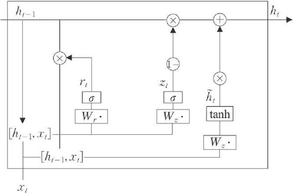
Figure 1 GRU neuron structure.
The workflow of GRU Recurrent neural network can be summarized as follows:
(1) Reset door Connect reset door to the previous hidden layer state . The size of its weight affects the amount of information that needs to be forgotten in the previous hidden layer state. The calculation formula is as follows:
| (1) |
In the formula: is matrix multiplication, is the weight matrix of the gate structure, and is bias; represents the connection of a matrix, is the sigmoid Activation function.
(2) Candidate status at the current moment After calculating the reset gate, obtain the candidate state of the hidden layer at the current time . The calculation formula is as follows:
| (2) |
Among them, represents the multiplication of the corresponding elements of the matrix. If the value of is large, it indicates that there is also more information saved by the hidden layer in the previous moment, then, the greater the impact will have.
(3) Update Gate is the update gate in the network, which controls the transmission of the previous hidden state to the current hidden state in the network. The amount of information in indicates that the greater the weight, the more information needs to be saved. The calculation formula is as follows:
| (3) |
(4) The output layer is in the current state Finally, output the hidden layer state at the current time. It represents the amount of information that should be extracted from the previous information state and the amount of information that needs to be retained from the candidate state . By and jointly controls the output. The calculation formula is as follows:
| (4) |
2.2 Seagull Optimization Algorithm
Dhiman et al. were inspired by the migration and attack behavior of seagull populations and proposed the Seagull Optimization Algorithm (SOA) in 2019 [16]. This algorithm mainly simulates the behavior of seagulls during migration and attack, such as avoiding collisions, finding the best position, and attacking to find the optimal solution. Compared with other optimization algorithms, seagull optimization algorithm has less parameters to adjust and better global search ability, so it has the advantages of fast Rate of convergence and high optimization accuracy [17]. The process of its algorithm is as follows:
2.2.1 Migration behavior
At the current stage, the algorithm simulates the position transformation of seagulls during their migration behavior, that is, the process of moving from the current position to the next position. This process belongs to the global search stage, and any seagull should meet the following conditions:
(1) Avoiding collisions In order to avoid collisions with other individual seagulls in the seagull population, variable A is introduced to calculate the current position of the seagull after transformation, that is, the individual position update of the seagull.
| (5) |
Among them, represents a new location that will not collide with other search seagulls, represents the current position of the seagull, x represents the current number of iterations, and A represents the movement behavior of the seagull in a specific search space.
| (6) |
Among them, the introduction of controls the frequency of variable A, which varies from linearly decreases to 0. The value of is 2.
(2) Best position direction After avoiding positional conflicts with other seagulls, seagulls will fly towards the location of seagulls with the best fitness value.
| (7) |
Among them, represents the position where each seagull moves towards the best fitness seagull . The value of B is random and is responsible for achieving an appropriate balance between global and local searches. The calculation method for B is:
| (8) |
Among them, is a random number between [0,1].
(3) Approaching the optimal position After the seagull reaches a position where it does not collide with other seagulls, it flies in the direction of the best position, thereby reaching a new position to complete the position update.
| (9) |
2.2.2 Attack behavior
During the attack phase, seagulls launch attacks on food during flight, which is manifested by using their wings and weight to control their flight height. During the hunting process, seagulls continuously adjust their attack angle and speed, thereby exhibiting a spiral motion pattern in the air. This process belongs to the local search phase.
| (10) | |
| (11) | |
| (12) | |
| (13) |
Among them, , , and are plane coordinates, r is the radius of each spiral motion of the seagull, and k represents the angle value of the seagull’s spiral motion, which is a random number within the range of . u and v are constants describing their helical states, and e is the base of Natural logarithm.
In summary, the attack location of seagulls can be calculated, namely:
| (14) |
2.2.3 Algorithm steps
The main calculation steps of the Seagull Optimization Algorithm are as follows:
(1) Initialization parameters: Set the number of seagull populations and the initial position of seagulls. Set parameters , , and . Among them, , , ;
(2) Calculate the fitness value of each seagull;
(3) Calculate the new location for seagulls to complete their migration behavior using formulas (5)–(9);
(4) Calculate the final position of seagulls using formulas (10)–(14);
(5) Update the optimal seagull position and fitness values;
(6) When , if the termination condition is met, proceed to the next step; otherwise, skip to step (3);
(7) Output the global optimal seagull position and fitness value.
2.3 GRU Recurrent Neural Network Based on Seagull Optimization Algorithm
Although GRU Recurrent neural network has a simple structure and few parameters, it is still the same as other neural networks, and the super parameters involved still need to be set manually. In order to avoid the influence of experience and randomness on manual setting of super parameters, this study uses seagull optimization algorithm to optimize the three super parameters of GRU Recurrent neural network, namely, the number of hidden layer nodes, the initial Learning rate and L2 regularization coefficient, to improve the prediction accuracy.
In this study, the steps of optimizing GRU Recurrent neural network (SOA-GRU model for short) based on seagull optimization algorithm SOA are as follows:
(1) Initialize the parameters of the seagull optimization algorithm, including the number of populations, number of iterations, number of hyperparameters to be optimized, and the upper and lower limits of hyperparameters to be optimized;
(2) Build GRU Recurrent neural network and set its parameters, including the number of input and output layer nodes, the number of hidden layers, etc;
(3) The super parameters of the GRU Recurrent neural network to be optimized are transferred to the seagull optimization algorithm as the object to be optimized.
(4) Calculate the fitness value of seagulls and complete position updates.
(5) Determine whether the seagull optimization algorithm has reached the maximum number of iterations. If the conditions are met, the obtained optimal parameter value will be used as the global optimal solution. Otherwise, it will return to step (4) until the conditions are met.
(6) The optimal results obtained by seagull optimization algorithm are used as the super parameters of GRU Recurrent neural network, namely, the number of hidden layer nodes, initial Learning rate and L2 regularization coefficient. Then the optimized GRU Recurrent neural network is trained and soil moisture is predicted.
3 Results and Analysis
3.1 Data Collection
The data in this study is collected by physical sensor equipment in Qijia Town, Shuangyang District, Changchun City, Jilin Province. The variables include soil moisture, rainfall, atmospheric temperature, and atmospheric humidity. The data is recorded every four hours from June 2018 to June 2020. However, due to equipment failure, some data have problems and become invalid data. In addition, seasonal factors will have a certain impact on the prediction results, So the final valid data selected for the study were from June, July, and August 2018 and 2019. Table 1 below shows some experimental data.
Table 1 Partial collection data
| Atmospheric | Atmospheric | Soil | ||
| Serial Number | Temperature (C) | Humidity (%RH) | Rainfall (ml) | Moisture (%RH) |
| 1 | 18.1 | 100.0 | 1.6 | 34.1 |
| 2 | 19.2 | 94.8 | 2.0 | 34.6 |
| 3 | 25.9 | 64.7 | 2.4 | 34.9 |
| 4 | 19.9 | 88.2 | 3.2 | 34.8 |
| 5 | 17.6 | 100.0 | 3.4 | 34.9 |
| 6 | 15.5 | 100.0 | 3.4 | 35.0 |
| 7 | 13.1 | 100.0 | 0.0 | 35.0 |
| … | … | … | … | … |
3.2 Model Parameter Settings
After conducting experimental exploration using variables from different consecutive periods before a certain time, it was determined that the input variables of the model were atmospheric temperature, atmospheric humidity, rainfall, and soil moisture data from 18 consecutive periods before a certain time. Since the data recording time interval for each period was 4 hours, there were a total of 72 input variables. And normalize all variable data to improve the predictive performance of the model. At the same time, the order of the input sample dataset is disrupted to prevent overfitting and improve the generalization ability of the model. The sample ratio between the training and testing sets is set to 8:2.
In the GRU algorithm, the Adam algorithm is selected to adaptively adjust the learning rate of different parameters, ensuring that the gradient can swing and descend within the normal range, keeping the parameters relatively stable and improving the descent rate. The selected activation function is the ReLU function. The learning rate adjustment method used in this study is the piecewise constant attenuation method, and the learning rate is set to decay by 0.2 times after every 850 iterations. The maximum training frequency of the GRU recurrent neural network is 2000, and the model can achieve better fitting results.
In the SOA algorithm, the population number of seagulls is set to 10, and the number of iterations is 30. The value domains of the three super parameters to be optimized, namely, the number of hidden layer nodes, the initial Learning rate, and the L2 regularization coefficient are [10100], [0.0001,0.002], and [1e-10,1e-2].
3.3 Experimental Environment
The operating environment of the experimental platform for this study is shown in Table 2.
Table 2 Experimental environment parameter table
| Environmental | Parameter Values |
| Hardware | (1) CPU: Intel(R) Core (TM) i7-10875H CPU @2.30GHz |
| (2) GPU: NVIDIA GeForce RTX 2060 | |
| Software | (1) Operating system: Windows 10 64 bit |
| (2) Development tool: Matlab 2020a |
3.4 Experimental Results
After processing the original data, the data of atmospheric temperature, atmospheric humidity, rainfall, and soil moisture in the first 72 hours are used as input variables, and the data are normalized to make the value range between [0,1]. The SOA-GRU models are used to predict and explore the soil moisture data in different time periods in the future, and the time steps are set as 12 h, 24 h, 36 h and 48 h respectively.
After testing, when the number of hidden layer nodes is 64, the learning rate is 0.001, and the L2 regularization coefficient is 1e-5, the model achieves better prediction performance. The prediction results are as follows:
The comparison between the predicted and true values of soil moisture in the test set with a predicted time step of 12 hours is shown in Figure 2. The red curve represents the true value, and the blue curve represents the predicted value.
It can be seen from Figure 2 that both models can capture the change trend of soil moisture, and the fitting ability of the same model will decline when the prediction time step gradually increases; Under the same prediction time step, the SOA-GRU model has a relatively better fitting effect on soil moisture.
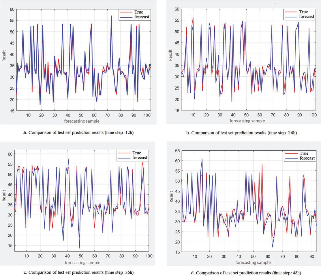
Figure 2 Comparison of test set prediction results.
3.5 Result Analysis
Comparing the model studied in this article with the Bayesian improved GRU model (BOA-GRU), various evaluation indicators are obtained as shown in Table 3.
Table 3 Model evaluation index value
| MAPE | RMSE | R | ||||||||||
| Model | 12h | 24h | 36h | 48h | 12h | 24h | 36h | 48h | 12h | 24h | 36h | 48h |
| SOA-GRU | 4.41 | 5.25 | 6.65 | 7.02 | 1.99 | 2.36 | 3.15 | 3.83 | 0.95 | 0.945 | 0.91 | 0.85 |
| BOA-GRU | 5.66 | 5.33 | 6.66 | 7.04 | 2.78 | 3.47 | 3.99 | 4.44 | 0.93 | 0.89 | 0.86 | 0.82 |
The analysis results of the evaluation indicator data in Table 3 are as follows:
(1) RMSE is used to measure the predictive accuracy of the model. The smaller the value of RMSE, the higher the prediction accuracy of the model; On the contrary, it indicates that the prediction accuracy of the model is relatively low. Compared with the BOA-GRU model, the RMSE of the SOA-GRU model decreased by 28.24%, 32.12%, 21.06%, and 13.79% when the prediction time steps were 12 h, 24 h, 36 h, and 48 h, respectively. The RMSE of both models shows a gradually increasing trend with the extension of time steps.
(2) MAPE is used to measure the advantages and disadvantages of a model. The closer its value is to 0, the higher the quality of the model; The closer the value is to 100%, the poorer the quality of the model. Comparing the MAPE of the same prediction time step of the SOA-GRU model and the BOA-GRU model, when the time step is 12 hours, the MAPE of the SOA-GRU model is reduced by 22.11% compared to the BOA-GRU model. The MAPE of the two models is not significantly different in the other three-time steps. In addition, as the prediction time step increases, the MAPE of the two models also shows a gradually increasing trend, like RMSE.
(3) R is used to measure the degree of fit of the model. When the time steps are at the same time, the R of the SOA-GRU model is greater than that of the BOA-GRU model. When the predicted time steps are 12 h, 24 h, 36 h, and 48 h, the R of the SOA-GRU model is increased by 1.66%, 5.85%, 6.51%, and 3.33% compared to the BOA-GRU model, respectively. The R values of the SOA-GRU model were all above 0.94 within 24 hours of prediction, and their R values were all above 0.90 within 36 hours of prediction; Compared to the R of the BOA-GRU model, only when the time step is 12 hours, its R value is greater than 0.90, which is 0.93059. In addition, comparing the decrease in fitting degree of the two models with the extension of prediction time, it can be found that the R decrease of the SOA-GRU model is smaller, ranging from 0.94605–0.84508, a decrease of 10.67%; The R of the BOA-GRU model decreased by 12.12%, with a range of 0.93059–0.81783.
The established model was used to predict soil moisture for 10 times at 24 and 48 hours, and the predicted results are shown in Table 4.
Table 4 Soil nutrient prediction results
| 24 h | 48 h | |||||
| Serial Number | Predicted | True | Error | Predicted | True | Error |
| 1 | 24.1 | 23.6 | -0.5 | 52.2 | 52.8 | 0.6 |
| 2 | 34.7 | 30.9 | -3.8 | 38.8 | 50.9 | 12.1 |
| 3 | 22.8 | 22.8 | 0 | 35.5 | 35.9 | 0.4 |
| 4 | 36.2 | 35.3 | -0.9 | 32.4 | 35 | 2.6 |
| 5 | 50.1 | 51.2 | 1.1 | 34 | 33.9 | -0.1 |
| 6 | 26.1 | 23.5 | -2.6 | 25.7 | 23.3 | -2.4 |
| 7 | 24.32 | 24.2 | -0.12 | 33 | 33.1 | 0.1 |
| 8 | 30.2 | 24.2 | -6 | 32.1 | 31.8 | -0.3 |
| 9 | 33.15 | 32.9 | -0.25 | 36.5 | 34.2 | -2.3 |
| 10 | 34 | 32.1 | -1.9 | 27.3 | 30.1 | 2.8 |
According to Table 4, the average relative error for 24 hours is 1.6778, and the average relative error for 48 hours is 2.37. Compared with the results in the references, the results shown in Table 5 are obtained.
Table 5 Comparison of average errors
| Evaluating | SOA-GRU | Reference | Reference | Reference | Reference [12] | ||
| Indicator | 24 h | 48 h | [6] | [8] | [10] | 24 h | 48 h |
| Average relative | 1.678 | 2.37 | 2.45 | 4.25 | 4.27 | 3.22 | 4.06 |
| error | |||||||
From Table 5, it can be seen that the soil moisture prediction model established in this article has smaller average relative error and higher prediction accuracy compared to the reference literature.
4 Discussion
Predicting soil moisture in advance is an important basis for soil moisture management and decision-making, therefore, early and accurate prediction of soil moisture is very important. This article establishes a soil moisture prediction model by optimizing the GRU recurrent neural network. The results show that the soil moisture prediction model proposed in this study based on the optimized GRU recurrent neural network can grasp the trend of soil moisture changes and has good prediction results. In terms of model improvement, researchers mainly focus on optimizing the hyperparameters of GRU networks, such as using particle swarm optimization [18], LSTM optimization [19], CNN optimization [20], and AlexNet optimization [21]. These optimization models have achieved good results in different fields, therefore, using optimization algorithms to improve GRU networks is feasible. The Seagull algorithm has the advantages of simple algorithm structure and strong applicability, making it convenient for algorithm improvement and fusion. The simple algorithm structure of the Seagull algorithm brings lower algorithm complexity and efficient computing power [22], which has enabled the algorithm in this paper to achieve faster prediction capabilities. In terms of soil moisture prediction, this model also has higher accuracy and lower error compared to the models in the reference literature. Therefore, the model established in this article can meet the time and accuracy requirements for soil moisture prediction.
However, in this study, only the effects of air temperature, humidity, and rainfall on soil moisture were considered. In fact, there are many factors that affect soil moisture, such as evaporation. In future research, more practical factors need to be considered in order to further improve the prediction accuracy of the model.
5 Conclusion
This study is based on the significant impact of soil moisture on climate, meteorology, agriculture, and other aspects, as well as its significance in various research fields. It uses partial meteorological data and soil moisture data to predict future soil moisture. The seagull optimization algorithm is used to optimize the super parameters of GRU Recurrent neural network, namely, the number of hidden layer nodes, the initial Learning rate and L2 regularization coefficient, and establish the SOA-GRU soil moisture prediction model. Use the established SOA-GRU soil moisture prediction model to predict soil moisture for the next 12 hours, 24 hours, 36 hours, and 48 hours, respectively. By analyzing the prediction results and model evaluation indicators, it was found that the SOA-GRU model has better prediction performance. When the prediction time step is 12, R2 is 0.94605; The RMSE and MAPE (100%) were 1.9998 and 4.4120, respectively, achieving the goal of using a small number of influencing factors to predict soil moisture.
Acknowledgment
Fund Project: This research was funded by Industrialization research project of Jilin Provincial Department of Education (Grant No. JJKH20220341CY).
Statements & Declarations
Competing Interests: The authors have no relevant financial or non-financial interests to disclose.
Data Availability: The datasets generated during and/or analysed during the current study are available from the corresponding author on reasonable request.
References
[1] Nie Yan, Ma Zeyue, Zhou Xiaofeng, Yu Lei, Yu Jing. Research on Soil Moisture Inversion and Monitoring in the Aksu River Basin. Journal of Ecology, 2019, 39(14):5138–5148.
[2] Zhai Hui. Study on the influence mechanism of water and organic matter on the transformation of soil selenium forms. Northwest A&F University, 2021.
[3] Hao Zhen. Research on soil moisture inversion technology based on multi-source data collaboration. Lanzhou Jiaotong University, 2017.
[4] Thiemann M, Trosset M, Gupta H, et al. Bayesian recursive parameter estimation for hydrologicmodels. Water Resources Research, 2001, 37(10):2521–2535.
[5] Aguilera H, Moreno L, Wesseling J G, et al. Soil moisture prediction to support management in semiarid wetlands during drying episodes. CATENA, 2016,147:709–724.
[6] Yan Changrong, Shen Huijuan, He Wenqing, Liu Shuang, Liu Qin. Research on soil moisture prediction model based on multiple regression method. Journal of Hubei University for Nationalities (Natural Science Edition), 2008(3):241–245.
[7] Haoxiong Yang, Chuan Zhao, Xinjian Du, Jing Wang. Risk Prediction of City Distribution Engineering Based on BP. Systems Engineering Procedia, 2012, 5.
[8] Bai Dongmei, Guo Mancai, Guo Zhongsheng, Chen Yanan. Application of Time Series Autoregressive Model in Soil Moisture Prediction. Soil and Water Conservation in China, 2014(2):42–4569.
[9] Muhammad Mukhlisin, Ahmed El-Shafie, Mohd Raihan Taha. Regularized versus non-regularized neural network model for prediction of saturated soil-water content on weathered granite soil formation. Neural Computing and Applications, 2012,21(3):543–553.
[10] Zai Songmei, Guo Dongdong, Han Qibiao, Wen Ji. Prediction of soil moisture based on artificial neural Network theory theory. China Agricultural Bulletin, 2011,27(8):280–283.
[11] Yu Jingxin, Zhang Xin, Xu Linlin, Dong Jing, Zhangzhong Lili. A hybrid CNN-GRU model for predicting soil moisture in maize root zone. Agricultural Water Management, 2021,245:106649.
[12] Xue Ming, Wei Bo, Li Juan, Chen Cihao, Huang Minhui, Zou Linxin. Research on soil moisture prediction method based on improved BP neural network and support vector machine. Soil Bulletin, 2021,52(4): 793–800.
[13] Apeksha Shewalkar, Deepika Nyavanandi, Simone A. Ludwig. Performance Evaluation of Deep Neural Networks Applied to Speech Recognition: RNN, LSTM and GRU. Journal of Artificial Intelligence and Soft Computing Research, 2019,9(4):235–245.
[14] Ge Xiangyu, Ding Jianli, Wang Jingzhe, Wang Fei, Cai Lianghong, Sun Huilan. Estimation of soil moisture content based on competitive adaptation weighted sampling algorithm coupled with machine learning. Journal of Optics, 2018,38(10):393–400.
[15] Kyunghyun Cho, Bart van Merrienboer, Çaglar Gülçehre, Fethi Bougares, Holger Schwenk, Yos hua Bengio. Learning Phrase Representations using RNN Encoder-Decoder for Statistical Machine Translation. CoRR, 2014, abs/1406.1078.
[16] Zhao Jianpeng, Zhang Aijun, Cai Chengfei, Su Yinhong. Research on Prediction of Wave Dip Angle Based on Gated Recurrent Networks. Foreign Electronic Measurement Technology, 2019,38(5):96–100.
[17] Gaurav Dhiman, Vijay Kumar. Seagull optimization algorithm: Theory and its applications for large-scale industrial engineering problems. Knowledge-Based Systems, 2018,165:169–196.
[18] Jiang Siwei, Sun Yan, Chen Jing, et al. Improved Particle Swarm Optimization GRU Network for Grain Storage Temperature Prediction. Computer and Digital Engineering, 2023,51(05):1036–1041+1156.
[19] Qiao Xiaodan, Zheng Wengang, Zhang Xin, et al. Research on the Prediction Method of Sunlight Greenhouse Environment Based on LSTM-GRU. Jiangsu Agricultural Science, 2022,50(16):211–218.
[20] Chen Yihao, Li Mingwei, An Xiaogang, et al. Research on the Intelligent Prediction Method of Dam Deformation Based on Chaotic Quantum Bat CNN-GRU. Journal of Harbin Engineering University: 1–12 [2023-09-25].
[21] Zhu Hainan, Li Fengshuo, Sun Huazhong et al. Short term load forecasting method for distribution networks based on improved AlexNet GRU deep learning network. Power Capacitors and Reactive Power Compensation, 2023,44(04):48–5461.
[22] Li Yuanhang. Comparative Study on the Optimization Performance of Seagull Optimization Algorithm and Whale Optimization Algorithm. Modern Information Technology, 2021,5(03):67–71
Biographies

Guowei Wang, PhD, associate professor, works at Jilin Agricultural University. Executive Director of Jilin Provincial Operations Research Association and Executive Director of Jilin Provincial Smart Agriculture Association. The main research areas include artificial intelligence and computer agriculture applications, intelligent decision-making systems, and GIS. Led 3 projects of the Provincial Department of Science and Technology, 1 project of the Provincial Agricultural Commission, participated in 9 national level projects, and 8 provincial-level scientific research projects; Received 1 first prize and 2 second prizes for scientific and technological progress in Jilin Province. Obtained 4 national invention patents, 6 utility model patents, and 24 software copyright registrations; Write over 30 scientific research papers.

Chunying Wei, Master of computer science and technology. Her research interests include deep learning and agricultural big data analysis.

Li Yan, lecturer, teacher at the Mathematics Department of the School of Information Technology, Jilin Agricultural University. Main research directions: Information theory, data mining. Guiding students to participate in mathematical modeling competitions has won one national second prize and multiple provincial awards in Jilin. Guide students to participate in two innovation and entrepreneurship program projects. Participated in 3 projects of the Jilin Provincial Department of Science and Technology, 5 other department level projects, and 1 Jilin Provincial Innovation Team. Hosted or participated in 4 school level educational reform projects. Published 9 papers, obtained 2 utility model patents, and applied for 14 software copyright registrations.

Jian Li, a member of the Communist Party of China, holds a Ph.D. in Engineering, a professor, and a doctoral supervisor. He is currently the Vice Dean of the School of Information Technology at Jilin Agricultural University, the leader of the first level discipline authorized for a Master’s degree in Computer Science and Technology, and the leader of the Data Science and Big Data Technology major. Expert in the evaluation of the National Natural Science Foundation project, communication evaluation expert of the Degree Center of the Ministry of Education, member of the Jilin Province Higher Education Undergraduate Teaching Guidance Committee, and Jilin Province Science and Technology Commissioner.
Strategic Planning for Energy and the Environment, Vol. 43_2, 381–400.
doi: 10.13052/spee1048-5236.4329
© 2024 River Publishers