Intelligent Energy System and Power Metering Optimization Based on the Energy Plan Model
Ce Peng1, FanQin Zeng2, Youpeng Huang2, Zhaopeng Huang3,* and Xinming Mao4
1Guangdong Power Grid Corporation, Guangzhou, 510180, Guangdong, China
2Metrology Center of Guangdong Power Grid Corporation, Guangzhou, 510062, Guangdong, China
3Foshan Power Supply Bureau of Guangdong Power Grid Corporation, Foshan, 528000, Guangdong, China
4China Energy Engineering Group Guangzhou Electric Power Design Institute Co., Ltd, Guangzhou, 510663, Guangdong, China
E-mail: superdavid@21cn.com
*Corresponding Author
Received 24 December 2023; Accepted 20 January 2024
Abstract
With the national carbon neutrality and carbon peaking policies proposed one after another, this paper proposes intelligent Energy system design and power metering based on the Energy Plan model. In this paper, the Energy PLAN model is proposed as the basic model for energy development planning during the 14th Five-Year Plan period, and the simulation calculation is carried out for the energy system in 2020. The research shows that there is a large gap between the peak and valley of power load, the peak time of power supply and demand does not match, and the response-ability of the energy supply department is poor. Thus, the problems to be solved in the development of energy are determined. In addition, the accuracy of the model is further verified by comparing the actual data with the simulation results of Energy PLAN, and the direction of energy structure reform is determined. By coupling the NSGA-II (Non-dominated Sorting Genetic Algorithms-II) algorithm with the development model, a dual-objective multi-time scale scheduling model is established, which aims at the minimum operating cost and the best energy and environmental benefit coefficient. Secondly, the proposed model is solved using the NSGA-II algorithm. In order to ensure the diversity of solutions and promote the Pareto front approach to the ideal Pareto front, the fuzzy dominance method is used to perform a fast non-dominated sorting of the population, and the maximum satisfaction method is used to select the Pareto optimal compromise solution. Example analysis shows that when the power demand level is L*-L*-L*, the power input under “H-M”, “M-L” and “H-L” scenarios is 106.02 10, 102.73 10 and 94.2 10 GWh, respectively. However, when the power demand level is H*-L*-L*, the power input is always 142.64 10 GWh. With the decrease in the transmission rate, the measurement data obtained by the user’s electric acquisition platform becomes less and less, and the performance of state estimation becomes worse. When , the proposed model still maintains a high estimation accuracy.
Keywords: Energy plan, energy structure, energy and environmental benefits, NSGA-II, electric power measurement.
1 Introduction
The acceleration of urbanization and industrialization leads to the consumption of resources and energy, while the imbalance between energy demand and energy consumption, low energy efficiency, and unreasonable energy structure also aggravate the damage of the greenhouse effect on environmental benefits [1]. Therefore, it is necessary to expand the utilization of clean energy, improve the development rate of clean energy, and adopt and research and develop emerging technologies in the exploitation and use of fossil energy and fuel to make it cleaner and more efficient [2]. The growth in energy demand will be met through a variety of supplies including oil, gas, coal and renewables. As the transition to a low-carbon energy system continues, the energy mix is changing, with renewables and gas gaining in importance relative to oil and coal. To optimize the energy supply side, it is urgent to meet the energy demand and carry out the low-carbon and energy-saving energy transformation.
At present, to solve the problem of high battery life loss during wind power tracking and scheduling planning, Yu Yang et al. proposed a battery energy storage group control strategy to reduce the life loss and used the designed revolving door algorithm based on the improved Tenniushu search algorithm to obtain the optimal compression offset, and then extracted the wind power trend [3]. Lu Quan et al. established a coupling balance analysis model of a provincial electric-thermal integrated energy system with multiple flexible resources. In this model, similar equipment is aggregated first to simplify the complexity of the problem, and system security and stability constraints such as system backup and minimum operation mode are considered through a daily heuristic unit combination [4]. Li Chenxi et al. established an energy system development planning model based on the superstructure modeling method, which can be used for the development path planning aiming at carbon peak. The model takes the regional energy system structure and main infrastructure as the planning starting point, and comprehensively considers the possibility and mutual substitution of various energy supply, transformation, transmission, storage, and consumption technologies at different periods during the planning period, to obtain the low-carbon development technology path with the optimal total cost of the energy system [5]. To realize the multi-energy complementary advantages and cascade utilization of the integrated energy system of the park containing cold, heat, electricity, and gas, Xu Yan et al., based on the project example of an integrated energy system of a park, conducted a detailed case analysis from the aspects of resource assessment, load forecasting, integrated energy system modeling, optimization algorithm solving, regional energy supply station, and pipe network planning principles [6]. Cheng Jifeng et al. quantified the transaction risk by applying the conditional value-at-risk theory and proposed an automatic adjustment method of the risk coefficient to achieve risk control, to obtain the optimal surplus power inter-provincial trading plan [7].
In this paper, the Energy PLAN model is proposed as the basic model for energy development planning during the 14th Five-Year Plan period, and the simulation calculation is carried out for the energy system in 2020. The research shows that there is a large gap between the peak and valley of power load, the peak time of power supply and demand does not match, and the response-ability of the energy supply department is poor. Thus, the problems to be solved in the development of energy are determined. In addition, the accuracy of the model is further verified by comparing the actual data with the simulation results of Energy PLAN, and the direction of energy structure reform is determined. By coupling the NSGA-II algorithm with the development model, a dual-objective multi-time scale scheduling model is established, which aims at the minimum operating cost and the best energy and environmental benefit coefficient. Secondly, the NSGA-II algorithm is used to solve the proposed model. To ensure the diversity of solutions and promote the approximation of the Pareto frontier to the ideal Pareto frontier, the fuzzy dominance method is applied to fast non-domination ranking of populations, and the maximum satisfaction method is applied to select the optimal compromise solution of Pareto.
2 Construction of Energy Development Model
2.1 Energy PLAN Model Analysis
The Energy PLAN model, an advanced modeling tool developed specifically for the analysis of renewable energy systems, is promoted at Aalborg University, Denmark.It is an hourly deterministic input-output model designed for regional and national energy system analysis on a yearly basis. It is often used for technical and economic analysis of energy system construction investment in different countries, and helps scholars to provide corresponding policy suggestions for national or regional energy strategic planning [8]. The model focuses on different energy system simulation strategies and emphasizes synergies between the various sectors of the entire energy system. It requires a large amount of data and high accuracy when modeling all sectors of the entire energy system.
The Energy PLAN model combines the input of different sectors with the output results of the model – sub-energy consumption, critical additional electricity production, and carbon dioxide emissions. It is divided into two parts: energy production and energy consumption. The model structure is shown in Figure 1. The model can perform technical or economic simulations for different sectors, including electricity, personal and central heating, cooling systems, industry, transportation, energy storage systems, and more [9]. At the same time, Energy PLAN emphasizes the impact of different energy strategies or policies on the energy, environment, and economy of a country or region. On this basis, the regional energy system is forecasted and evaluated, and the optimal operation strategy is determined. It is suitable for the design of future power system structures.
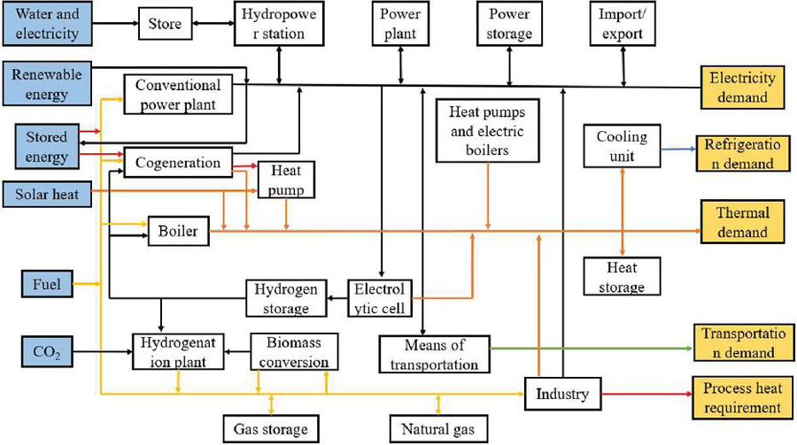
Figure 1 Energy PLAN structure block diagram.
Different from the traditional Energy system simulation model, the Energy PLAN model pays more attention to renewable energy. It can accurately simulate a variety of renewable power generation, including hydropower, wind power, photovoltaic, biomass, and more. At the same time, based on the historical power generation data of the system, the volatility and hourly distribution of renewable energy are considered. Therefore, it is possible to conduct a complete simulation of the Sichuan power system which is dominated by clean energy [10]. In addition, the Energy PLAN integrates various emerging technologies such as pumped storage power stations, hydrogen storage, and high-temperature heat pumps in the optimization of renewable energy systems, and adopts electric energy alternative technologies (such as electric vehicles, smart vehicles, and grid interconnection, etc.) in the optimization of the transportation sector. Therefore, when simulating the integration of high levels of renewable energy resources, the Energy PLAN model can be used because it takes into account the overall and technical details of each technology required in the study.
Technical operation refers to the system simulation by adopting different technical simulation strategies, which are usually used to design and analyze large-scale complex energy systems at the national level. The main criterion in the technical operation mode is to ensure the numerical balance between the energy use side and the energy supply side [11]. The input of various types of energy should ensure the independent operation and the interaction of other energy consumption of the dual supply and demand balance, all kinds of energy are interrelated and form a whole, so on this basis, maintain the overall energy supply and demand balance of the model to achieve the complete operation of the model.
2.2 Model Parameter Interpretation and Data Source
With the powerful function of the model, users can use it for technical analysis, market transaction analysis, as well as feasibility studies, and other purposes of energy system analysis. For the research of regional energy transformation and alternative plans, it can make a systematic comparative analysis between the original system and alternative plan, to assist in the design of alternative plans based on renewable energy technology [12].
In the output results, CO Emissions are divided into total emissions and local emissions, local emissions are carbon emissions generated by local energy consumption, and total emissions include local emissions and outsourced carbon emissions generated through transmission transactions. Costs are divided into fixed engineering costs (equalized to each year according to service life), operating costs, and carbon emissions. Fuel consumption costs (which can be subdivided into natural gas costs and other fossil energy costs), carbon taxes, etc. Figure 2 shows.
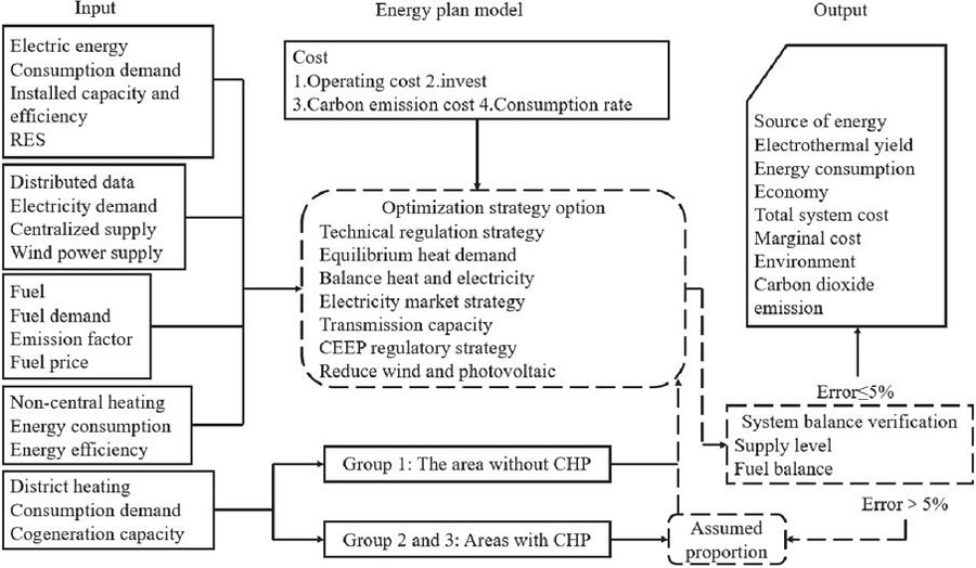
Figure 2 Technical route of scenario simulation of Energy PLAN model.
Energy PLAN is a model to determine the input and output, to obtain accurate simulation results, we must input accurate system parameters. Input data of Energy PLAN is divided into three categories: demand side, supply side, and cost side. Specific sources are summarized as follows:
(1) Demand side: The electricity demand is composed of the annual electricity consumption and distribution data of the whole society. Among them, the power consumption of the whole society is determined by the power balance table in the Statistical Yearbook 2021, and the distribution data comes from the power operation situation published by the Provincial Department of Industry and Information Technology and the regional distribution data in the 2020 China Electric Power Yearbook [13]. Taking into account the lack of central heating in the province, the heat demand is mainly composed of industrial heat and district heating, which is derived from the consumption of coal, natural gas, and biomass in the energy consumption table of the Statistical Yearbook 2021. Demand in the industrial and transport sectors is dominated by traditional fossil fuels (including coal, natural gas, gasoline, jet kerosene, diesel, and liquefied petroleum gas) and electric vehicle consumption. This part of the data comes from the energy consumption statistics of industrial enterprises and the comprehensive energy consumption statistics of major non-industrial energy-consuming units in Statistical Yearbook 2021 [14].
(2) Supply side: The power supply sector mainly includes thermal power and renewable energy, of which thermal power includes coal-fired power generation and biomass power generation, and renewable energy mainly includes onshore wind power, photovoltaic power generation, and hydropower. Input the installed capacity, efficiency, and power generation distribution of the above-mentioned power generation technology. The installed capacity data comes from the Provincial Energy Development Report 2020, and it is difficult to obtain the distribution data of renewable energy power generation. This part of the data integrates the power operation situation published by the provincial Department of Industry and Information Technology and the distribution data in the China model published by the official Energy PLAN [15]. The heat supply mainly includes the installed capacity, fuel consumption, and proportion of industrial cogeneration and heating boilers, which is derived from the “2021 China Urban Construction Statistical Yearbook”.
(3) Cost side: The cost is mainly divided into investment cost, operation and maintenance cost, fuel price, and carbon trading price. This part of the data directly refers to the cost model in the China model officially published by Energy PLAN.
2.3 Model Result Analysis
Based on the Energy PLAN model and the above data, it is possible to conduct a complete and comprehensive simulation of the energy system in 2020. This model will become a benchmark model and an important analysis model for subsequent research. By analyzing the consumption, supply, and balance of various departments in the system in 2020, the existing problems are explored to establish the direction for optimization [16]. In addition, the quantitative analysis of the economic, technical, and environmental performance of the basic model can provide an important basis for the selection of schemes. The simulation results include hourly distribution of electricity load, hourly distribution of power generation, hourly power balance, annual cost, and annual carbon emission, and the specific results are as follows.
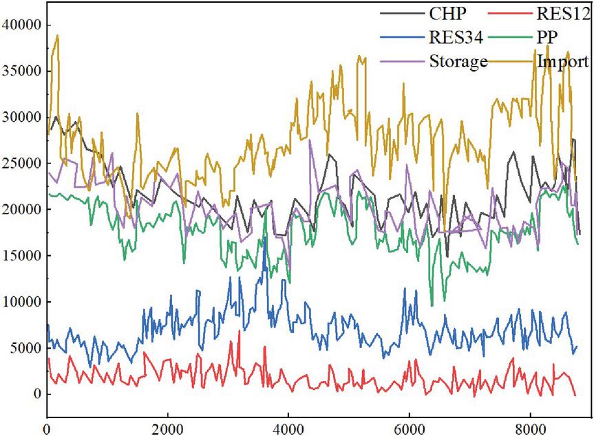
Figure 3 Hourly distribution of power supply.
In terms of power supply, as shown in Figure 3, thermal power (PP+) still bears more than 50% of the electricity load, and renewable energy generation shows great volatility, with sufficient supply in summer and obvious weakness in winter. As mentioned earlier, renewable energy in Hunan Province will account for 57% of the province’s total installed capacity in 2020, with hydropower reaching 17.1 million kilowatts. The limited regulation capacity of hydropower leads to more output in the summer flood season, while the supply capacity decreases significantly in the winter dry season. In recent years, the supply of thermal coal in Hunan Province has been insufficient and the price is high, and the benefit of coal-power investment is difficult to guarantee, and backward small units are constantly being eliminated [17]. Therefore, the installed thermal power capacity in the province gradually declined from 23.22 million kilowatts to less than 23 million kilowatts, which makes it difficult to meet the increasing electricity demand. In general, due to the special power supply composition of Hunan Province, renewable energy output fluctuates greatly, and the development of coal power is stagnant, so the total power is sufficient but insufficient power supply status.
The latest and most complete system data available in this paper is the data of 2020, so the energy system is simulated and verified based on the data of the 2020 energy system. The actual situation and simulation results of the main energy supply in 2020 are shown in Table 1. As shown in the table, the model has a small error in the simulation results of electricity and heat supply. Among them, conventional thermal power has the highest error rate, and its simulated value is smaller than the actual value, which may be partly due to the failure to consider grid transmission loss in this model [18]. On the other hand, the model’s simulation of thermal power is based on the strategy of mutual balance with cogeneration. In terms of thermal power output management, the balance strategy of cogeneration may be slightly different from that of conventional thermal power, thus causing errors in the results. However, the simulation error rate does not exceed 5%, which is considered to be in a reasonable range.
Table 1 Comparison of energy supply simulation results with actual data
| 2020 | Simulation | Difference | ||
| Item | Actual Data | Result | Value | Error Rate |
| Power supply | 110.53 | 109.44 | 1.09 | 0.99% |
| Conventional thermal power | 47.31 | 46.31 | 1 | 2.11% |
| CHP power generation | 19.13 | 20.01 | -0.88 | -4.60% |
| Water and electricity | 28.64 | 28.64 | 0 | 0.00% |
| Wind power generation | 11.42 | 11.42 | 0 | 0.00% |
| Photovoltaic power generation | 4.01 | 4.01 | 0 | 0.00% |
| Heat supply | 33.54 | 33.54 | 0 | 0.00% |
| Boiler heating g1 | 19.21 | 19.21 | 0 | 0.00% |
| Boiler heating g2 | 5.71 | 5.76 | -0.05 | -0.88% |
| CHP heating | 8.73 | 8.67 | 0.06 | 0.69% |
| Household energy supply | 47.67 | 46.94 | 0.73 | 1.53% |
In addition, biomass power generation, power supply from other provinces, and coal power generation are lower than the simulated value, mainly because of the impact of various factors such as epidemic prevention and control, at the beginning of the year, some enterprises stopped production, electricity demand is not strong, renewable energy consumption situation is grim, so the actual output of this kind of flexible adjustment power supply has declined relative to previous years. On the whole, the simulated values presented in the above table differ little from the actual values, with a maximum error of only 4.6%. In addition, considering that the epidemic has ended in China and the resumption of work and production is advancing steadily, it can be believed that during the “14th Five-Year PLAN” period, the high Energy demand and production obtained by the simulation of Energy PLAN will still be maintained, and the model has high accuracy.
3 Energy System Optimization Model Based on NSGA-II
3.1 Multi-time Scale Scheduling Model
According to the forecast curve of renewable energy output and load of the next day, the adjustable unit output plan and unit combination within 24h of the next day should be adjusted with 1 as the step size. Day-ahead scheduling model aims to minimize system operating costs and optimize environmental benefits, and takes electrical and thermal power flow constraints, unit climb constraints, and minimum start-stop time constraints as the main constraints, and its objective function expression is as follows [19].
| (1) | ||
| (2) |
T is the total number of periods in a scheduling cycle, and N is the total number of thermoelectric units.
(1) Power line power flow constraints
| (3) | ||
| (4) | ||
| (5) | ||
| (6) |
is the branch susceptance and is the branch reactance.
(2) Power balance constraints
| (7) | ||
| (8) |
Where: , and respectively represent the heat release of thermoelectric unit, GHP unit and EB during the period;
(3) Constraints on the active power output of the unit
| (9) | |
| (10) | |
| (11) | |
| (12) | |
| (13) | |
| (14) |
Where: and are respectively the pure condensate power generation output of thermoelectric unit i when the boiler output is limited up and down.
(4) Wind and light constraints
| (15) |
(5) Unit climbing constraints
| (16) |
(6) The minimum start-stop time constraint of thermoelectric units
| (17) |
(7) System rotation reserve constraints
| (18) |
(8) Wind power, photovoltaic unit output access power constraints
| (19) |
Due to the fluctuation and uncertainty of the output and load demand of wind power and photovoltaic units, the forecast curve in the previous 24-hour scheduling plan often has a certain error with the actual situation. To mitigate the impact of such forecasting errors on economic and environmental benefits, day-ahead scheduling plans need to be revised [20]. That is, at the current moment, according to the forecast value of the output and load of the wind turbine in the next few hours, the output of each turbine and the start-stop combination are planned again. In this chapter, the intra-day rolling adjustment period is set to 4 h, with 15 min as the adjustment step, that is, the period from the current period is the next adjustment period. To avoid frequent adjustments and improve the adjustment accuracy, the adjustment operation is only implemented when the first step of each cycle is long . The scheduling objectives of intra-day 4-hour rolling scheduling are as follows:
| (20) |
The relevant constraints are as follows.
(1) The minimum power on and off of the unit
| (21) |
(2) Wind and light constraints
| (22) |
3.2 NSGA-II Optimization Algorithm
NSGA algorithm was first proposed by scholars Srinivas and Deb in 1993. Although this algorithm has good robustness and optimization ability, with the increase of the number of optimization targets and the expansion of population size, it shows the shortcomings of high computational complexity and long solving time. Therefore, based on the NSGA algorithm, the NSGA-II algorithm was proposed in 2002, which is an improved version of the NSGA algorithm [21]. It can search and solve the target quickly, the solution range is wide, and the solution speed is relatively fast. On the one hand, the crowding degree and its comparison operator are proposed, so that individuals in the quasi-pareto domain can be evenly distributed in the whole Pareto domain to ensure population diversity. On the other hand, there is the combination of parent and child populations, which preserves the excellent individuals from the parents to the next generation. At the same time, through the stratified storage of individuals in the population, the purpose of preserving the best individuals and improving the population level is achieved. The improvement of the NSGA-II algorithm is mainly reflected in the following three aspects.
(1) A fast non-dominated sorting algorithm is added to the NSGA-II algorithm, which can greatly reduce the solving difficulty of the original algorithm. The algorithm classifies the population and greatly improves the solving speed.
Non-dominated sorting first calculates the objective function value of each individual. If at least one objective function value of an individual p is not less than that of another individual q, it is called P-dominated q. On the contrary, p is said to be dominated by q. If p dominates q, then q is added to the set Sp. If p is dominated by q, then np np+1. When np 0, it indicates that p is not dominated by any individual, so the domination level of individual p can be set as prank 1, and p can be added to the optimal front-end Fi. For each p present in front-end Fi, if Sp contains individual q (all individuals in Sp are known to be dominated by p), then nq nQ 1. When nq 0, it indicates that q is not dominated by other individuals, so the domination rank of individual q can be set to q i 1, and it will be added to the set Q.
(2) The NSGA-II algorithm introduces the elite selection strategy, which can protect the optimal individual from being eliminated to the greatest extent, to ensure the reliability and accuracy of optimization. In the selection process, the elite strategy combines the parent population and child population and stores population individuals in layers to ensure the depth and breadth of optimization [22].
(3) The crowding degree and the crowding degree operator are added to the NSGA-II algorithm, which can ensure the diversity of the solution set in the optimization process to the greatest extent. By calculating the crowding degree from the selected point to the daily scale function, and then comparing the crowding degree operator with the calculated crowding degree in the algorithm, the diversity of the population can be ensured and the Pareto solution set is evenly distributed.
Suppose that the initial distance between all individuals in a population with n individuals is 0, that is, set Fi(dj) 0, and j represents the j individual in the front-end Fi. Secondly, based on each objective function value, the individuals existing in front-end Fi are sorted, I sort (Fi, m). Let the distance of boundary entities be infinite, i.e. I(di) and I(dn) . The crowding distance of other individuals (k 2, …, n 1) is calculated according to the Euclidean distance formula. The calculation of crowding degree in the algorithm is shown in Equation (23).
| (23) |
In addition, the convergence index of the multi-objective optimization problem is usually represented by the average value of the minimum Euclidean distance, and the smaller the average value, the better the convergence, as calculated in Formula (24).
| (24) |
is usually used to represent the diversity of the solution set of a multi-objective optimization problem, and the smaller the value, the better the diversity is as shown in the calculation formula (25):
| (25) |
The basic flow chart of the NSGA-II algorithm is shown in Figure 4.
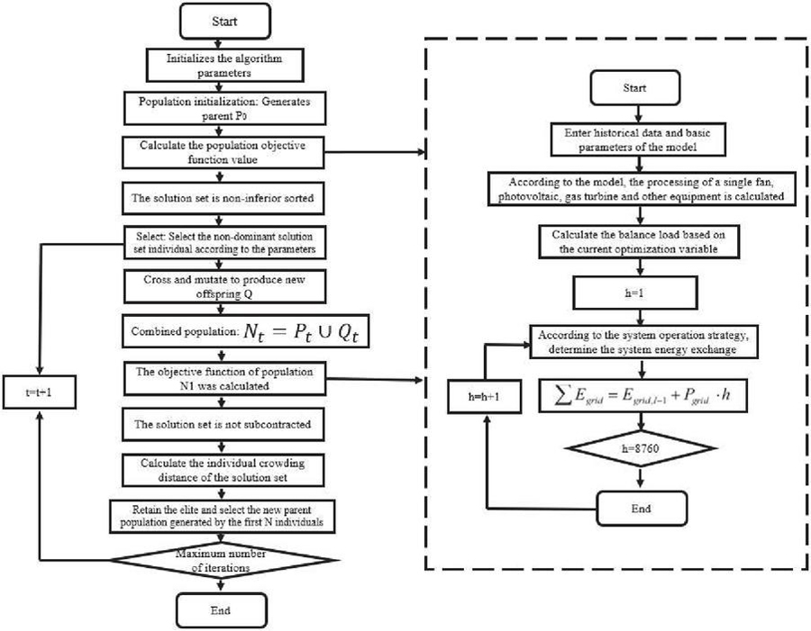
Figure 4 Flowchart of NSGA-II algorithm.
The solutions in the solution set X are first sorted according to the degree of fuzzy dominance from small to large so that the Pareto optimal frontier is closer to the ideal frontier [23]. On this basis, fuzzy set theory can be applied to further determine the optimal compromise solution. First, the fuzzy membership degree of the objective function satisfaction corresponding to each non-dominated solution is expressed as follows.
| (26) |
Secondly, the satisfaction of each non-dominant solution is standardized.
| (27) |
Finally, the non-dominant solution with the highest standardization satisfaction is the optimal compromise solution.
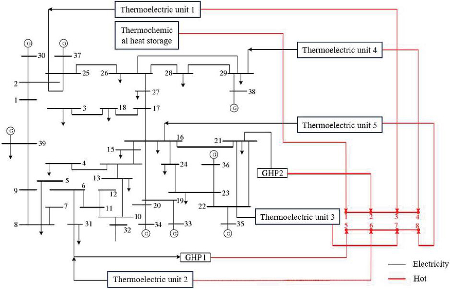
Figure 5 System network diagram.
3.3 Example Analysis
The system network is shown in Figure 5. The unit power investment cost, equipment service life, and the number limit or capacity limit of each equipment unit in CMIES are shown in Table 2.
Table 2 Parameters of energy equipment
| Life | Investment | Rated | Quantitative | Capacity | |
| Equipment | Span | Cost | Power | Restriction | Limitation |
| GT | 15 | 7700 | 500 | 6 | – |
| PV | 25 | 8700 | – | – | 30000 |
| GB | 20 | 420 | 150 | 200 | – |
| WHSP | 20 | 2200 | 75 | 400 | – |
| EC | 15 | 810 | 50 | 100 | – |
| AC | 15 | 670 | 200 | 25 | – |
| CFB | 20 | 4548 | 18750 | 4 | – |
| TFRR | 15 | 15000 | 670 | 5 | – |
| WHB | 15 | 200 | 100 | 300 | – |
| TS | 20 | 102 | – | – | 100000 |
This paper considers four scenarios in which associated energy and renewable energy participate in the configuration and sets the coal mine energy use scenario that does not consider the utilization of associated energy and renewable energy as the control scenario. Scenario 1 considers the comprehensive utilization of coal gangue, gas, and exhaust wind, while Scenario 2 considers the comprehensive utilization of photovoltaic power generation module, coal gangue, gas, and exhaust wind. The equipment configuration and Settings in each scenario are shown in Table 3.
Table 3 Configuration scenario settings
| Equipment | Contrast Scene | Scenario 1 | Scenario 2 |
| GT | |||
| PV | |||
| GB | |||
| WHSP | |||
| EC | |||
| AC | |||
| CFB | |||
| TFRR | |||
| WHB | |||
| TS |
Table 4 Energy system configuration in scenario 1
| Configuration Scheme | ||||||
| Equipment | S1 | S2 | S3 | S4 | S5 | Contrast Scene |
| GT | 3 | 3 | 3 | 3 | 3 | 0 |
| PV | 2.0 | 0 | 0 | 0 | 0 | 0 |
| GB | 2.84 | 21.4 | 21.3 | 0 | 8.9 | 25.8 |
| WHSP | 18.41 | 0 | 0 | 11.7 | 12.67 | 0 |
| EC | 3.7 | 0.5 | 0.9 | 0.9 | 3.9 | 4.6 |
| AC | 0.4 | 3.8 | 3.5 | 3.5 | 0.7 | 0 |
| CFB | 61 | 61 | 61 | 61 | 61 | 0 |
| TFRR | 3.34 | 3.38 | 3.35 | 3.36 | 3.36 | 0 |
| WHB | 0 | 0.5 | 10.7 | 10.8 | 0 | 0 |
| TS | 25 | 24 | 14 | 14 | 26 | 0 |
As shown in Table 4, the five schemes in scenario 1 are all configured with a coal stone generator set, a gas generator set, and an exhausted-air oxidation generator set to the maximum extent to provide electric energy to users and minimize the increase of carbon emission equivalent caused by air discharge of associated energy. The waste heat generated in the power generation process of the power generation unit can be converted into cold and heat energy through the waste heat boiler and absorption refrigerator to meet the diversified energy needs of the system. Scheme S2 and Scheme S3 are equipped with more gas boilers, and no water source heat pump is configured. Compared with scheme S2, scheme S3 is equipped with more waste heat boilers, so that the system waste heat can be preferentially used, and the gas boiler is used as the backup heat source, which reduces the carbon emission generated by the gas boiler. Scheme S1 and scheme S5 are equipped with a small amount of gas boilers, while scheme S4 is not equipped with gas boilers. These three schemes are equipped with more water-source heat pumps, thus reducing the consumption of natural gas. Such a configuration will reduce the carbon emission and economy of the system to a certain extent.
Table 5 Energy system configuration in scenario 2
| Configuration Scheme | ||||||
| Equipment | S1 | S2 | S3 | S4 | S5 | Contrast Scene |
| GT | 3 | 3 | 3 | 3 | 3 | 0 |
| PV | 30 | 30 | 24 | 3 | 30 | 0 |
| GB | 0 | 19.6 | 4.5 | 20.56 | 3.3 | 25.8 |
| WHSP | 3.16 | 1.876 | 2.631 | 1.426 | 1.575 | 0 |
| EC | 2.5 | 2.5 | 2.5 | 2.36 | 2.5 | 4.6 |
| AC | 1.8 | 1.9 | 1.8 | 2 | 1.8 | 0 |
| CFB | 61 | 61 | 61 | 61 | 61 | 0 |
| TFRR | 3.34 | 3.38 | 3.35 | 3.36 | 3.36 | 0 |
| WHB | 24.6 | 0 | 25.1 | 4.6 | 22.9 | 0 |
| TS | 40 | 35 | 38 | 19 | 39 | 0 |
As shown in Table 5, the coal gangue generator set, gas generator set, and exhaust air oxidation generator set are configured in the five schemes with maximum capacity. In this way, the associated energy of coal mines can be utilized to the maximum extent, the cost of purchasing electricity can be greatly reduced, and the carbon equivalent caused by energy waste and emptying can be reduced. The waste heat generated by the generator set in the power generation process can be further utilized and converted into cold/heat energy through the waste heat boiler and absorption chiller to meet the various energy needs of the system users. Option S4 is configured with a smaller capacity of PV equipment and the remaining options are configured with a maximum or slightly less maximum capacity of PV equipment. As CMIES increases the configuration of PV equipment, it will help reduce the cost of power purchases during the day. At the same time, it can also reduce the carbon emission equivalent caused by purchasing power from the grid, which can improve the economy of the system and improve the environmental benefits of the system to a certain extent. Scheme S1 does not consider the configuration of gas boilers and only considers the configuration of less water source heat pumps. However, with the addition of a larger capacity of heat storage equipment and a larger power waste heat boiler, the system will make more use of waste heat to meet the cold/heat requirements of the system under the configuration of this scheme. Unlike scheme S1, Scheme S3 is equipped with a small number of gas boilers and a slightly reduced heat storage capacity configuration. Scheme S2 and Scheme S4 are equipped with more gas boilers. The difference is that scheme S2 does not consider the use of waste heat boilers. Therefore, under scheme S2, the heat load of the system depends more on the supply of gas boilers.
Electrical energy is a cumulant, that is, the accumulation of power over some time, expressed in the form of discrete quantities.
| (28) |
The active power consumed by the corresponding A, B, and C three-phase power network is.
| (29) |
4 Result Analysis
To study the influence of the peak reversal effect of carbon emissions on the adjustment of energy structure, eight carbon emission scenarios (“L-L”, “L-M”, “M-L”, “M-M”, “M-M”, “M-H”, “H-L”, “H-M” and “H-H”) were used to examine the similarities and differences and changes of local production, input, and output of energy resources in the region under different scenarios. In general, the results of the lower bound submodel () do not change with the change in carbon emission scenarios. However, for the upper bound submodel () [24], the situation is different. Taking the total system cost during the planning period (see Figure 6) as an example, when the carbon emission scenario changes from “M-H” to “H-L”, that is, when the peak carbon emission gradually decreases, the total system cost will gradually increase. The main reason is that limited by the total amount of regional carbon emissions, more energy resources with lower carbon emission coefficients but higher costs (natural gas, etc.) will be used in the future [25].
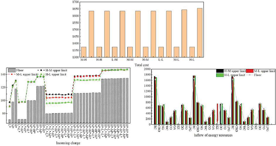
Figure 6 Eight cases of inflows.
The input of various energy resources (excluding heat) under the “H-M”, “M-L” and “H-L” carbon emission scenarios during the planning period is shown in Figure 6. As can be seen from Figure 6, under the same level of electricity demand, when the carbon emission scenario changes from “H-M” to “H-L”, the electricity inflow either gradually decline or almost stays the same. For example, when the power demand level is L*-L*-L*, the power inflow in the “H-M”, “M-L” and “H-L” scenarios is 106.02 10, 102.73 10, and 94.0 10 GWh, respectively. However, when the electricity demand level is H*-L*-L*, the electricity input is always 142.64 10 GWh, which does not change with the change of carbon emission scenario. In addition, relative to the other two scenarios, the “H-L” carbon emission scenario has the smallest electricity inflow. This is mainly due to the relatively high output of the missing generation technologies in this scenario. In addition, as shown in Figure 6, when the carbon emission scenario changes, only the inflow of raw coal and natural gas fluctuates, and the change trend is similar to that of the thermal production of coal-fired heating and gas combined cycle.
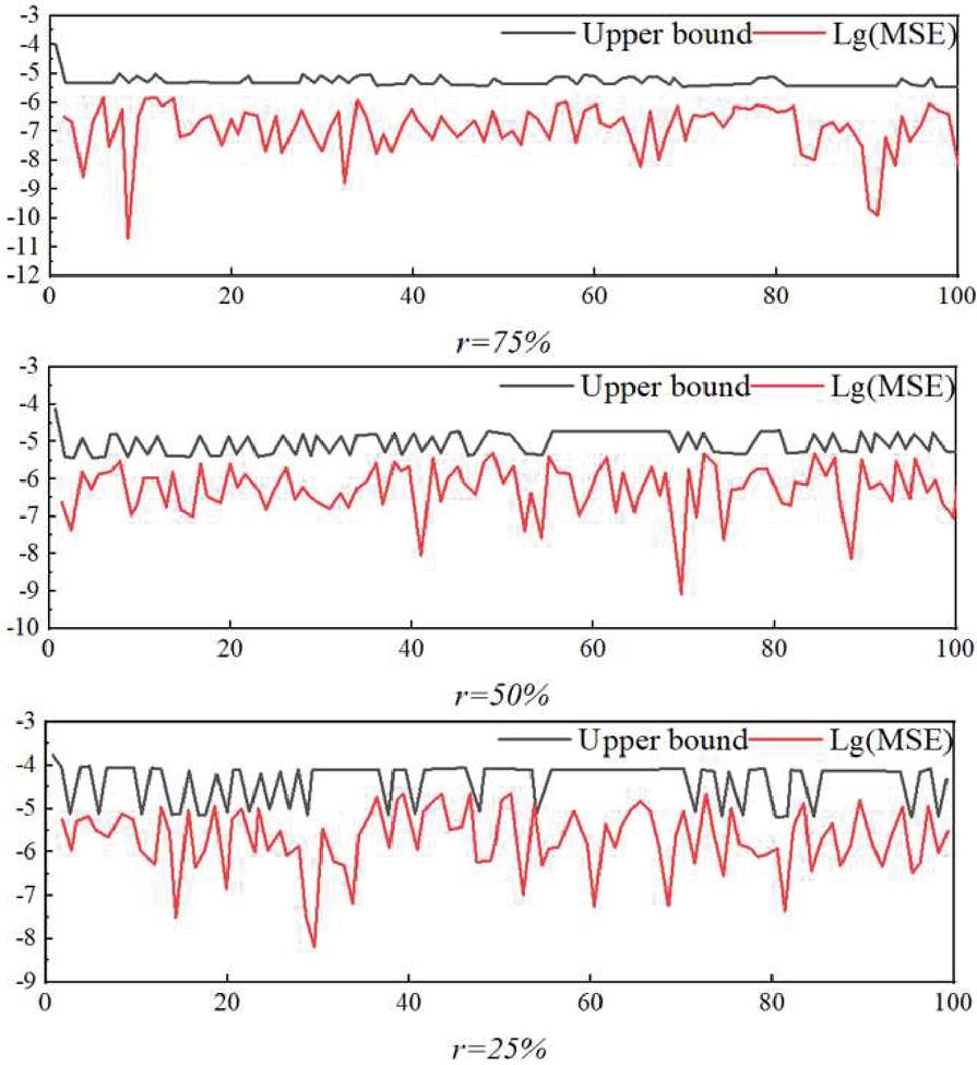
Figure 7 lg(MSE) and its upper bound.
Figure 7 shows lg(MSE) and its upper bound at different transmission rates. It can be seen that lg(MSE) at different transmission rates is always lower than its upper bound. In addition, with the decrease in the transmission rate, the error of the state estimation is increasing. When r 75%, the upper boundary voltage is maintained at about 5. When r 50%, the upper boundary voltage is maintained at about [5, 4.5]. When r 25%, the upper bound voltage is maintained at about [5, 4].
5 Conclusion
This paper analyzes and studies the intelligent Energy system based on the Energy PLAN model, and analyzes and validates the problems existing in the energy system from both theoretical and practical aspects. By comparing the actual data and the simulation results of Energy PLAN, the accuracy of the model is further verified, and the direction of energy structure reform is determined. By coupling the NSGA-II algorithm with the development model, a dual-objective multi-time scale scheduling model is established, which aims at the minimum operating cost and the best energy and environmental benefit coefficient. Specific conclusions are as follows.
1. The error of simulation results of the Energy PLAN model for power and heat supply is very small. Among them, conventional thermal power has the highest error rate, and its simulation value is smaller than the actual value, partly because the model does not consider the loss of grid transmission. On the other hand, the model’s simulation of thermal power is based on the strategy of mutual balance with cogeneration. In terms of thermal power output management, the balance strategy of cogeneration may be slightly different from that of conventional thermal power, thus causing errors in the results. However, the simulation error rate does not exceed 5%, which is considered to be in a reasonable range.
2. Scheme S1 does not consider the configuration of gas boilers and only considers the configuration of less water source heat pumps. However, with the addition of a larger capacity of heat storage equipment and a larger power waste heat boiler, the system will make more use of waste heat to meet the cold/heat requirements of the system under the configuration of this scheme. Unlike scheme S1, Scheme S3 is equipped with a small number of gas boilers and a slightly reduced heat storage capacity configuration. Scheme S2 and Scheme S4 are equipped with more gas boilers. The difference is that scheme S2 does not consider the use of waste heat boilers. Therefore, under scheme S2, the heat load of the system depends more on the supply of gas boilers.
3. When the power demand level is L*-L*-L*, the power input under the “H-M”, “M-L” and “H-L” scenarios is 106.02 10, 102.73 10 and 94.0 10 GWh, respectively. However, when the electricity demand level is H*-L*-L*, the electricity input is always 142.64 10 GWh, which does not change with the change of carbon emission scenario. In addition, relative to the other two scenarios, the “H-L” carbon emission scenario has the smallest electricity inflow. This is mainly due to the relatively high output of the missing generation technologies in this scenario. In addition, when the carbon emission scenario changes, only the inflow of raw coal and natural gas fluctuates, and the changing trend is similar to the changing trend of the thermal production of the coal-fired heating and gas combined cycle.
The objective function proposed in this paper is to optimize the whole system, and it can also be refined to the device level, so as to achieve the best performance of a single device unit. For example, the configuration of hybrid energy storage can be studied, and further research is expected to explore the above areas and improve the precision through algorithm improvement.
References
[1] Pohekar S D, Ramachandran M. Application of multi-criteria decision making to sustainable energy planning – A review[J]. Renewable and sustainable energy reviews, 2004, 8(4): 365–381.
[2] Hiremath R B, Shikha S, Ravindranath N H. Decentralized energy planning; modeling and application – a review[J]. Renewable and sustainable energy reviews, 2007, 11(5): 729–752.
[3] Yu Yang, Chen Dongyang, Wu Yuwei, et al. Battery energy storage Group Control Strategy for Reducing life loss in wind Power tracking Scheduling [J]. Electric Power Automation Equipment/Dianli Zidonghua Shebei, 2023, 43(3).
[4] Lu Quan, Zhang Jiawei, Zhang Na, et al. Coupling balance analysis model of the provincial electric-thermal integrated energy system with multiple flexible resources [J]. Automation of Power Systems, 2022.
[5] Li Chenxi, Liu Pei, Li Zheng. Urban energy system carbon reaches peak path optimization [J]. Journal of Tsinghua university (natural science edition), 2022 on conversion (4): 810–818. The DOI: 10.16511/j. carolcarrollnkiQHDXXB.2022.25.013.
[6] Xu Yan, Zhang Jianhao, Zhang Hui. Case study on location and capacity planning of Park integrated energy System containing cold, heat, electricity and gas [J]. Journal of Solar Energy, 2022, 43(1): 313.
[7] Cheng Jifeng, Yan Zheng, Li Mingjie. Optimization method of Surplus new energy power cross-province trading plan based on conditional value-at-risk and output forecasting [J]. High Voltage Technology, 2022, 48(2): 467–479.
[8] Duffield J S, Woodall B. Japan’s new basic energy plan[J]. Energy Policy, 2011, 39(6): 3741–3749.
[9] Løken E. Use of multicriteria decision analysis methods for energy planning problems[J]. Renewable and sustainable energy reviews, 2007, 11(7): 1584–1595.
[10] Kleinpeter M. Energy planning and policy[C]//Fuel and energy abstracts. 1995, 5(36): 382.
[11] Arnette A N. Renewable energy and carbon capture and sequestration for a reduced carbon energy plan: An optimization model[J]. Renewable and sustainable energy reviews, 2017, 70: 254–265.
[12] Brandoni C, Polonara F. The role of municipal energy planning in the regional energy-planning process[J]. Energy, 2012, 48(1): 323–338.
[13] Østergaard P A. Reviewing EnergyPLAN simulations and performance indicator applications in EnergyPLAN simulations[J]. Applied Energy, 2015, 154: 921–933.
[14] Debnath K B, Mourshed M. Forecasting methods in energy planning models[J]. Renewable and Sustainable Energy Reviews, 2018, 88: 297–325.
[15] Prasad R D, Bansal R C, Raturi A. Multi-faceted energy planning: A review[J]. Renewable and sustainable energy reviews, 2014, 38: 686–699.
[16] Mirakyan A, De Guio R. Integrated energy planning in cities and territories: A review of methods and tools[J]. Renewable and sustainable energy reviews, 2013, 22: 289–297.
[17] Mirakyan A, De Guio R. Modelling and uncertainties in integrated energy planning[J]. Renewable and Sustainable Energy Reviews, 2015, 46: 62–69.
[18] Lund H, Østergaard P A, Connolly D, et al. Smart energy and smart energy systems[J]. Energy, 2017, 137: 556–565.
[19] Yusoff Y, Ngadiman M S, Zain A M. Overview of NSGA-II for optimizing machining process parameters[J]. Procedia Engineering, 2011, 15: 3978–3983.
[20] Hamdani T M, Won J M, Alimi A M, et al. Multi-objective feature selection with NSGA II[C]//Adaptive and Natural Computing Algorithms: 8th International Conference, ICANNGA 2007, Warsaw, Poland, April 11–14, 2007, Proceedings, Part I 8. Springer Berlin Heidelberg, 2007: 240–247.
[21] DeCarolis J, Daly H, Dodds P, et al. Formalizing best practice for energy system optimization modelling[J]. Applied energy, 2017, 194: 184–198.
[22] Wang, Penghong, et al. “A Gaussian error correction multi-objective positioning model with NSGA-II.” Concurrency and Computation: Practice and Experience 32.5 (2020): e5464.
[23] Hansen K, Mathiesen B V, Skov I R. Full energy system transition towards 100% renewable energy in Germany in 2050[J]. Renewable and Sustainable Energy Reviews, 2019, 102: 1–13.
[24] Terrados J, Almonacid G, PeRez-Higueras P. Proposal for a combined methodology for renewable energy planning. Application to a Spanish region[J]. Renewable and sustainable energy reviews, 2009, 13(8): 2022–2030.
[25] Wu C B, Huang G H, Liu Z P, et al. Scenario analysis of carbon emissions’ anti-driving effect on Qingdao’s energy structure adjustment with an optimization model, Part II: Energy system planning and management[J]. Journal of environmental management, 2017, 188: 120–136.
Biographies
Ce Peng Graduated from Wuhan University with a bachelor’s degree, majoring in Electrical Engineering and Automation. After graduation, I worked at Guangdong Power Grid Co., Ltd., with a main research focus on electricity. The current professional title is Senior Engineer.
FanQin Zeng Graduated from South China University of Technology with a master’s degree in electrical engineering. After graduation, I worked at the Metrology Center of Guangdong Power Grid Co., Ltd., with a main research focus on electricity.
Youpeng Huang Graduated from Huazhong University of Science and Technology with a master’s degree in Electrical Engineering. After graduation, I worked at the Metrology Center of Guangdong Power Grid Co., Ltd. My main research direction is energy metering. The current professional title is Senior Engineer.
Zhaopeng Huang Graduated from Sun Yat sen University with a bachelor’s degree, majoring in computer software. After graduation, I worked at Foshan Power Supply Bureau of Guangdong Power Grid Corporation., with a main research focus on electricity. The current professional title is Engineer.
Xinming Mao Graduated from Southwest Jiaotong University with a master’s degree, majoring in Computer Application Technology. After graduation, I worked at China Energy Engineering Group Guangzhou Electric Power Design Institute Co.,Ltd, with a main research focus on electricity. The current professional title is Senior Engineer.
Strategic Planning for Energy and the Environment, Vol. 43_3, 715–740.
doi: 10.13052/spee1048-5236.43310
© 2024 River Publishers