Multisource Data-Driven Carbon Price Composite Forecasting Model: Based on Feature Selection and Multiscale Prediction Strategy
Shaohui Zou and Jing Zhang*
School of Management, Xi’an University of Science and Technology, Xi’an 710054, China
E-mail: 21202097039@stu.xust.edu.cn
*Corresponding Author
Received 15 March 2024; Accepted 04 April 2024
Abstract
Accurate prediction of carbon trading prices is crucial for guiding investors to make informed decisions and assisting governments in formulating scientific carbon trading policies. This paper introduces a multisource data-driven carbon price composite forecasting model, aimed at enhancing prediction accuracy through advanced data processing and analysis methods. The model initially employs a secondary decomposition strategy, including Complete Ensemble Empirical Mode Decomposition with Adaptive Noise (CEEMDAN) and Variational Mode Decomposition (VMD) methods, to decompose the original data series into three sub-sequences of different frequencies. Subsequently, it utilizes the Partial Autocorrelation Function (PACF) and Random Forest algorithm for feature selection to determine the input variables for different frequency sequences and conducts in-depth analysis and selection of influencing factors, including unstructured data. Furthermore, the model employs a multiscale forecasting strategy, combining Particle Swarm Optimization (PSO) enhanced Bidirectional Long Short-Term Memory (BiLSTM) and Extreme Gradient Boosting (XGBoost) models, along with the Autoregressive Integrated Moving Average (ARIMA) method, to predict based on the characteristics of different frequency components. Finally, the forecasts are integrated using PSO-BiLSTM to form a comprehensive forecast. Notably, given the high correlation between the trend series and influencing factor variables, the model jointly predicts them. A case study based on the Guangdong carbon market in China demonstrates that the proposed composite forecasting model outperforms other benchmark models, with Root Mean Square Error (RMSE), Mean Absolute Error (MAE), and Mean Absolute Percentage Error (MAPE) values of 0.4009, 0.2699, and 0.5183%, respectively. This forecasting model provides an effective tool for predicting and analyzing carbon price fluctuations, offering new insights for precise carbon market price predictions.
Keywords: Carbon price forecasting, second decomposition, feature selection, unstructured data, influencing factors, bidirectional long short-term memory network, extreme gradient boosting, particle swarm optimization.
List of Notations and Abbreviations
ARIMA: Autoregressive Integrated Moving Average
ANN: Artificial Neural Network
BiLSTM: Bidirectional Long Short-Term Memory
CEEMD: Complementary Ensemble Empirical Mode Decomposition
CEEMDAN: Complete Ensemble Empirical Mode Decomposition with Adaptive Noise
EMD: Empirical Mode Decomposition
EEMD: Ensemble Empirical Mode Decomposition
IMF: Intrinsic Mode Function
IMF1: The first Intrinsic Mode Function by decomposition
LSTM: Long Short-Term Memory
PSO: Particle Swarm Optimization
PSO-XGBoost: eXtreme Gradient Boosting for parameter optimization using particle swarm optimization algorithm
PSO-BiLSTM: Bidirectional Long Short-Term Memory for parameter optimization using particle swarm optimization algorithm
PACF: Partial AutoCorrelation Function
RF: Random Forest
SE: Sample Entropy
VMD: Variational Mode Decomposition
XGBoost: eXtreme Gradient Boosting
1 Introduction
With the rapid development of the global economy, environmental and energy issues have become increasingly prominent, with greenhouse gas emissions posing a serious threat to sustainable human development. Historical experience has shown that relying solely on mandatory emission reduction requirements or voluntary emissions reduction by economic entities makes it difficult to achieve emission reduction goals. The emissions trading market for carbon dioxide stands as an efficient avenue to achieve economic emission reduction within a market-driven framework. As a core element of the carbon market, accurately predicting carbon trading market prices, also known as “carbon prices,” can guide carbon market participants and policymakers in making effective decisions, foster market stability, and propel low-carbon economic growth. Therefore, improving the precision of carbon price prediction has emerged as a vital focus in academic and industry circles.
In recent years, scholars have proposed numerous prediction models to enhance carbon price precision. Currently, prevalent carbon price prediction methods can be broadly categorized into three types: traditional statistical analysis methods, artificial intelligence methods, and combination forecasting methods. The traditional statistical analysis methods have the advantages of simplicity and computational efficiency [1–4]. However, carbon price data is influenced by multiple factors such as energy prices, policy changes, and weather variations, making it challenging for traditional statistical and econometric methods to reflect the data’s nonlinear characteristics fully. The development of artificial intelligence algorithms have provided new directions for carbon price prediction. They can induce and summarize complex nonlinear mapping relationships through statistical analysis of historical data, effectively capturing the hidden nonlinear patterns in carbon market prices [5]. These models exhibit excellent performance in learning, generalization, computational speed, and prediction accuracy for carbon price series [6], making them widely applied in carbon price forecasting [7–9].
Combination models aim to gather the advantages of various models, avoid their limitations, and improve the predictive performance of each model, thereby maximizing the capture of nonlinear features in carbon price data. As a result, AI-based combination forecasting models have become the most favored method among scholars in the current research on carbon price prediction. Among these models, the decomposition-ensemble combination forecasting model, which combines decomposition and prediction methods, is a commonly used approach in time series forecasting. This method decomposes the time series, reducing noise while expanding the sample size, thus enabling the extraction of more effective features. It has been extensively applied in forecasting research across various domains, such as energy prices [10, 11], stock price indices [12], soil temperature [13], electricity load [14], wind speed [15], and more. Since carbon price data is a complex time series with noise contamination, the Combined prediction model based on the decomposition-ensemble framework has also emerged as one of the mainstream prediction methods in carbon price research. Zhu et al. [16] utilized Empirical Mode Decomposition (EMD) and hierarchical clustering methods to decompose and reconstruct the EU ETS carbon futures prices. They obtained eight Intrinsic Mode Functions (IMFs) and one residual sequence through decomposition and then used hierarchical clustering to reconstruct them into high-frequency, low-frequency, and trend components. While simplifying the complex series, this approach revealed the short, medium, and long-term fluctuations and trends in the carbon market. Sun and Li [17] proposed an ensemble-driven carbon price prediction model based on Complementary Ensemble Empirical Mode Decomposition (CEEMD). Firstly, they employed CEEMD to decompose the original carbon price series into a set of simple modal components. Then, they selected time lag features from the components using the Partial Autocorrelation Function (PACF) and used these features as inputs for multiple Long Short-Term Memory (LSTM) models to obtain predictions for each component. Finally, they integrated the results using the inverse CEEMD method to derive the ultimate carbon price predictions. The findings demonstrated that compared to single LSTM models and other traditional ANN models, the proposed model exhibited higher prediction accuracy. The practice has confirmed the superiority of the decomposition-ensemble framework-based prediction model within the realm of carbon price prediction [6, 18].
In the realm of decomposition and ensemble forecasting methods, limitations still persist. Zhou et al. [19] developed a carbon price forecasting model based on the Complete Ensemble Empirical Mode Decomposition with Adaptive Noise (CEEMDAN) approach and LSTM. Empirical analysis revealed that CEEMDAN is not ideal for decomposing high-frequency components such as the first IMF (IMF1), resulting in decompositions with high volatility and irregularity, which may adversely affect the overall prediction accuracy. Subsequent improvements and studies have shown that a secondary decomposition method based on Variational Mode Decomposition (VMD) can effectively decompose highly volatile high-frequency sequences like IMF1. Some scholars also reached similar conclusions in their research, confirming the positive effect of using VMD for secondary decomposition in predictions. Sun and Huang [20] proposed a new carbon price prediction model that, based on the decomposition-ensemble forecasting framework, utilized VMD for the secondary decomposition of IMF1 obtained through EMD decomposition. In simulation research on the carbon market in Hubei, China, their proposed model improved R by 43.9% and reduced MAPE and RMSE by 1.5% and 43.0%, respectively, compared to the model without VMD. Similarly, Zhou and Wang [21] also introduced a combination forecasting model that utilized VMD for the secondary decomposition of the strongest volatile IMF1 after the CEEMDAN decomposition of the original sequence. Compared to the forecasting model without secondary decomposition, this model improved R, MAPE, and RMSE by 2.5%, 55.6%, and 55.2%, respectively, enhancing the predictive precision. It demonstrates that the secondary decomposition strategy based on CEEMDAN-VMD can effectively improve the accuracy of the decomposition-ensemble prediction model.
In addition, many studies on carbon price prediction are confined to the application of historical data to build prediction models. Although historical data contains important characteristics of carbon price changes, its prediction results are often lagging behind. Moreover, carbon price volatility is influenced by a variety of factors, and the analysis and study of these factors are equally important for carbon price prediction. With the increasingly developed internet environment, the use of search engines has become more frequent, leading to the widespread presence of unstructured data. Studies have indicated that incorporating unstructured data with a certain predictive power into the forecasting process can provide a wealth of valid information for time series prediction, thereby improving the accuracy of forecasts [22, 23]. Therefore, it is necessary to explore the effective information provided by unstructured data to enhance the accuracy of predictions. Currently, few studies have attempted to combine unstructured data for predicting carbon trading prices.
The complexity of the carbon trading system endows the carbon price time series with characteristics such as nonlinearity and high noise levels. While adding unstructured data and influential factors can provide richer information for carbon price prediction, it also increases the complexity of the data, potentially introducing more redundant or irrelevant features into the model input. These redundant features not only increase the training time but can also reduce the accuracy of predictions. Feature selection, which identifies the best input features highly correlated with the predictive variable [24], is a crucial step in developing artificial neural network prediction models. Therefore, feature selection methods should be employed in carbon price forecasting to achieve better predictive performance.
From the research mentioned above, it can be understood that: First, the “decomposition-ensemble” forecasting framework exhibits excellent predictive capabilities in the field of carbon price forecasting. However, a single decomposition process yields poor results for the decomposition of highly volatile IMF components. Relevant studies have shown that a secondary decomposition strategy based on VMD can effectively address this issue. Secondly, few studies have utilized multiple methods to predict based on the characteristics of the subsequences of different frequencies obtained from the decomposition. Moreover, carbon price forecasting studies that introduce influencing factor data rarely consider unstructured data such as web search indexes.
Therefore, this paper introduces unstructured data and other external influencing factors, and based on multi-source data, proposes a combined prediction model that combines quadratic decomposition strategy, feature selection method, and multi-scale integrated prediction strategy including Bidirectional Long Short-Term Memory (BiLSTM), eXtreme Gradient Boosting (XGBoost), and Autoregressive Integrated Moving Average (ARIMA) models to predict features of different frequency components. Among them, the PSO algorithm is used to optimize the parameters of BiLSTM (PSO-BiLSTM) and XGBoost (PSO-XGBoost) models with large parameter adjustment space, so as to improve the accuracy of carbon price prediction. The innovations of this paper can be summarized as follows:
(1) This paper presents a novel composite forecasting model for carbon prices. This model integrates a secondary decomposition strategy, feature selection methods, intelligent optimization algorithms, artificial intelligence algorithms such as BiLSTM and XGBoost, and the traditional statistical method ARIMA, aiming to maximize the strengths of each model while minimizing the bias or uncertainty that any single model might introduce.
(2) A multiscale forecasting strategy is proposed, selecting appropriate methods to predict based on the characteristics of subsequences at different frequencies. Herein, the PSO-BiLSTM model is used for predicting high-frequency sequences, PSO-XGBoost for trend sequences and influencing factors, and the ARIMA method for low-frequency sequences. Subsequently, an ensemble of the predictions from the above processes through PSO-BiLSTM is performed to obtain the final forecasting result.
(3) The study employs a multi-source data fusion strategy for forecasting, conducting an in-depth analysis and comprehensive consideration of carbon prices’ historical data, unstructured data, and other key external influencing factors. This holistic data integration approach enables a more precise capture and understanding of the complex dynamics affecting carbon price fluctuations, providing solid data support for improving the model’s forecasting accuracy.
(4) A feature selection mechanism has been established, conducting feature selection in two phases for the influencing factors of carbon prices and the internal features, i.e., historical carbon price data, to avoid the interference of redundant features and help the model effectively capture key features.
(5) Actual carbon price data were collected to establish nine comparison models and three evaluation indicators. A case study based on the Guangdong carbon trading pilot demonstrates that the proposed model exhibits higher forecasting accuracy and universality.
The subsequent sections of this study are structured as follows: Section 2 primarily elucidates the foundational principles underpinning the employed methodologies. Section 3 mainly describes the construction process of the proposed combination forecasting model. Sections 4 and 5 primarily presents the data selection, feature analysis, evaluation indicators, empirical research process, and result analysis. Section 6 mainly expounds upon the central discoveries of this paper and outlines avenues for future exploration.
2 Method
2.1 CEEMDAN
The CEEMDAN (Complete Ensemble Empirical Mode Decomposition with Adaptive Noise) method is an advanced signal processing technique used for analyzing time series data. It adaptively decomposes a time series into IMF components, ranging from high to low frequency with different time scale characteristics, as well as a residue (Res) component. This method is particularly suitable for handling nonlinear and non-stationary time series of carbon prices. The decomposition process of CEEMDAN is as follows:
Let be the original data sequence, be the order modal component generated by the EMD algorithm, and define as the order intrinsic mode component sequence generated by the CEEMDAN algorithm. Let be the Gaussian white noise sequence added for the iteration, be the adaptive Gaussian white noise weight coefficient, and represent different time points. The basic implementation process of this algorithm is as follows:
(1) Add Gaussian white noise sequences with zero means times to the original time series , and construct a sequence containing experimental decompositions:
| (1) |
(2) Perform an Empirical Mode Decomposition (EMD) on , and denote the resulting first-order Intrinsic Mode Functions (IMFs) as . The first IMF obtained from the decomposition is:
| (2) |
At this moment, the only first-order residual sequence is:
| (3) |
(3) Add adaptive Gaussian white noise to the residual sequence , and use it as the new sequence for EMD decomposition. Then, calculate the second-order IMF and the residual sequence of CEEMDAN:
| (4) | |
| (5) |
Where represents the first IMF obtained through EMD.
(4) And so on, the residual sequence and the IMF of the order are obtained as follows:
| (6) | |
| (7) |
where represents the IMF obtained through EMD.
(5) When the obtained residual sequence cannot be further decomposed and the number of extreme points does not exceed two, the CEEMDAN decomposition is completed. At this point, the original signal is decomposed into several IMFs and one residual sequence, and the final residual sequence satisfies:
| (8) |
If the final decomposition results in modal components, then the original carbon price sequence can be represented as:
| (9) |
2.2 VMD
The Variational Mode Decomposition (VMD) method, proposed by Dragomiretskiy and Zosso [25], is a non-recursive signal processing technique specifically designed to address the issue of modal separation in complex signals. VMD is capable of adaptively decomposing a complex signal into a series of band-limited Intrinsic Mode Functions (IMFs), with each IMF capturing a principal frequency component of the signal, thereby facilitating easier analysis and processing of the decomposed components. Unlike the classical Empirical Mode Decomposition (EMD) and its enhanced version, CEEMDAN, VMD employs a variational approach to identify and extract individual modal components within a signal. It exhibits robust resistance to noise and can overcome problems related to mode mixing and sensitivity to noise.
(1) Construct a variational optimization model based on the objective of the variational problem:
| (10) |
Where represent the number of IMFs obtained from the decomposition. and denote the set of all modal signals and their central frequencies from the decomposition. represents the partial derivative operator with respect to . stands for the Dirac function, and denotes the convolution operator.
(2) To solve the above optimization problem, we introduce a quadratic penalty factor and Lagrange multipliers , transforming the constrained variational problem into an unconstrained variational problem. The constructed augmented Lagrangian function is as follows:
| (11) |
(3) Initialize , , , and . Use , , and to represent the Fourier transforms of , , and , respectively. is the tolerance for noise. In the Fourier transform domain, update , , and using the Alternating Direction Method of Multipliers (ADMM) algorithm to search for saddle points in formula (2.2). The update equations are as follows:
| (12) | |
| (13) | |
| (14) |
(4) The updates will be stopped When the stopping condition in formula (15) is satisfied.
| (15) |
2.3 XGBoost
XGBoost (eXtreme Gradient Boosting) is a powerful machine learning algorithm that is particularly effective for regression and classification problems. It is built on a gradient boosting framework and utilizes decision trees as its base learners. Boosting, an ensemble learning method, iteratively trains weak learners (e.g., decision trees), focusing on samples misclassified by the model in previous iterations and assigning them higher weights to correct the errors, culminating in a strong model. As a tree-based model, XGBoost excels in handling and capturing nonlinear relationships and complex interactions between features. This gives it a distinct advantage in analyzing datasets with multiple influencing factors. Therefore, this study chooses to employ XGBoost for predicting and analyzing carbon price influencing factor data, leveraging the model’s advanced computational efficiency and flexibility, as well as its robust performance in dealing with diverse and complex data structures. For details on XGBoost’s specific computational process, refer to the papers by its creator, Tianqi Chen, et al. [26].
XGBoost has several parameters, and because some model parameters significantly impact the results, it is necessary to optimize key parameters. This study optimizes crucial parameters of XGBoost, such as the learning rate, number of trees, tree depth, sample sampling rate, minimum child weight, and the intensity of decision tree pruning, using the Particle Swarm Optimization (PSO) algorithm. This is done to maximize the predictive capability of the XGBoost model and enhance prediction accuracy.
2.4 BiLSTM
Long Short-Term Memory (LSTM) networks are a variant of Recurrent Neural Networks (RNNs). They address the inability of RNNs to handle long-term dependencies, with their core being the use of memory cells to retain long-term historical information and the adoption of specially designed gate mechanisms (input gate, forget gate, and output gate) to select information to be retained or forgotten. The input gate, comprised of a sigmoid neural network layer, controls the entrance of new information; the forget gate, formed by a sigmoid neural network layer and a pointwise multiplication operation, manages the retention and forgetting of information; the output gate works together with a tanh activation function and a pointwise multiplication operation to transfer the cell state and input to the output.
In processing time-series data, unidirectional LSTM network structures have shown good predictive performance for nonlinear time series. However, they can only capture information from previous nodes and are unable to utilize the influence of subsequent node information on the current node. Bidirectional LSTM (BiLSTM) employs two LSTM networks in opposite directions, enabling the utilization of state information from both previous and subsequent nodes to enhance prediction accuracy. The computation of BiLSTM is divided into forward and backward calculations, where the horizontal axis represents the bidirectional flow of the time series, and the vertical axis indicates the unidirectional flow of information from the input layer to the hidden layer and from the hidden layer to the output layer. The main computational process of BiLSTM can be represented by Equation (16):
| (16) |
Where and represent the outputs of the hidden layer from both the forward and backward LSTM networks at time , respectively. and denote the operations of the forward and backward LSTM, while and are the matrices containing the weights for the forward and backward LSTM layers. is the bias term of the output layer.
In this paper, PSO algorithm is used to optimize five parameters of BiLSTM’s neural network, including the number of layers, the number of neurons per layer, the number of samples per training, the learning rate and Dropout rate, in order to improve its prediction ability in the carbon price prediction task and obtain higher prediction accuracy.
2.5 ARIMA
The Autoregressive Integrated Moving Average (ARIMA) model is a classic method for analyzing and forecasting time series data. The basic form of an ARIMA model is denoted as , where is the Integrated order, representing the number of times a difference is made to make the time series stationary. is an AutoRegressive order and represents the observations for the previous periods considered in the model. is the order of the Moving Average, which represents the prediction error for the previous periods considered in the model. Its mathematical expression is
| (17) |
Where is time series data; is the Lag operator, which represents the lag value of the time series. is the parameter of the autoregressive (AR) term; is the parameter of the moving average (MA) term; is the error term, which is usually assumed to be white noise.
2.6 PSO
The Particle Swarm Optimization (PSO) algorithm is a population-based optimization technique that simulates the social cooperation mechanism of bird flocking behavior for global searching, demonstrating significant effectiveness in solving complex optimization problems. Its main idea involves finding the optimal solution through cooperation and information sharing among individuals within the population. Compared to conventional genetic algorithms, the standard PSO algorithm simplifies the process by reducing operations such as crossover and mutation, offering a simpler structure and faster convergence.
When solving optimization problems, the PSO algorithm updates particle velocity and position by tracking both the individual best particle and the best particle across the entire population. This process can be delineated as follows: In a -dimensional search space, there is a particle swarm consisting of randomly initialized particles. At the iteration, the position and velocity of the particle in the dimension are denoted as and , respectively. Each particle continuously updates its position and velocity to explore the entire state space by tracking its individual best solution and the global best solution found by the entire population. The ultimate goal is to gradually search for the optimal position, i.e., the optimal solution. The updates of velocity and position follow formulas (18) and (19).
| (18) | |
| (19) |
Where represents the inertia weight, and are the learning factors; and are uniformly distributed random numbers within the range [0,1].
2.7 PACF
The Partial Auto Correlation Function (PACF) is used to analyze the partial auto-correlation relationships at various lag orders within time series data. It describes the auto-correlation of a specific lag order after eliminating the influence of other lag orders. PACF is often utilized to guide model selection and the determination of input features in time series forecasting, helping identify which lag orders are significant for modeling and prediction. By analyzing the PACF, a better understanding of the structure within time series data can be achieved, providing guidance for establishing accurate forecasting models. For a time series , the PACF at lag can typically be represented as :
| (20) |
Where, represents the value of time series at time point; and are the predicted values of and ; is the correlation coefficient.
2.8 RF
Random Forest (RF) is a classic machine learning algorithm introduced by Leo Breiman in 2001. This algorithm combines a weak model – Classification and Regression Trees (CART) – with the Bagging method and the Random Subspace Method (RSM), incorporating both Bootstrap Aggregating (Bagging) techniques and RSM technology. In RF, CART trees are constructed by randomly selecting a subset of samples from the dataset with replacement, while the samples not selected are referred to as Out-Of-Bag (OOB) samples. These OOB samples are utilized for internal validation of the model, and the final output of the model is determined through a voting mechanism.
This research employs the feature importance evaluation functionality within RF to filter the input features for high-frequency sequences. The principle involves artificially altering the values of features (by adding white noise) to compute the Out-Of-Bag (OOB) error on the model training set. Since the OOB error serves as an unbiased estimate of the model’s generalization capability, a greater increase in error signifies a larger impact of the variable. Consequently, model features with minimal relevance to the prediction variable are discarded, thereby enhancing the accuracy of the predictions.
The original OOB error of the RF model is denoted as , and the OOB error of the model after adding noise to the sample feature is denoted as . The importance of feature can be calculated using Equation (21):
| (21) |
2.9 MIC
The Maximal Information Coefficient (MIC) method, proposed by Reshef et al., is a correlation analysis method based on information theory. For any given pair of variables and , the mutual information (MI) between them is defined as the expected value of the logarithmic ratio of their joint distribution to the marginal distributions, reflecting the amount of mutual information between the variables. MIC is determined by evaluating the maximum MI across different grid partitions, thus providing a powerful tool for detecting and quantifying the correlation between variables. The MI between variables and can be defined as:
| (22) |
Where, denotes the joint probability density function for variables and , and and respectively denote the marginal probability density functions for and .
2.10 Pearson Correlation Coefficient
The Pearson correlation coefficient is a statistical measure used to evaluate the strength and direction of the linear relationship between two variables. In feature selection, this method can be employed to identify features that are highly correlated with the target variable. Its value ranges from [1, 1], where: 1 signifies a perfect positive correlation, implying that as one variable rises, the other variable also increases proportionally. 1 signifies a perfect negative correlation, implying that as one variable rises, the other decreases proportionally. 0 signifies the absence of a linear relationship. For two variables and , the calculation formula for the Pearson correlation coefficient is as follows:
| (23) |
Where, and are the observed values of the two variables; and are the average values of the two variables.
When used for correlation analysis involving multiple variables, Pearson typically generates a correlation matrix, where each element in the matrix represents the Pearson correlation coefficient between two variables. The correlation matrix is extensively applied in areas like multivariate data analysis, feature selection, and factor analysis.
2.11 SE
Sample Entropy (SE) constitutes a technique devised by Richman and Moorman to gauge the intricacy of time series, and it represents an improvement over approximate entropy. In contrast to the latter, the computation of SE remains unaffected by data length and exhibits better robustness and consistency. When is a finite value, the definition of sample entropy can be expressed as follows:
| (24) |
Where represents the length of the input signal, represents the dimension, and represents the tolerance of similarity.
3 The Construction Process of the Proposed Model
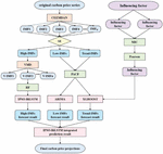
The carbon price combination forecasting model proposed in this paper refers to the combined forecasting framework based on VMD secondary decomposition proposed by Zhou et al. [19]. The modeling process is illustrated in Figure 1, and steps for modeling are outlined as follows.
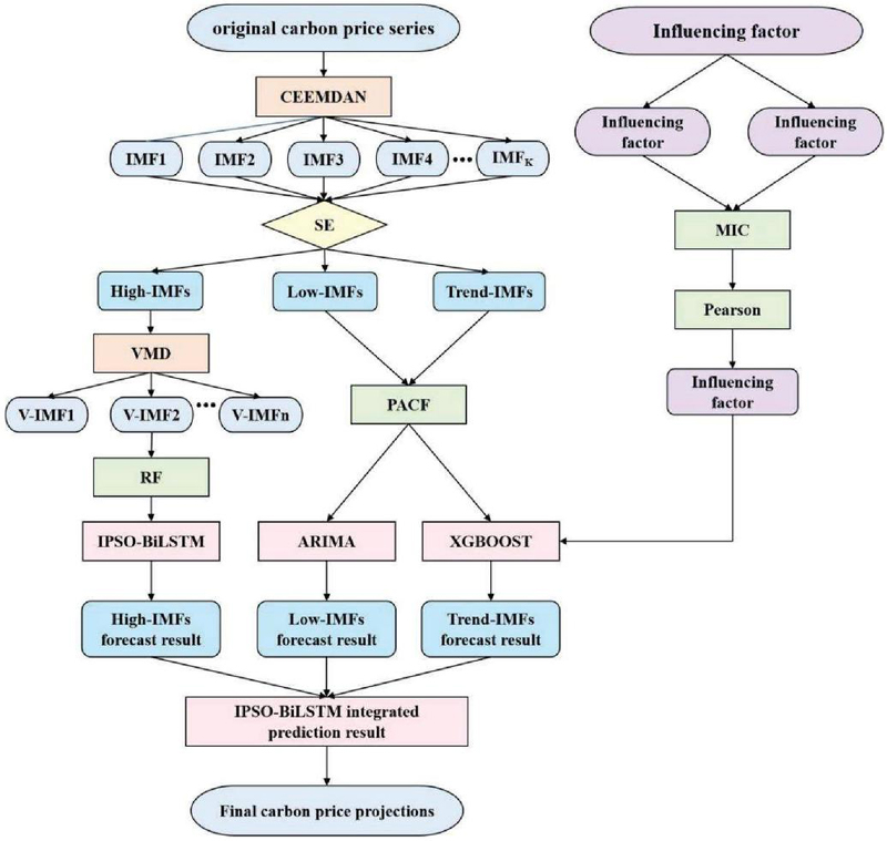
Figure 1 Flow chart of the mode.
3.1 Secondary Decomposition
(1) The original carbon price series is processed using the CEEMDAN method, decomposing it into several Intrinsic Mode Functions (IMFs).
(2) Based on the calculation results of the Shannon Entropy (SE) values for each component series, all IMFs are classified into high-frequency, low-frequency, and trend components, which are then aggregated to form three new component series: the high-frequency, the low-frequency, and the trend series.
(3) The VMD method is applied for secondary decomposition, resulting in several new modal components.
3.2 Feature Selection
To obtain the optimal input features, this paper establishes a two-stage feature selection mechanism. In the first stage, the PACF and RF are used for feature selection on the high-frequency, low-frequency, and trend series, obtaining input variables of internal features. In the second stage, influence factors are ranked and filtered by calculating their MIC and Pearson correlation coefficient values. The specific process is as follows:
(1) First Stage – Internal Feature Selection
For the low-frequency and trend series, solve for PACF results up to the 30th order, selecting lag orders that exceed the 95% confidence interval as input variables for the low-frequency and trend series, respectively. The importance of variables is ranked using the RF algorithm, and the top five series are selected as input variables for the high-frequency series.
(2) Second Stage – External Feature Selection
Conduct MIC analysis on the selected structured and unstructured influence factor variables and the original series, choosing influence factors with MIC values greater than 0.5. Afterwards, calculate the Pearson correlation coefficient values for the selected influence factors, and those with values greater than 0.5, indicating a strong correlation level, are selected as the final external feature input variables.
3.3 Multiscale Forecasting
This paper employs three forecasting models for multi-scale ensemble prediction of carbon prices: PSO-BiLSTM, ARIMA, and PSO-XGBoost. The forecasting process is detailed as follows:
(1) The PSO-BiLSTM model is used to predict the high-frequency series selected through feature selection; ARIMA approach is used to project the input variables for the low-frequency series; and the PSO-XGBoost model forecasts using both the trend series and influencing factor variables selected through feature selection as inputs. forecasts using
(2) Finally, the PSO-BiLSTM integrates the three forecasting results above to obtain the final carbon price forecast.
4 Case Study
4.1 Data
4.1.1 Carbon price data
As one of the first national pilot projects for carbon emission trading, the Guangdong pilot has consistently led the country in trading volume. By the end of September 2022, the cumulative trading volume of carbon emission rights approached 300 million tons, with a total transaction value exceeding 6 billion yuan, positioning it at the forefront of national carbon pilot institutions. The carbon price in this pilot has strong market representativeness. Therefore, this paper selects the Guangdong carbon trading pilot as the case study subject, with data sourced from the official website of the Guangdong Carbon Emission Exchange. This study utilizes the daily closing price data of the Guangdong carbon pilot from December 19, 2013, to September 30, 2022, employing linear interpolation to fill in missing values, resulting in a total of 1915 data points. Furthermore, the dataset is divided into a training set and a test set at a ratio of 4:1, allowing the model to learn the historical patterns of the carbon price time series on the training set and to evaluate the model’s predictive capability on the test set, thereby preventing overfitting.
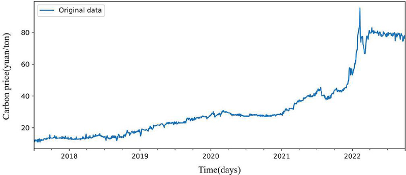
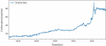
Figure 2 The variation trend of carbon price in GuangDong ETS pilot.
Table 1 Statistical description of carbon price data in Guangdong
| Mean | Max | Min | Std | Skewness | Kurtosis | Jarque-Bera |
| 33.2152 | 95.26 | 11.05 | 20.5780 | 1.2673 | 0.4930 | 344.7642 |
Figure 2 illustrates the trend of changes in the carbon price series for the Guangdong carbon trading pilot utilized in this study. Table 1 provides the statistical description results of the carbon price dataset for the Guangdong carbon trading pilot, calculated using Python 3.9.0. The statistical values reveal that the skewness of the carbon price data is greater than 0, indicating a right-skewed distribution with a longer tail on the right; the kurtosis is less than 3, suggesting a platykurtic distribution; and the Jarque-Bera values are significantly greater than 0, demonstrating that the Guangdong carbon price series does not conform to a normal distribution.
The Augmented Dickey-Fuller (ADF) test results for the Guangdong carbon trading pilot dataset, shown in Table 2, indicate that the ADF test statistics are above their corresponding critical values, with P-values exceeding 0.05, signifying the presence of non-stationary characteristics. The Brock-Dechert-Scheinkman (BDS) test results for the Guangdong carbon trading pilot dataset, obtained through EViews 9.0 and presented in Table 3, exhibit statistical significance at an embedding dimension of 2. The Z-statistics significantly surpass the normal distribution range, with corresponding P-values at 0.0000, thus rejecting the random walk hypothesis. This suggests that the Guangdong carbon price series displays significant nonlinear characteristics.
Table 2 ADF test results
| Threshold | ||||
| 1% | 5% | 10% | T-Statistic | P-value |
| 3.4357 | 2.8639 | 2.5680 | 1.5693 | 0.9978 |
Table 3 BDS test results
| BDS Statistic | Sd | Z-Statistic | P-value |
| 0.2024 | 0.0031 | 66.0256 | 0.0000 |
4.1.2 Data on influencing factors
(1) Structural Factors The price of carbon emission rights is influenced by many factors. In terms of structural impact factors, this paper mainly considers the effects of energy prices, international carbon asset prices, environmental changes, and the financial market.
(2) Energy Prices Industrial production has a significant demand for energy, with the combustion of fossil fuels being the primary source of energy for industrial production. The carbon dioxide produced is the main source of carbon emissions in industrial production. Energy prices are closely related to the production operations of enterprises. Fluctuations in energy prices can lead to changes in energy demand by enterprises, thereby altering their industrial production scale and demand for carbon emission rights, leading to fluctuations in carbon prices.
(3) International Carbon Prices In the globalized economic system, a transnational interdependence and influence network has formed in the carbon market. International carbon prices reflect the global consensus and urgency on carbon emission restrictions. They not only represent the value standard of global carbon reduction efforts but are also an important indicator of international policy trends and market demand changes. As one of the world’s largest carbon emitters, China’s carbon market is influenced by international carbon market trends, especially in carbon trading mechanisms, carbon pricing strategies, and carbon reduction technologies. Fluctuations in international carbon prices can indirectly adjust the supply and demand relationship in China’s carbon market by affecting the cost structure and investment decisions of Chinese enterprises and international trade conditions, thereby affecting carbon prices. Furthermore, compared to more mature carbon markets like the European Union, China’s carbon market is still in its infancy and development stage. Therefore, international carbon prices also serve as a reference and benchmark, guiding China’s strategy adjustments and policy making in global climate change measures. Their changes and fluctuations will to some extent affect China’s carbon prices.
(4) Macroeconomic Shocks Macroeconomic development is driven by the collective action of various industries. On one hand, the macroeconomic level determines the production scale of each industry and the resulting carbon emissions; on the other hand, the macroeconomic situation prompts enterprises to make corresponding production target decisions, thereby affecting the carbon emission demands of enterprises and ultimately influencing carbon prices.
(5) Financial Market The continuous development of the carbon market has increasingly highlighted its financial attributes, and its relationship with traditional financial markets is becoming closer, with a risk spillover effect existing between them. Domestic traditional financial markets mainly affect carbon prices through exchange rates and interest rates. Fluctuations in exchange rates directly affect import and export trade, thereby affecting enterprise production; fluctuations in interest rates directly affect the loan costs and emission reduction costs of enterprises, impacting carbon emissions and causing changes in carbon prices.
(6) Environmental Changes One of the dominant factors affecting carbon trading prices in the climate environment is temperature. In extremely hot or cold environmental conditions, people will increase the frequency of using cooling equipment or increase the demand for thermal supply, leading to an increase in energy demand and CO emissions, thus affecting carbon trading prices. On the other hand, the content of greenhouse gases in the air directly determines the pricing of carbon trading prices. In recent years, air pollution has become increasingly severe, with the massive emission of “three wastes” leading to worsening air quality and serious smog weather. Environmental departments have established the Air Quality Index (AQI) to measure the air quality level. AQI intuitively reflects the content of greenhouse gases in the air, thereby affecting the direction of carbon trading prices.
4.1.3 Non-structural factors
Unstructured data refers to information that lacks a regular structure or is incomplete, without predefined data models. Non-structural influencing factors may conceal significant information, and incorporating this data can lead to a more comprehensive understanding and thus more accurate predictions. Internet search information can reflect people’s psychological expectations and behavioral characteristics in investment decisions in real time. Compared to the Google Index, the Baidu Index provides a higher contribution rate of information for predicting the behavior of domestic residents. Therefore, this paper selects the Baidu Search Index (SI) as the source of non-structural data. The selection of keywords is a prerequisite for obtaining non-structural data using the Baidu Index.
Currently, methods for determining keywords for the Baidu Index include direct selection, range selection, and technical selection. Although the technical selection method yields results with high precision, it has a high computational complexity and requires the support of powerful computing resources to determine keywords. To improve efficiency in keyword selection, this paper initially adopts the direct selection method, using multiple rounds of group discussions and expert reviews to determine the initial keywords. Subsequently, the range selection method is used, applying Baidu’s related word classification and demand graph functions to further select keywords.
This paper selects 13 keywords most likely to reflect residents’ carbon trading behavior, including carbon, low carbon, carbon sink, carbon trading, carbon emission, carbon footprint, carbon neutrality, carbon peak, carbon tariff, low-carbon economy, energy conservation and emission reduction, greenhouse gases, and greenhouse gas emissions, and retrieves the corresponding Baidu Index for these keywords. The final Baidu search index value is the sum of the search volumes for all keywords.
In summary, this paper selects corresponding variables to represent the various types of factors that may influence carbon prices, as detailed in Table 4. Data for all variables in the table are selected for the same time period to match the carbon price series, and linear interpolation is used to fill in missing values. The data on influencing factors all come from the Wind database and are consistent with the Guangdong carbon pilot dataset.
Table 4 Classification of influencing factors and selection of variables
| Type | Variable |
| Energy Price Factors | NYMEX natural gas futures closing price (NG) West Texas Intermediate crude oil futures settlement price (WTI) Brent crude oil futures settlement price (BRE) Coking coal futures closing price (CC) |
| Financial Factors | USD/CNY exchange rate (E/R) EUR/CNY exchange rate (U/R) |
| Economic Factors | China Securities Index 300 closing price (CSI300) |
| International Carbon Emission Prices | European Union Allowance futures price (EUA) |
| Environmental Factors | Daily Air Quality Index (AQI) Highest temperature (HD) Lowest temperature (LD) |
| Non-structural Factors | Baidu Search Index (SI) |
4.2 Evaluation Metrics
To accurately assess the predictive performance of each model, this paper uses three metrics as evaluation criteria: the root mean square error (RMSE), mean absolute error (MAE) and mean absolute percentage error (MAPE). The smaller the RMSE, MAE, and MAPE values of a model, the smaller the error between its predicted values and actual values, demonstrating a better predictive accuracy of the model. Let represent the actual carbon price at time , be the predicted carbon price at time , be the average of actual carbon prices at time , and be the number of prediction samples. The calculation formulas for each metric are as follows:
| (25) | |
| (26) | |
| (27) |
4.3 Parameters and Environment
In this paper, the forecast at a given time point is related to its carbon price over the past 30 days, that is, utilizing the carbon prices from the past 30 days of a specific time point to predict its price. To counteract the randomness inherent in the algorithms, the average outcomes from ten runs of each model are taken as the final prediction results. The VMD layer count is set to 10. For the PSO, the population size is 20, with a total of 100 iterations, and particle velocity ranges between [5, 5]. The experiments were conducted on a computing environment equipped with an R7-5800H CPU, 16.0 GB of RAM, and a Windows 11 64-bit operating system. The setup included TensorFlow 2.5.0 installed, with Python as the programming language, specifically version 3.9.0.
4.4 Forecasting Process
4.4.1 Secondary decomposition
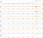
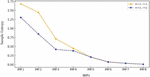
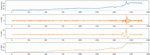
Initially, the CEEMDAN method is employed to decompose the original carbon price series, yielding eight intrinsic mode functions (IMFs), as illustrated in Figure 3. Subsequently, the SE values of all IMFs are calculated, and their complexity is analyzed. Subsequences with similar entropy values are aggregated through component reconstruction to enhance computational efficiency and prevent information loss due to excessive decomposition. Higher SE values indicate greater complexity of the component. As shown in Figure 4, under two parameter combinations, the SE values of IMF1 and IMF2 are both greater than 1, significantly higher than those of other components, while the SE values of IMF6 to IMF8 are all less than 0.1, indicating relatively lower complexity and a clear trend. Therefore, IMF1 and IMF2, IMF3 to IMF5, and IMF6 to IMF8 are aggregated and reconstructed into high-frequency, low-frequency, and trend series, respectively. The aggregation results of each series can be seen in Figure 5.
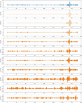
Lastly, the high-frequency series undergoes secondary decomposition using the Variational Mode Decomposition (VMD) algorithm, resulting in ten new intrinsic mode functions, as depicted in Figure 6. The decomposed subsequences exhibit more regularity and predictability compared to the original high-frequency components.
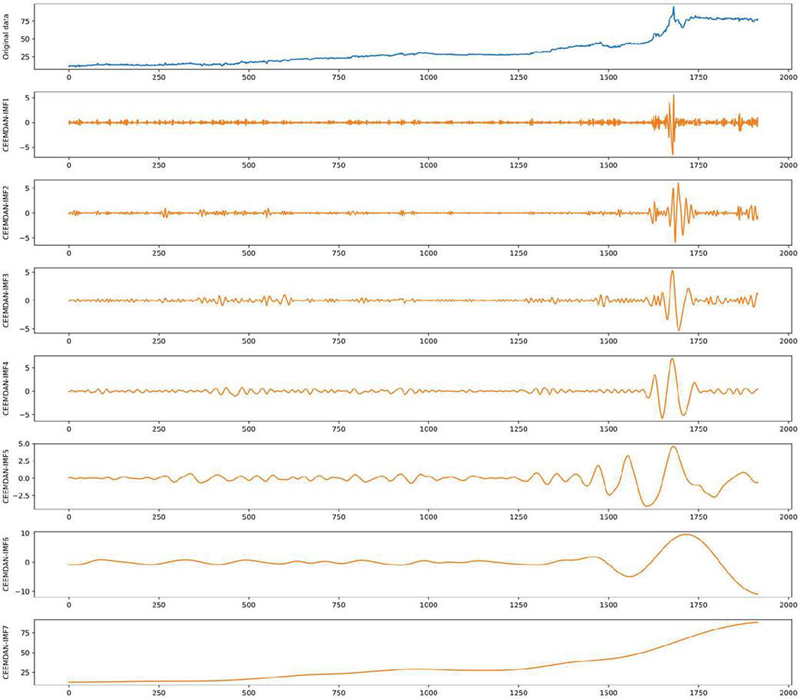
Figure 3 Decomposition results of CEEMDAN.
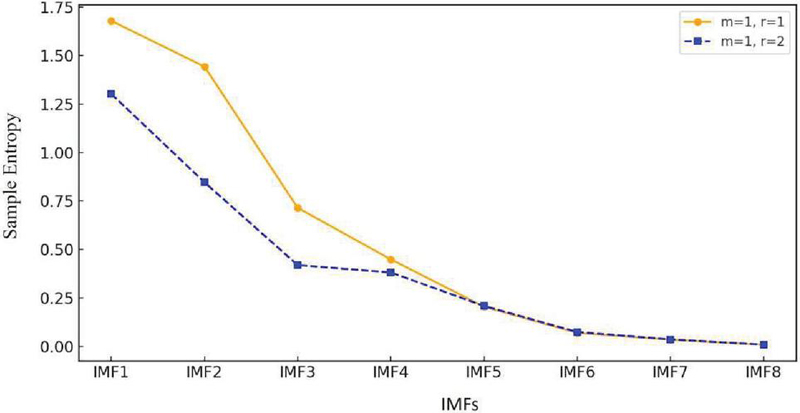
Figure 4 Sample entropy of each IMF with different parameters.
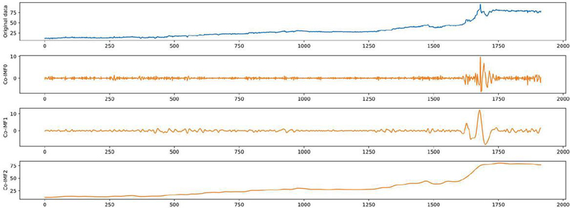
Figure 5 The aggregation results of each component sequence.
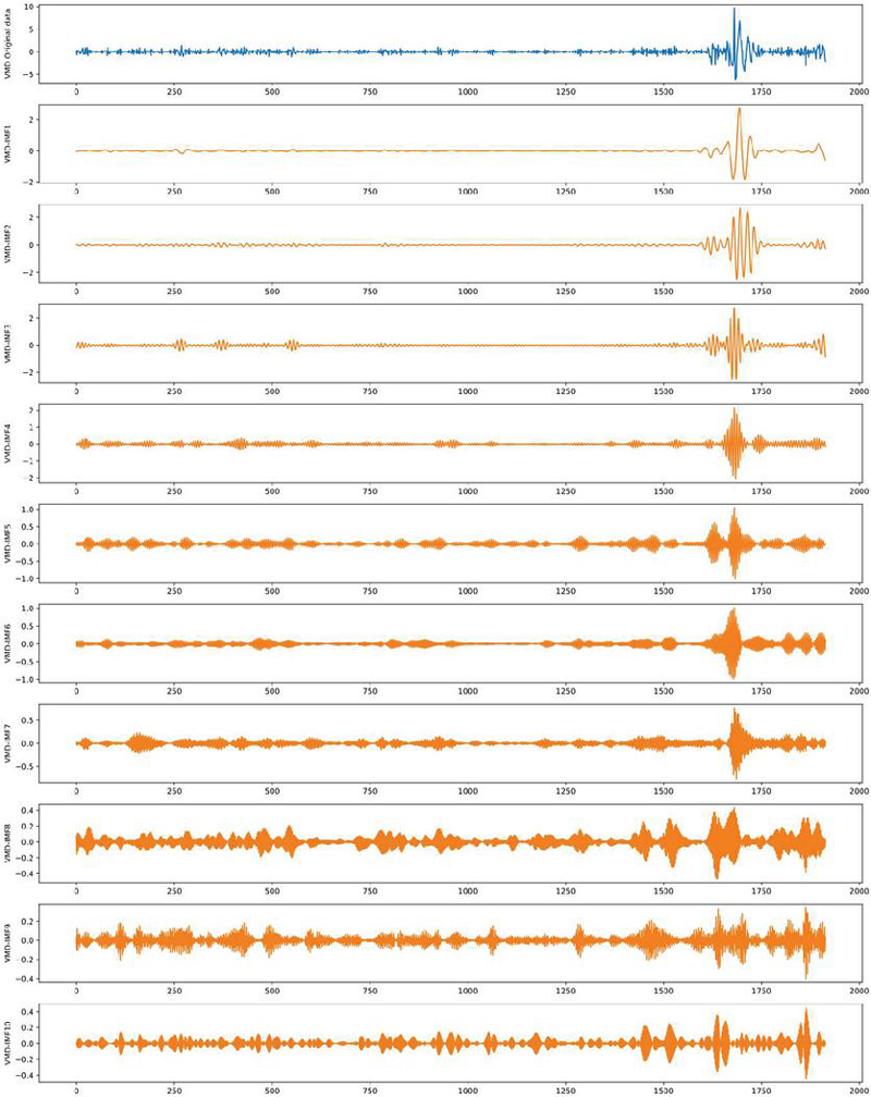
Figure 6 Decomposition result of VMD.
4.4.2 Feature selection
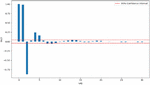
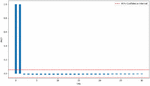
To ensure the accuracy and effectiveness of the model, feature selection methods are employed to determine the input variables of the internal characteristics for the subsequences V-IMFs (obtained after the secondary decomposition of the high-frequency, low-frequency, and trend series. The Partial Autocorrelation Function (PACF) results of the 0 to 30th order for the low-frequency and trend series are calculated. Lags exceeding the 95% confidence interval in the PACF results are selected as input variables for the low-frequency and trend series. As illustrated in Figures 7 and 8, lags that surpass the red dashed line in PACF values are considered key features for the low-frequency and trend series. Table 5 displays the specific results of input variable selection, indicating that the input for the low-frequency series is x, with an input dimension of 2. This presents a difference from the trend series, suggesting that these two series possess distinct characteristics.
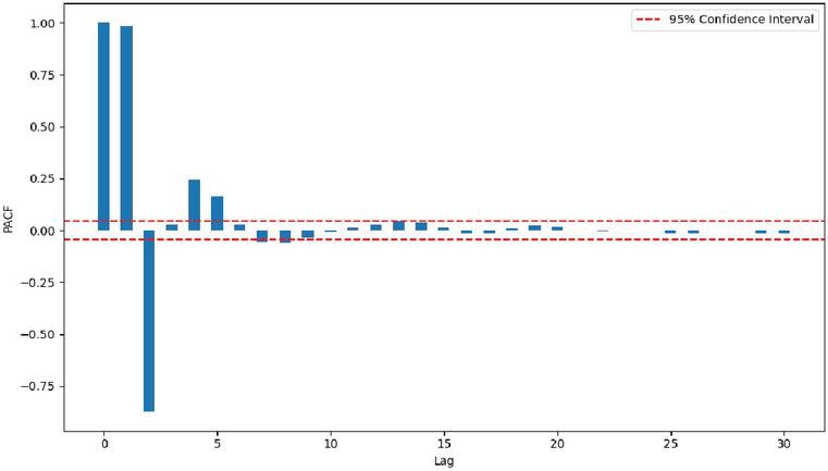
Figure 7 PACF results of low frequency sequences.
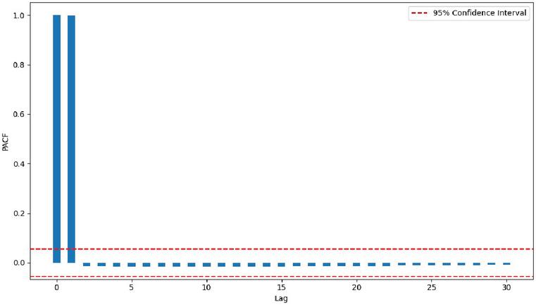
Figure 8 PACF results of trend sequences.
Additionally, the RF algorithm is introduced to calculate the relative importance of the ten sub-sequences of the high-frequency series. Random Forest is an efficient machine learning technique that improves overall prediction accuracy and stability by constructing multiple decision trees and integrating their prediction outcomes. During this process, the algorithm evaluates the contribution of each sub-sequence to the model’s predictive performance, thereby identifying the most important sub-sequences. Based on the calculations (see Table 6 for details), the five most important sub-sequences were selected from these ten, to serve as input variables for the high-frequency series. These five sub-sequences, in descending order of importance, are: V-IMF3, V-IMF10, V-IMF5, V-IMF6, and V-IMF7. This indicates that these five sub-sequences have a decisive impact on predicting the high-frequency part of the Guangdong carbon price series.
Table 5 Low frequency and trend sequence input variables
| Sequence | Input Variable | |||||||
| Low frequency sequence | ||||||||
| Trend sequence | — | — | — | — | — | — | ||
Table 6 RF value of high frequency sequence
| Sequence | RF Value of High Frequency Sequence |
| V-IMF1 | 0.0799 |
| V-IMF2 | 0.0817 |
| V-IMF3 | 0.1980 |
| V-IMF4 | 0.0585 |
| V-IMF5 | 0.1155 |
| V-IMF6 | 0.0967 |
| V-IMF7 | 0.0966 |
| V-IMF8 | 0.0716 |
| V-IMF9 | 0.0779 |
| V-IMF10 | 0.1236 |
Table 7 MIC and Pearson phase relationship values of each influencing factor variable
| Influencing Factor Variable | MIC | Pearson |
| SI | 0.7817 | 0.6376 |
| EUA | 0.8751 | 0.9481 |
| WTI | 0.7224 | 0.7112 |
| BRE | 0.7159 | 0.6755 |
| HS300 | 0.6418 | 0.3728 |
| U/R | 0.6327 | -0.1944 |
| E/R | 0.6327 | -0.8361 |
| NG | 0.7108 | 0.7916 |
| CC | 0.7911 | 0.7911 |
| AQI | 0.1476 | — |
| HD | 0.4866 | — |
| LD | 0.4849 | — |
After completing the feature selection for internal factors, the selection of external factors’ features is conducted. Given the differences in measurement units among the influencing factor variables, the min-max normalization method is first applied to standardize the dimensions of each variable. Subsequently, the selected structured and unstructured influencing factor variables, along with the original carbon price series, undergo MIC analysis. In this analysis, influencing factors with MIC values exceeding 0.5 are selected to ensure their richness in information. Based on this, the Pearson correlation coefficients of the selected influencing factor variables are calculated to identify factors with strong correlation (correlation coefficient greater than 0.5) with the target variable, thereby determining the final external feature input variables. According to the results shown in Table 7, the MIC values and Pearson correlation coefficients for the European Union carbon trading price (EUA) are the highest, underscoring the significant correlation between international carbon prices and carbon price forecasting. In contrast, the Daily Air Quality Index (AQI) presents the lowest MIC values. Additionally, the MIC values for other environment-related influencing factor variables are also below 0.5, indicating that environmental factors have a relatively limited impact on carbon price prediction. The final external feature input variables identified include the EUA, SI, WTI, BRE, NG, and CC. These six influencing factor variables play a decisive role in predicting carbon prices.
4.4.3 Multiscale forecasting
Initially, the high-frequency, low-frequency, and trend series, after feature selection, are forecasted using three predictive models: PSO-BiLSTM, ARIMA, and PSO-XGBoost. During this process, special attention is given to using the trend series and influencing factor variables as joint inputs for the forecast, to fully leverage their correlation. The MIC analysis revealed that the trend series shows a stronger correlation with the influencing factor variables compared to the high-frequency and low-frequency series, possibly because the trend series better reflects long-term market trends and the impact of macroeconomic factors. Hence, the influencing factor variables and the trend series are jointly used as inputs for forecasting, aiming to more accurately capture and learn the key information in the trend series.
Subsequently, the PSO-BiLSTM model integrates the three scales of forecast results obtained in the above process, achieving the final prediction of carbon prices. This integration method combines the unique perspectives and strengths of each series and model, fully capturing the characteristics of carbon price fluctuations and reducing the bias or uncertainty that any single model may introduce. This results in a comprehensive and integrated carbon price forecasting model that provides more robust and accurate predictions. For example, the PSO-BiLSTM model excels in handling non-linear and complex data relationships, the ARIMA model is suitable for linear and stable data sequences, and the XGBoost model excels in effectively integrating and analyzing a large number of influencing factors, capturing subtle changes and deep data relationships that traditional models may overlook. By combining the unique advantages of these models, the multiscale integrated combination forecasting method established in this study not only reflects the immediate dynamics of the market but also considers long-term trends and external influencing factors, offering a comprehensive and in-depth perspective for carbon price forecasting.
Figure 9 shows the final fitted forecast results, clearly demonstrating the excellent performance of the composite forecasting model constructed in this study in predicting carbon prices in the Guangdong carbon market. The figure reveals a high alignment between the model’s predicted values and the actual carbon prices, highlighting the model’s effectiveness in handling complex data and forecasting market dynamics.
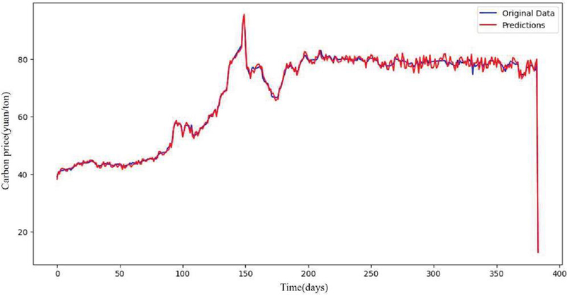
Figure 9 Fitting prediction results of Guangdong carbon pilot.
4.5 Model Evaluation and Comparative Analysis
To validate the effectiveness of the proposed composite forecasting model, nine models were established for comparative analysis. Since some comparison models include many sub-models, all models are named M1–M12 for simplicity. Except for models M5 and M6, all models incorporate unstructured data, predicting with multi-source data inputs such as historical prices, structured influencing factors, and Baidu Index.
The models are detailed as follows: M1: single model XGBoost; M2: single model BiLSTM; M3: XGBoost model optimized with PSO algorithm; M4: BiLSTM model optimized through PSO algorithm; M5: predictions using only historical carbon price data with a multiscale forecasting approach; M6: predictions using a multiscale forecasting approach without unstructured data; M7: based on secondary decomposition and feature selection methods, using multi-source data as input, predicting high-frequency and low-frequency series with PSO-BiLSTM and the trend series and influencing factor data with PSO-XGBoost, and finally integrating all forecast results with PSO-BiLSTM to get the final carbon price forecast; M8: based on secondary decomposition and feature selection methods, using multi-source data as input, predicting all component series and influencing factor data with PSO-BiLSTM model, and integrating all forecast results with PSO-BiLSTM to get the final carbon price forecast; M9: based on the secondary decomposition method, without feature selection for the series, predicting with a multiscale forecasting method; M10: the composite forecasting model proposed in this study The evaluation of the forecasting results of each model is shown in Table 8. Key findings include:
(1) As shown in Figure 9, the forecast results of the proposed composite forecasting model M10 align closely with the actual trends of carbon prices, and its evaluation metrics outperform those of the comparison models, demonstrating excellent forecasting ability. Its RMSE, MAE, and MAPE values are respectively 0.9915, 0.4009, 0.2699, and 0.5183%, indicating good applicability in the Guangdong carbon pilot. Compared to single models M1 and M2, the composite forecasting model significantly improved prediction performance, with optimizations in RMSE, MAE, and MAPE by 84.7%, 85.8%, and 81.4% respectively compared to M1; and 84.2%, 85.8%, and 79.8% compared to M2, proving the effectiveness of the proposed composite strategy in enhancing carbon price prediction accuracy.
Table 8 Error evaluation values for each model
| Methods | RMSE | MAE | MAPE(%) |
| M1 | 2.6159 | 1.9068 | 2.7835 |
| M2 | 2.5307 | 1.9016 | 2.5711 |
| M3 | 2.3749 | 1.7539 | 2.3077 |
| M4 | 2.1531 | 1.7194 | 2.2906 |
| M5 | 1.0261 | 0.9580 | 1.0379 |
| M6 | 0.7011 | 0.5761 | 0.9139 |
| M7 | 0.6749 | 0.5029 | 0.7297 |
| M8 | 0.8515 | 0.7990 | 0.8275 |
| M9 | 0.7490 | 0.6815 | 0.9133 |
| M10 | 0.4009 | 0.2699 | 0.5183 |
(2) By comparing models M1 with M3, and M2 with M4, it is found that the predictive accuracy of both the BiLSTM model (M4) and the XGBoost model (M3) improved with PSO optimization. Specifically, XGBoost (M1) model’s RMSE, MAE, and MAPE decreased by 9.2%, 8.0%, and 17.1% respectively; BiLSTM (M2) saw reductions in RMSE, MAE, and MAPE by 14.9%, 9.6%, and 10.9%. This demonstrates that optimizing the model parameters can fully leverage their predictive capabilities and enhance the precision of carbon price forecasts.
(3) The comparative analysis of models M5, M6, and the proposed composite forecasting model M10 aims to explore the impact of different types of input data on the accuracy of carbon price predictions. The evaluation metrics show that model M6, which includes influencing factor data, significantly outperforms the model M5 that relies solely on historical data. Specifically, the optimization rates of RMSE, MAE, and MAPE for model M6 are 31.7%, 39.9%, and 11.9% respectively. This finding confirms that, compared to relying solely on historical data, incorporating key influencing factors of carbon prices provides richer and more effective feature information for predictions, helping the model to capture anomalies or trend deviations not fully reflected in historical data, thereby improving prediction accuracy. Furthermore, compared to model M6, which does not incorporate unstructured data, the proposed forecasting model M10 demonstrated higher prediction accuracy. The errors in RMSE, MAE, and MAPE for model M10 decreased by 42.8%, 53.2%, and 43.3% respectively, highlighting the important role of unstructured data in enhancing the precision of carbon price predictions. This is because the inclusion of unstructured data captures public attention, enriches the feature set of the prediction model, and provides a more comprehensive perspective for accurate carbon price forecasting.
(4) The multiscale forecasting strategy proposed in this study incorporates three prediction models, specifically utilizing PSO-BiLSTM, PSO-XGBoost, and ARIMA to forecast different series based on the characteristics of their frequency components. Model M7 uses only the PSO-BiLSTM model for all series predictions, while model M8 does not employ ARIMA for low-frequency series forecasting. Compared to the multiscale forecasting model M10, these two models show lower prediction accuracy. Relative to model M7, M10’s RMSE, MAE, and MAPE decreased by 40.6%, 46.3%, and 29.0% respectively; compared to model M8, they decreased by 52.9%, 66.2%, and 37.4%. This demonstrates the effectiveness of the proposed multiscale forecasting strategy in carbon price prediction.
(5) Compared to model M9, which does not feature select for the series, M10 exhibited superior prediction performance, with optimizations in RMSE, MAE, and MAPE of 46.5%, 60.4%, and 43.2% respectively. These results highlight the significant role of the feature selection strategy proposed in this study in enhancing the accuracy of carbon price predictions. The process of feature selection identifies and selects key features with significant impact on the prediction target from a large set of potential explanatory variables, reducing interference from irrelevant features and optimizing the model’s information processing capability. This process not only reduces model complexity and the risk of overfitting but also enhances the model’s ability to capture the intrinsic patterns of the data, thereby improving the precision and reliability of the forecast results.
5 Conclusion and Future Work
Carbon trading is recognized as the most cost-effective method for reducing emissions. Accurate prediction of carbon trading prices can serve as a theoretical reference for the establishment and development of the carbon market. To enhance the accuracy of carbon price forecasting, this study deeply analyzes historical carbon prices and incorporates unstructured data and other external factors affecting carbon prices. This approach captures and understands the complex dynamics affecting carbon price fluctuations more precisely and comprehensively. Additionally, the study employs secondary decomposition and feature selection strategies to minimize data noise and redundant features, optimizing model inputs. Furthermore, a multiscale forecasting strategy is proposed, modeling different frequency components based on decomposition results, enabling the prediction model to capture carbon price patterns across multiple scales and thus improve the model’s feature extraction capability and forecasting accuracy.
In the process of feature selection and analysis, it was found that international carbon prices are highly correlated with the fluctuations in China’s carbon market, while the correlation with environmental factors is lower, despite their perceived impact on carbon prices. Moreover, energy prices also significantly affect carbon price fluctuations. These findings provide valuable insights into understanding carbon price volatility.
This paper establishes nine benchmark models and uses three error evaluation metrics for a comprehensive comparative analysis of model effectiveness. The results show that the feature selection method enhances the model’s ability to capture effective features; parameter optimization helps achieve optimal predictive performance; introducing unstructured and influencing factor data provides a more comprehensive set of information, positively affecting predictive accuracy. Multiscale modeling based on the characteristics of different series further improves predictive performance. The multisource data combination forecasting model, based on feature selection and secondary decomposition, exhibits high predictive accuracy, indicating its suitability as an effective tool for carbon price prediction tasks. In summary, the composite forecasting model proposed in this study provides an effective tool for carbon price forecasting and analysis, offering new directions for developing more efficient and precise forecasting models.
Future research should consider further integrating unstructured data, such as news text, to enrich the model’s insights into key factors like market sentiment, policy changes, and economic events. This integration would provide more comprehensive and timely information on carbon price fluctuations, thereby enhancing the model’s predictive capability and improving the accuracy and reliability of the forecasts.
References
[1] Arouri M E H, Jawadi F, Nguyen D K. Nonlinearities in carbon spot-futures price relationships during Phase II of the EU ETS. Economic Modelling. 2012;29(3):884–892.
[2] Benz E, Trück S. Modeling the price dynamics of CO emission allowances. Energy Economics. 2009;31(1):4–15.
[3] Byun S J, Cho H. Forecasting carbon futures volatility using GARCH models with energy volatilities. Energy Economics. 2013;40(Nov.): 207–221.
[4] Zhang Y, Liu Z, Xu Y. Carbon price volatility: The case of China. PLoS ONE. 2018;13(10):e0205317.
[5] Vapnik V. The nature of statistical learning theory. Springer science & business media. 1999;
[6] Cheng Y, Hu B. Forecasting regional carbon prices in China based on secondary decomposition and a hybrid kernel-based extreme learning machine. Energies. 2022;15(10):3562.
[7] Abdi A, Taghipour S. Forecasting carbon price in the Western Climate Initiative market using Bayesian networks. Carbon Management. 2019;10(3):255–268.
[8] Li H, Huang X, Zhou D, Cao A, Su M, Wang Y, Guo L. Forecasting carbon price in China: a multimodel comparison. International Journal of Environmental Research and Public Health. 2022;19(10):6217.
[9] Zhang F, Wen N. Carbon price forecasting: a novel deep learning approach. Environmental Science and Pollution Research. 2022;29(36): 54782–54795.
[10] Wu Y-X, Wu Q-B, Zhu J-Q. Improved EEMD-based crude oil price forecasting using LSTM networks. Physica A: Statistical Mechanics and its Applications. 2019;516:114–124.
[11] Zhang K, Cao H, Thé J, Yu H. A hybrid model for multi-step coal price forecasting using decomposition technique and deep learning algorithms. Applied Energy. 2022;306:118011.
[12] Deng C, Huang Y, Hasan N, Bao Y. Multi-step-ahead stock price index forecasting using long short-term memory model with multivariate empirical mode decomposition. Information Sciences. 2022;607: 297–321.
[13] Hao H, Yu F, Li Q. Soil temperature prediction using convolutional neural network based on ensemble empirical mode decomposition. Ieee Access. 2020;9:4084–4096.
[14] Zhang Z, Hong W-C. Electric load forecasting by complete ensemble empirical mode decomposition adaptive noise and support vector regression with quantum-based dragonfly algorithm. Nonlinear dynamics. 2019;98:1107–1136.
[15] Huang Y, Yang L, Liu S, Wang G. Multi-step wind speed forecasting based on ensemble empirical mode decomposition, long short term memory network and error correction strategy. Energies. 2019;12(10):1822.
[16] Zhu B, Wang P, Chevallier J, Wei Y. Carbon price analysis using empirical mode decomposition. Computational Economics. 2015;45:195–206.
[17] Sun W, Li Z. An ensemble-driven long short-term memory model based on mode decomposition for carbon price forecasting of all eight carbon trading pilots in China. Energy Science & Engineering. 2020;8(11):4094–4115.
[18] Lu H, Ma X, Huang K, Azimi M. Carbon trading volume and price forecasting in China using multiple machine learning models. Journal of Cleaner Production. 2020;249:119386.
[19] Zhou F, Huang Z, Zhang C. Carbon price forecasting based on CEEMDAN and LSTM. Applied Energy. 2022;311:118601.
[20] Sun W, Huang C. A carbon price prediction model based on secondary decomposition algorithm and optimized back propagation neural network. Journal of Cleaner Production. 2020;243:118671.
[21] Zhou J, Wang Q. Forecasting carbon price with secondary decomposition algorithm and optimized extreme learning machine. Sustainability. 2021;13(15):8413.
[22] Bokelmann B, Lessmann S. Spurious patterns in Google Trends data-An analysis of the effects on tourism demand forecasting in Germany. Tourism management. 2019;75:1–12.
[23] Huang X, Zhang L, Ding Y. The Baidu Index: Uses in predicting tourism flows – A case study of the Forbidden City. Tourism management. 2017;58:301–306.
[24] Almaraashi M. Investigating the impact of feature selection on the prediction of solar radiation in different locations in Saudi Arabia. Applied Soft Computing. 2018;66:250–263.
[25] Dragomiretskiy K, Zosso D. Variational mode decomposition. IEEE transactions on signal processing. 2013;62(3):531–544.
[26] Chen T, Guestrin C. XGBoost: A scalable tree boosting system. Proceedings of the 22nd ACM SIGKDD international conference on knowledge discovery and data mining. 2016;785–794.
Biographies

Shaohui Zou obtained his Ph.D. degree from Xi’an University of Science and Technology. He serves as a doctoral supervisor and is currently the Vice Dean of the School of Management at Xi’an University of Science and Technology. He is also the director of the “Energy Economics and Management Research Center,” a key research base for philosophy and social sciences in Shaanxi higher education institutions. His main research areas are mining and energy economic management, carbon management and environmental policy.

Jing Zhang received the Bachelor’s degree in Management from Xi’an University of Science and Technology and is currently a Master’s candidate at the School of Management of the same university. Her research interests include the prediction and assessment of carbon trading prices.
Strategic Planning for Energy and the Environment, Vol. 43_4, 791–828.
doi: 10.13052/spee1048-5236.4342
© 2024 River Publishers