Optimization and Operation of Microgrid Based on Multi-strategy Collaborative Optimization Salp Swarm Algorithm
Liu Yong1, Pizhen Zhang1,*, Hongping Yang1 and Wang Zhuang2
1Information College of Shenyang Institute of Engineering, Shenyang, 110136, China
2Electrical Engineering College of Shenyang Institute of Engineering, Shenyang, 110136, China
E-mail: zhangpz75@sie.edu.cn
*Corresponding Author
Received 17 May 2025; Accepted 19 July 2025
Abstract
Microgrid systems include various micro power sources that need to meet a large number of constraints. Traditional optimization algorithms often encounter challenges in escaping local optima, making it difficult to achieve optimal solutions. To address such issues, a multi-strategy collaborative optimization algorithm called the multi-strategy collaborative salp swarm algorithm (MSSSA) is proposed, which takes into account both operation and environmental pollution. With the objective function of comprehensive cost, constraints such as power balance, climbing rate, and interaction power extreme value of tie lines are set. Then, the MSSSA is employed to solve the microgrid scheduling model. By comparing the simulation results, the superiority of the MSSSA over other algorithms, as well as the rationality of optimizing microgrid systems, is verified.
Keywords: Microgrid, optimal scheduling, salp swarm algorithm, chaotic mapping, reverse learning strategy.
1 Introduction
At the 75th United Nations General Assembly held on September 22, 2020, China formally committed to two critical environmental targets: peaking carbon emissions before 2030 and realizing carbon neutrality by 2060 [1]. Since then, the “dual carbon” goal has been officially put on the agenda in China. Studies demonstrate that technological innovations can effectively reduce carbon emissions, with North China showing a 23.47% decrease in carbon emission intensity through digital economy development [2], highlighting the importance of advanced energy management systems. The power industry, as an integral part of the national economy, plays a crucial role in people’s daily production and life. The transformation of the traditional power industry is urgently needed to achieve the challenging “dual carbon” goals.” Microgrids, as an emerging clean energy operation mode, have received widespread attention due to their ability to integrate renewable sources and reduce emissions while enhancing grid reliability [3]. Due to its utilization of clean energy sources such as solar and wind energy, it is lower-carbon and more environmentally friendly compared to traditional power systems. It can also directly supply power to users without transmission through the main grid, which is both convenient and efficient. It has great development potential and aligns with our development strategies [4]. However, photovoltaic and wind power generation have the characters of strong randomness and volatility, because they are significantly affected by environmental conditions. Effective operational optimization and power dispatch among diverse energy sources constitute a critical requirement for microgrid management [5].
At present, there have been many studies on optimizing the scheduling and operation of microgrids, and most of them have started from two aspects: optimizing the mathematical model of power sources and improving the intelligent optimization algorithms used [6]. Among them, reference [7] employed the bat algorithm for microgrid operation optimization, targeting minimization of both generation expenses and environmental remediation costs. However, the wind power system was not considered in the modeling of the microgrid, resulting in insufficient environmental protection of the microgrid. Reference [8] incorporated electric vehicle charging/discharging costs while comprehensively accounting for unit operating costs and renewable energy curtailment penalties. The objective function was formulated to minimize the total operational costs throughout the scheduling horizon. The solution employed an enhanced artificial bee colony algorithm, which integrates conventional bee colony optimization with Tenebrio search mechanisms, to solve the proposed model. However, this algorithm is prone to falling into local optima and has low optimization efficiency in the middle stage of solving. Reference [9] established a microgrid optimization configuration model with the minimum energy storage capacity and the lowest operating costs, while accounting for battery-hydrogen hybrid storage system dynamics and operational constraints. The objective functions were to minimize the energy storage capacity and the operating costs, and the corresponding optimization scheme was obtained by applying the improved whale algorithm. However, when establishing constraints, it did not consider the climbing constraints of each micro power source, resulting in inadequate rigor. Reference [10] investigates islanded microgrid systems, proposing a multi-objective genetic algorithm that simultaneously optimizes operational expenditures and environmental impact costs based on their distinctive operational features. Simulation analysis is conducted based on typical daily island microgrid operating data. However, there was no analysis or explanation of the situation during grid connection operation.
As a novel bio-inspired optimization technique, the salp swarm algorithm (SSA) demonstrates superior computational efficiency and structural simplicity compared to conventional intelligent algorithms, particularly in handling high-dimensional optimization problems. However, it also has the common problem of being easily trapped in local optima in intelligent algorithms. The salp swarm algorithm is used to tune current controller parameters and optimize economic dispatch of power loads, but there is little research on using the salp swarm algorithm to optimize economic dispatch of microgrids. To improve this problem, this paper proposes improvement schemes such as chaotic mapping, reverse strategy, and adaptive coefficient. A practical case study of regional microgrid implementation is presented, where the model comprehensively accounts for all micro-generation systems with their physical constraints, with particular attention to environmental cost factors. A microgrid optimization scheduling model is established, and the proposed algorithm is applied for solution. The feasibility and superiority of this algorithm in solving the optimization operation problem of microgrids are demonstrated through comparison.
2 Microgrid Structure and Power Supply Model
2.1 Power Consumption in Data Centers
The overall design of a data center can be classified in 4 categories Tier I-IV each presenting advantages and disadvantages related to power consumption and availability. In most cases availability and safety issues yield to redundant N+1, N+2 or 2N data center designs and this has a serious effect on power consumption. According to Figure 1, a data center has the following main units.
Microgrid architectures are fundamentally categorized into three distinct bus configurations: DC microgrids, AC microgrids, and AC-DC hybrid microgrids [11]. As illustrated in Figure 1, the AC-DC hybrid microgrid integrates both AC and DC buses through a bidirectional converter (AC-DC Exchange), connecting distributed energy resources (WT, PV, MT, FC) and energy storage (Accumulator) to respective AC and DC loads. This hybrid configuration combines the technical advantages of both systems, offering operational flexibility for diverse application scenarios while minimizing energy conversion losses through optimal power routing. The dual-bus architecture significantly enhances system reliability and economic performance compared to single-bus alternatives.
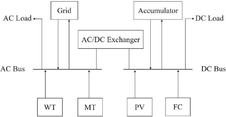
Figure 1 Simple schematic diagram of microgrid system.
Microgrids are designed with flexibility in mind, allowing them to operate in two distinct modes: isolated island mode and grid-connected mode. In isolated island mode, the microgrid functions autonomously, disconnected from the main power grid. This mode is particularly useful during grid outages or when the microgrid needs to operate independently for reasons such as maintenance or optimization of local resources. On the other hand, grid-connected mode enables the microgrid to interact with the larger power grid, allowing for the import and export of power. This mode is beneficial for balancing supply and demand, leveraging economies of scale, and enhancing overall grid stability.
The ability to transition seamlessly between these two modes is facilitated by the operation contact line, which acts as a switch point. This feature allows the microgrid to adapt to varying load requirements and operational conditions. For instance, during periods of high local generation, such as when solar panels are producing excess electricity, the microgrid can export surplus power to the main grid. Conversely, during times of high demand or low local generation, the microgrid can draw power from the main grid to meet its needs. This dual-mode capability enhances the resilience and reliability of the microgrid, making it a valuable asset in modern power systems that are increasingly focused on sustainability and adaptability.
2.2 Mathematical Model of Micro Power Supply
2.2.1 Wind power output model
The operational power output characteristics of wind turbine (WT) generators are governed by a four-regime piecewise function that correlates instantaneous mechanical wind energy capture with electrical power generation, where the output is primarily determined by real-time wind velocity measurements at the turbine’s rotor plane. This relationship can be expressed by Equation (1).
| (1) |
The power output of wind turbines is characterized by several key parameters. represents the variable generation output, while denotes the turbine’s rated capacity under standard conditions. Wind speed plays a crucial role, with v indicating the real-time measurement. The minimum operational speed is , is the optimal rated speed for maximum efficiency, and is the maximum speed before the turbine shuts down automatically. These parameters collectively determine the power output, ensuring the turbine operates efficiently and safely within its designed limits.
2.2.2 Photovoltaic generation model
The electrical power output of photovoltaic (PV) systems can be mathematically modeled as shown in Equation (2), which accounts for both solar irradiance and temperature effects on panel performance.
| (2) |
The photovoltaic power generation output is modeled through several key parameters including the real-time power output , the rated power output under standard test conditions , the reference irradiance at 1000 W/m, and the instantaneous solar irradiance . The model further incorporates temperature-dependent effects through the power temperature coefficient , module operating temperature , and reference temperature at 25C, collectively characterizing the photovoltaic system’s performance under varying environmental conditions.
2.2.3 Fuel cell model
As an electrochemical conversion device [12], fuel cells (FC) transform the chemical energy of natural gas into electricity through redox reactions, bypassing combustion losses. Their operational economics are quantified in Equation (3).
| (3) |
represents the electricity production expenditure, denotes the natural gas price per unit, LHV indicates the fuel’s lower heating value, corresponds to the power output, and signifies the conversion efficiency.
2.2.4 Micro gas turbine model
Micro gas turbine (MT) is a small power generation equipment that generates electricity by burning gas fuel [13], and its cost is expressed as Equation (4).
| (4) |
quantifies electricity production costs, represents fuel price per unit, LHV indicates the energy content of fuel, denotes net power output, and characterizes the system efficiency.
2.2.5 Energy storage device model
Batteries (BAT) are selected as the primary energy storage units in microgrid systems due to their high energy density, high efficiency and good reliability. Its charging and discharging characteristics are crucial for managing power flow and ensuring the stability of microgrids, providing a comprehensive model for predicting the behavior of batteries under various operating conditions. By precisely modeling these characteristics, the system can optimize the use of batteries, thereby maximizing their service life and performance, minimizing the risk of battery degradation, and ensuring that the overall energy management strategy of the microgrid is effective and sustainable. It can be mathematically described by Equation (5).
| (5) |
Among them, characterizes the state of charge at time t, represents the energy storage level at the previous time, and respectively define the charging/discharging power values in time t, and correspond to the energy conversion efficiency of the charging/discharging process, and represents the rated capacity of the energy storage system.
3 Objective Functions and Constraint Conditions
3.1 The Objective Function
In microgrid systems, it is essential to incorporate both operational expenditures and environmental impacts into the overall cost assessment. To optimize the system from an economic standpoint, the objective function formulated for economic dispatch is provided in Equation (6).
| (6) |
In this formulation, denotes the total operational cost of the microgrid, comprising the fuel cost , the operation and maintenance cost , and the grid interaction cost . The parameter serves as a system state indicator, where a value of 1 corresponds to grid-connected operation, and 0 indicates islanded mode.
CF of fuel cost is specifically expressed as Equation (7).
| (7) |
Maintenance cost is specifically expressed as Equation (8).
| (8) |
Let N represent the category of micro power sources, while denotes the management and maintenance coefficient corresponding to the n-th type of micro source. The output power of the n-type source at time t is indicated by .
The cost associated with the interaction between the microgrid and the main power grid is mathematically described in Equation (9).
| (9) |
At time , denotes the unit cost of acquiring electricity from the main grid, while corresponds to the amount of power imported. Conversely, represents the unit price for selling electricity back to the main grid, and refers to the quantity of energy exported during the same interval.
The objective function established considering only environmental cost is Equation (10).
| (10) |
The environmental objective function specifically evaluates the ecological impact costs associated with microgrid operations. In this formulation, enumerates the various categories of emitted pollutants, while corresponds to the remediation expenditure required for the th pollutant type. The total number of distributed generation units is denoted by N. The emission characteristics are quantified through , which represents the mass of pollutant species released per unit energy output from the th generation source. The instantaneous power output from the th micro-generation unit at time interval is given by , characterizes the emission intensity of pollutant associated with each unit of electricity drawn from the main grid, with indicating the real-time power exchange between the microgrid and the central grid system at time .
To simultaneously address both economic and environmental considerations, a multi-objective optimization model is proposed, as formulated in Equation (11).
| (11) |
To promote the dual goals of sustainability and low carbon emissions, the weight coefficients are set as and in this study. The emphasis on environmental costs in the objective function is supported by empirical evidence from China’s carbon market operations. Reference [14] showed that carbon emission costs significantly impact thermal power economics while CCER benefits improve renewable energy profitability, justifying the higher weighting () for environmental factors.
3.2 Constraint Conditions
3.2.1 Power balance constraints
The grid infrastructure plays a pivotal role in this process by enabling bidirectional power flow, connecting renewable sources, storage systems, and end-users [15]. The operational dynamics of the microgrid system necessitate strict adherence to power balance constraints. This fundamental requirement governs the coordinated interaction between distributed generation units, the main utility grid, and end-user demand profiles, as mathematically formalized in Equation (12).
| (12) |
captures the system’s total electrical demand, denotes the instantaneous power production from the ith distributed generator, and governs the bidirectional power exchange with the main utility network. By convention, positive values of correspond to power procurement from the central grid, whereas negative values indicate power export to the grid infrastructure.
3.2.2 Micropower output constraints
To ensure the safe and stable operation of microgrids, the output power of various micro-power sources must be strictly controlled within their rated power range. By preventing the generator sets from exceeding their designed operating parameters, equipment protection can be guaranteed. It can be specifically expressed by Equation (13).
| (13) |
and are the minimum and maximum limits of the power generation capacity of each microsource under different operating conditions.
3.2.3 Contact line interaction power constraints
The power exchange interface with the main grid requires rigorous operational constraints to maintain interconnection stability, with Equation (14) mathematically defining the permissible power transfer limits.
| (14) |
The values and correspond to the maximum and minimum allowable limits of the interactive power, respectively, defining the operational range within which the power exchange must be maintained.
3.2.4 Constraints on charging and discharging batteries
To prevent the occurrence of overcharging and deep discharging, battery energy storage systems need to pay special attention to charge state management. Equation (15) establishes a safe operating boundary for charge retention.
| (15) |
The operational envelope is bounded by (maximum state-of-charge) and (minimum state-of-charge), which are typically set based on battery chemistry and aging considerations.
3.2.5 Climbing rate constraint
For the controllable micro power supply, the constraint of climbing rate should also be satisfied, which is specifically expressed as Equation (16).
| (16) |
Ramp rate limitations, quantified by and , restrict the maximum permissible power variation between consecutive dispatch intervals for each micro-source. These constraints prevent mechanical stress on generation equipment while maintaining power quality standards.
4 Salp Swarm Algorithm and Its Improvement
4.1 Salp Swarm Algorithm
The salp swarm algorithm (SSA) represents a metaheuristic optimization technique that mathematically models the distinctive foraging patterns observed in marine salp colonies [16]. It has the advantages of simple structure and fast convergence. Salps are transparent marine creatures. When moving and hunting, salps form chains to move quickly. According to their position, the salp swarm is divided into two parts: the first half is called the leader, responsible for searching for food, and the second half is called the follower, which follows the leader toward the food source. Suppose that there are N salps foraging in the space of dimension D. Within the SSA framework, each candidate solution is represented as a D-dimensional position vector , , where the population is divided into leaders (first N/2 individuals) and followers. The leaders’ positional update mechanism follows the mathematical formulation presented in Equation (17).
| (17) |
The spatial coordinate denotes the position of salp i along dimension j, while represents the target food source position in the same dimension. The search space boundaries are defined by and , which respectively specify the upper and lower exploration limits in each dimension. Stochastic exploration is controlled through uniformly distributed random variables and within the interval (0,1), while the adaptive convergence coefficient dynamically balances the exploration-exploitation tradeoff throughout the optimization process, and the expression is shown in Equation (18).
| (18) |
This coefficient follows an exponential decay pattern governed by the current iteration index t, maximum iteration count iter, and a decay rate constant k typically set to 2.
The follower update formula is shown in Equation (19).
| (19) |
4.2 Improved Salp Swarm Algorithm
The Salp Swarm Algorithm exhibits inherent limitations common to metaheuristic optimization techniques, including premature convergence to local optima and diminished convergence rates during later iterations. This is especially significant in the case of multi-population and high dimensional conditions. To address these challenges, this study incorporates three key enhancements: chaotic population initialization, opposition-based learning, and an adaptive leadership ratio mechanism. The proposed Multi-Strategy Synergistic Salp Swarm Algorithm (MSSSA) demonstrates superior performance in escaping local optima while significantly enhancing algorithmic robustness.
4.2.1 Chaotic initialization
Conventional random initialization methods often fail to guarantee uniform population distribution, critically impacting optimization performance since solution quality strongly correlates with initial population dispersion characteristics. The chaotic sequence generated by chaotic mapping has strong ergodic property, which can make the initial population position more uniform. The commonly used chaotic sequences include Logistic mapping, Singer mapping and Tent mapping. In this paper, Tent mapping with simple model and good ergodic performance was used to initialize the population [17]. Tent mapping expression is shown in Equation (20).
| (20) |
Beta is the random number between (0,1), usually 0.5. It is explained here that in order to ensure the uniformity of random numbers obtained in each step of the algorithm, the algorithm adopts Tent mapping.
4.2.2 Reverse learning strategy
Adopting the reverse learning strategy can significantly improve the quality and diversity of the population and is an effective method [18]. The basic realization step is to generate the reverse population corresponding to the initial population in the center of the lower limit boundary as the symmetry axis. Following opposition-based generation, the selection operator retains the top N fittest individuals to form the subsequent population, as mathematically formulated in Equation (21).
| (21) |
4.2.3 Adaptive scale change
The standard algorithm maintains a fixed 1:1 leader-follower ratio throughout iterations, which contributes to early-stage stagnation and late-stage precision loss. The introduced adaptive coefficient [19] dynamically adjusts this ratio during optimization, effectively mitigating these limitations through progressive leader-follower rebalancing. The expression of adaptive proportionality coefficient is shown in Equation (22).
| (22) |
is the control coefficient (0.75) and is the disturbance coefficient (0.2).
4.3 Improved Salp Swarm Algorithm Flow
The algorithm flow chart of MSSSA is shown in Figure 2. Initially, the algorithm generates a reverse population, which is subsequently merged with the initial population.
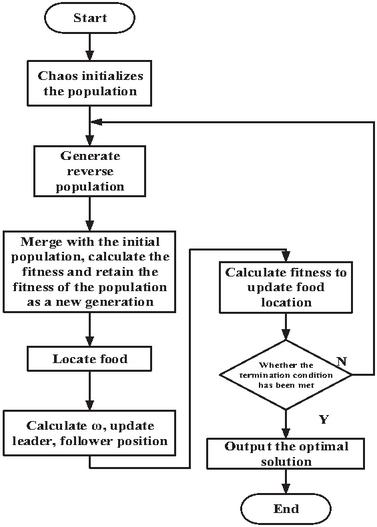
Figure 2 Algorithm flow chart of MSSSA.
This amalgamation is followed by a fitness evaluation to ascertain the quality of solutions, thereby retaining the fittest individuals as a new generation. The algorithm then proceeds to calculate the fitness to update the food location, which serves as a metaphorical representation of the optimal solution in the search space. Subsequently, the food is located, and the parameter (omega) is computed to update the leader and follower positions, guiding the swarm towards more promising regions of the solution space. This iterative process continues until the termination condition is satisfied, at which point the algorithm outputs the optimal solution. The MSSA’s structured approach ensures a balance between exploration and exploitation, enhancing its efficacy in global optimization problems.
5 Example Simulation
5.1 Parameter Settings
The computational experiments were configured with a population size of 100 individuals and a maximum iteration count of 500 generations. The technical specifications for distributed energy resources, including their operational parameters and constraints, are detailed in Table 1. Environmental performance characteristics, particularly emission factors for various pollutants, are presented in Table 2, while the time-of-use electricity pricing scheme governing grid interactions is specified in Table 3.
Table 1 Distributed power supply parameters
| Power | Rated | Fuel | Operation and Maintenance | Climbing |
| Type | Power (kW) | Cost (Yuan/kW) | Cost (Yuan/kW) | Rate (kW/h) |
| WT | 50 | / | 0.314 | / |
| PV | 30 | / | 0.014 | / |
| MT | 70 | 0.358 | 0.038 | 100 |
| FC | 60 | 0.199 | 0.092 | 80 |
| BAT | 40 | / | 0.0017 | / |
Table 2 Pollutant emission coefficient and treatment cost
| MT Emission | FC Emission | Grid Emission | Processing | |
| Coefficient | Coefficient | Coefficient | Cost | |
| Pollutant | (g/kWh) | (g/kWh) | (g/kWh) | (Yuan/kg) |
| CO | 0.053 | 0 | 0.088 | 11.84 |
| CO | 732 | 496 | 894 | 0.25 |
| SO | 0.0041 | 0.004 | 1.86 | 15.037 |
| NO | 0.32 | 0.022 | 1.67 | 65.249 |
Table 3 Timeshare purchase and sale price of micro grid
| Electricity Purchase | Electricity Sale | |
| Time Period | Price (Yuan/kWh) | Price (Yuan/kWh) |
| Valley time (23:007:00) | 0.52 | 0.32 |
| Peace time (8:009:00; 15:0019:00) | 0.87 | 0.63 |
| Peak time (10:0014:00; 20:0022:00) | 1.14 | 0.90 |
Figure 3 illustrates the normalized daily profiles for both electrical load demand and renewable generation outputs, capturing the characteristic diurnal patterns of wind power production and photovoltaic generation specific to this geographical region. These profiles reflect the typical variability and complementarity between these intermittent renewable sources.
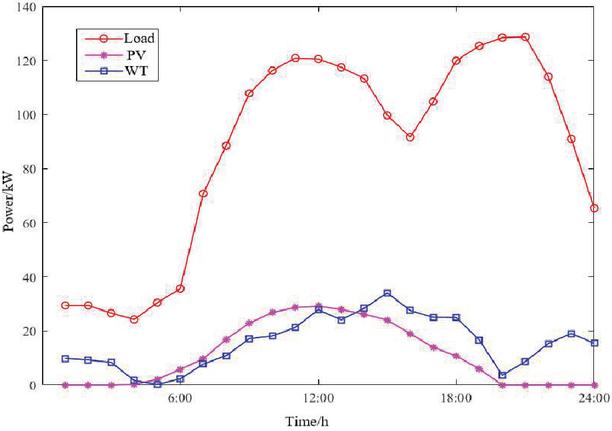
Figure 3 Load, WT and PV output curves.
5.2 Simulation Results and Analysis
A comprehensive comparative analysis was conducted to evaluate the proposed MSSSA against three established optimization techniques: the canonical Salp Swarm Algorithm (SSA), Particle Swarm Optimization (PSO), and Genetic Algorithm (GA). Each algorithm was implemented in MATLAB to solve the microgrid operational optimization problem, with 50 independent runs performed to ensure statistical significance of the results. The convergence characteristics and solution quality metrics from these comparative trials are visualized in Figure 4.
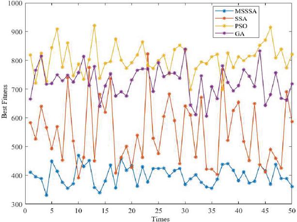
Figure 4 Optimal fitness distribution of each algorithm after 50 runs.
As shown in the figure, although the traditional PSO and GA algorithms have relatively uniform distributions and stable curve fluctuations, they cannot obtain good fitness values. Although SSA can obtain better fitness values, it has the worst stability and the largest curve fluctuations. MSSSA can not only obtain the best fitness value, namely the scheduling scheme with the minimum economic cost, but also the most uniform distribution of the optimal fitness value and the least fluctuation of the curve, so it is the best optimization algorithm among the four algorithms. Quantitative performance metrics, including central tendency measures (mean, median), dispersion statistics (standard deviation), and extreme values (optimal and worst-case solutions) across all algorithm trials, are systematically compared in Table 4. This statistical analysis provides rigorous evidence of algorithmic performance differences.
Table 4 Comparison of algorithm solution results
| Algorithm | Mean Value | Sd | Median | Best Value | Worst Value |
| GA | 725.2844 | 53.0066 | 523.8306 | 606.5399 | 838.5192 |
| PSO | 805.3134 | 49.6285 | 805.7631 | 697.7264 | 921.5261 |
| SSA | 549.3611 | 112.5163 | 523.8306 | 391.6459 | 822.3750 |
| MSSSA | 399.4790 | 33.2688 | 395.9495 | 330.6413 | 469.2941 |
The optimized dispatch schedules for distributed energy resources are presented in Figure 5, depicting the temporal allocation of generation across various micro-sources. Complementary to this, Figure 6 quantifies the bidirectional power exchange dynamics between the microgrid and main utility grid, highlighting periods of net import versus export conditions.
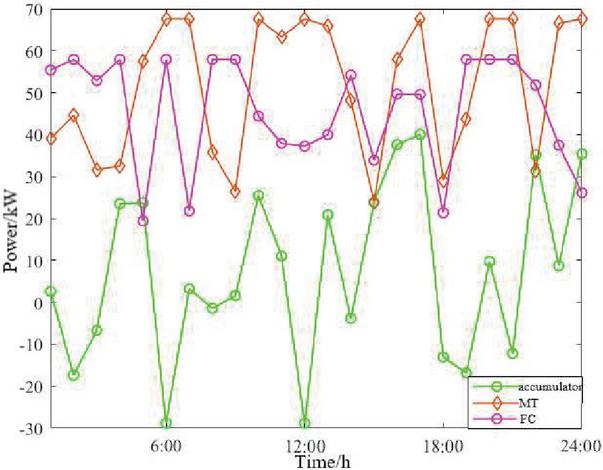
Figure 5 Treatment of each micro power supply.
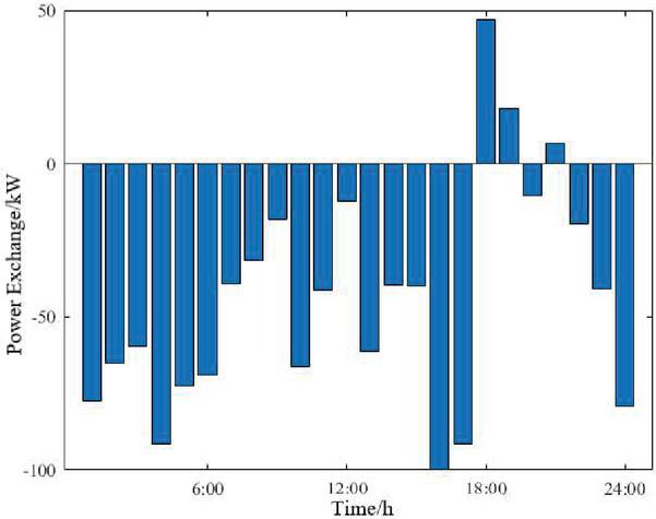
Figure 6 Power exchange between microgrid and large grid.
Analysis of the operational patterns in Figures 5 and 6 clearly demonstrates the microgrid’s adaptive energy management under different demand scenarios. During low consumption periods, microturbines and fuel cells work in tandem to collectively satisfy the load requirements while generating surplus power for profitable grid export, thereby significantly enhancing system revenue. The evening peak between 18:00 and 19:00 presents substantial operational challenges as solar generation diminishes to negligible levels and wind resources decline, creating conditions that necessitate supplemental power procurement from the main grid to maintain a reliable supply. Throughout these varying operational states, the integrated battery storage system provides essential regulation capabilities, dynamically balancing generation and consumption to achieve both operational reliability and economic efficiency, ensuring the microgrid operates smoothly and cost-effectively.
6 Conclusion
This study presents the architecture and composition of a typical microgrid, formulates mathematical models for each micro-power source, and constructs the objective function along with the associated constraints for optimization. Subsequently, the fundamental Salp Swarm Algorithm is introduced and enhanced. The improved algorithm is applied to address the optimal scheduling model of microgrid simulations. Through chaotic population initialization and opposition-based learning mechanisms, the algorithm significantly improves the quality of initial solutions and enhances population diversity, effectively preventing premature convergence issues that plague traditional algorithms in “generation-grid-load-storage” multi-variable coupling scenarios.
The enhanced Salp Swarm Algorithm developed in this research effectively addresses the optimal operation of microgrids within the context of the new power system, particularly under the “dual carbon” goals. It is well-suited for microgrid systems that integrate “source, network, load, and storage” collaboration, thereby providing a robust foundation for further exploration of advanced optimization techniques in microgrid operations. In future research, the optimal operation and stability of microgrids after the addition of electric vehicles will be analyzed to better align with energy-saving requirements and promote the realization of low-carbon living.
Acknowledgements
This paper is supported by the Natural Science Foundation of the Liaoning Provincial Science and Technology Joint Program under Grant No. 2024-MSLH-329.
Conflicts of Interest
The authors declare that they have no conflicts of interest to report regarding the present study.
References
[1] Shu Yin-biao, Zhang Li-ying, Zhang Yun-zhou, et al. (2021). Carbon peak and carbon neutrality path for China’s power industry. Strategic Study of CAE, 23(6): 1–14.
[2] Dongfang Dai. (2024). Influence of Digital Economy on Ecological Carbon Environment in North China Under Spatiotemporal Synergistic Evolution. Strategic Planning for Energy and the Environment, 43(04), 961–978.
[3] Moslem Uddin, Huadong Mo, Daoyi Dong, Sondoss Elsawah, Jianguo Zhu, Josep M. Guerrero. (2023). Microgrids: A review, outstanding issues and future trends, Energy Strategy Reviews, (49): 101–127.
[4] Meng Ming, Chen Shi-chao, Zhao Shu-jun, Li Zhen-wei, Lu Yu-zhou. (2017). Overview on Research of Renewable Energy Microgrid. Modern Electric Power, 34(01):1-7.
[5] Li Bowen, Le Bin, Liu Yu-fen, (2016). Summary of research on economic dispatching of microgrid. Technology Innovation and Application, (23): 216.
[6] Nie Han, Yang Wen-rong, Ma Xiao-yan, et al. (2019). Optimal scheduling of islanded microgrid based on improved bird swarm optimization algorithm. Journal of Yanshan University, 43(3): 228–237.
[7] Zhang Yi-shu, Li Yi-lun, Song Guang, Niu Jun. (2022) Research on Microgrid Optimization Based on Bat Algorithm. Northeast Electric Power Technology, 43(04): 4–10.
[8] Wang Shao-lin, Wang Gang, Wang Xiao-lei, Wang Hai-long, Yang Jin-cheng, Huang Zhao-yang, Liu Hong-peng. (2022). Optimal scheduling of electric vehicle microgrid based on improved bee colony algorithm. Electrotechnical Application, 41(04): 63–70+13–14.
[9] Hao Xiao-hong, Wang Rui, Pei Ting-ting, Huang Wei. (2022). Research on Mircogrid System Capacity Optimization Based on Improved Whale Algorithm. Automation & Instrumentation, 37(03): 11–16.
[10] Li Jia-xin. (2022). Research on Optimal Scheduling of multi-objective microgrid based on Genetic Algorithm. China Plant Engineering, (03): 137–139.
[11] Gao Yu, Huang Sen, Chen Liu-xin, Huang Jun-hu. (2020). Economic Optimization Scheduling of Grid-connected Alternating Microgrid Based on Improved Gray Wolf Algorithm. Science Technology and Engineering, 20(28): 11605–11611.
[12] Huang Nian-zhi. (2018). Modeling, Analysis and Optimization of Fuel Cell-based Combined Heat and Power System (Ph.D. Thesis). Shandong University.
[13] Liu Jun, Mu Shi-xia, Li Yan-song. (2010). Overall Modeling and Simulation of Microturbine Generation Systems in Microgrids. Automation of Electric Power Systems, 34(07): 85–89.
[14] Jian Zhang, Qian Sun, Xiaohe Liang, Jian Chen, et al. (2023). LCOE Calculation Method Based on Carbon Cost Transmission in an “Electricity-Carbon” Market Environment. Strategic Planning for Energy and the Environment, 42(04), 647–672.
[15] Tian, X., Zhao, L., Zhao, E., Qiu, X., Li, S., and Li, K. (2024). Enhancing Resource Allocation for Multi-Energy Storage Systems: A Comprehensive Approach Considering Supply and Demand Flexibility and Integration of New Energy. Strategic Planning for Energy and the Environment, 43(03), 665–684.
[16] Mirjalili S, Gandomi A H, Mirjalili S Z. (2017). Salp Swarm Algorithm: A Bio-inspired Optimizer for Engineering Design Problems. Advances in Engineering Software (S1873-5339), 114(6): 163–191.
[17] Long Wen, Cai Shao-hong, Jiao Jianjun, et al. (2019). An improved grey wolf optimization algorithm. Acta Electronica Sinica, 47(1): 169–175.
[18] Zhou Rong, Li Jun, Wang Hao. (2020). Reverse learning particle swarm optimization based on grey wolf optimization. Computer Engineering and Applications, 56(7): 48–56.
[19] Liu Jing-sen, Yuan Meng-meng, Li Yu. (2021). Solving Engineering Optimization Design Problems Based on Improved Salp Swarm Algorithm. Journal of System Simulation, 33(04): 854–866.
Biographies

Liu Yong received his B.S. degree form Tohoku University in 2004, his M.S. degree from DongBei University Of Finance & Economics in 2006. He is currently a lecturer in Shenyang Institute of Engineering. His research interests include communication network and Big Data Analysis.

Pizhen Zhang received his B.S. degree from LiaoNing Normal University in 1998, his M.S. degree from Northeastern University in 2006. He is currently a associate professor in Shenyang Institute of Engineering. His research interests include cyberspace security, machine learning, big data analysis and processing.

Hongping Yang received the Bachelor’s Degree from Northeast Forestry University (China). March 2005, awarded the Master of Science in Computer Science from California State University (United States). Currently serves as a Professor at Shenyang Institute of Engineering, primarily engaged in research and teaching in network application development and cloud computing.

Wang Zhuang received the Bachelor of Engineering in Energy and Power Engineering from Shenyang Institute of Engineering. In April 2024, awarded the Master of Engineering in Electrical Engineering from Shenyang Institute of Engineering. Currently employ by State Grid Liaoning Panxian County Electric Power Supply Company.
Strategic Planning for Energy and the Environment, Vol. 44_4, 859–880.
doi: 10.13052/spee1048-5236.44410
© 2025 River Publishers