Optimal Placement of Distributed Generators and Capacitors for Power Loss Reduction Using Crested Porcupine Algorithm
Shilpa Phatak1,*, L. S. Titare2 and A. K. Sharma1
1Electrical Engineering Department Jabalpur Engineering College Jabalpur (MP), India
2Electrical Engineering Department Ujjain Engineering College Ujjain (MP), India
E-mail: shilpaacademics2@gmail.com
*Corresponding Author
Received 30 September 2025; Accepted 12 June 2026
Abstract
In recent years, as the need for energy rises, the application of dispersed generation and shunt capacitors has become a more common solution to meet the growing demand of energy. The article presents a novel approach to optimise radial distribution networks, called the Crested Porcupine optimisation algorithm (CPOA), inspired by the behaviour of the Crested Porcupine. The proposed method is tested on the IEEE system, which has 33, 69 and 85 buses. The purpose of this work is to lower the cost and power loss while improving the voltage profile and voltage stability index (VSI) using the Capacitor Banks (CB) and Distributed Generator (DG) units at the correct location and of appropriate size. Inclusion of load models is also taken into consideration.
Keywords: Voltage profile, power loss, distributed generation, capacitor bank and voltage stability index.
Nomenclature and Abbreviations
| CPOA | Crested porcupine optimization algorithm | IA | Improved Analytical |
| VSI | Voltage stability index | SSO | Shark Smell Optimization |
| CB | Capacitor bank | AT | Analytical Technique |
| DG | Distributed generation | In | Branch current |
| RDN | Radial distribution network | Rn | Branch resistance |
| MO | Multi objective | Nb | Number of buses |
| MFO-SCA | Moth flame optimization and Sine Cosine algorithm | RPL | Reduction in power loss |
| ECOA | Enhanced Coyote optimization algorithm | TVDbase | Total base voltage deviation |
| GA | Genetic algorithm | RPLbase | Total base reduction in power loss |
| PSO | Particle swarm optimization | Minimum active power from DG | |
| IMDE | Intersect mutation differential evolution | Maximum active power from DG | |
| RPL | Reduction in power loss | Minimum reactive power from DG | |
| VSI | Voltage stability index | Maximum reactive power from DG | |
| TVD | Total Voltage deviation |
1 Introduction
On a global scale, insufficiency of power is a well-known issue. This problem is because of the enormous demand for electrical energy. This high demand cannot be met by a centralised power supply. To overcome this issue, distribution networks play an important role. It results in lower voltages and high-power loss. Generally, distribution networks are connected with many kinds of loads, such as commercial, residential, and industrial. The above-mentioned loads are dependent on voltage. After changing the load profile on the demand side, voltage collapse occurs, resulting in an imbalance of power and voltage profile. To suffice all up to a certain extent, integration of dispersed generation or distributed generation into the distribution network is quite popular [1]. By properly incorporating the DG units into the distribution system, overall efficacy can be improved. Likewise, the radial distribution network can be made more efficient by locating CBs and DGs simultaneously using a multi-objective optimization strategy [2].
Many previous literatures are discussed here in brief. Whale optimization and polar bear optimization are described in [3] and [4], respectively, for different bus systems to allocate the capacitors. Using the 24-bus system and the spotted hyena optimizer algorithm, different loading situations are also taken into account in [5]. To achieve the minimum real power loss, an analytical expression and exact loss calculation are given in [6] for the individual allocation of dispersed generators in RDN. for minimization of losses and improvement in voltage profile on IEEE 33,69 and 118 bus systems, simulated annealing and comprehensive teaching-learning based optimization algorithms, respectively, are suggested in [7] and [8]. For the purpose of assigning appropriate sized DG on the 86 bus and 69 bus system, [9] demonstrates multi-objective (MO) optimization employing adaptive particle swarm optimization and a modified gravitational search technique. [10] integrates DG and CBs at the same time to reduce power loss in IEEE 69 and 33 bus distribution systems by implementing a hybrid technique called MFO-SCA (Moth flame optimisation algorithm and sine cosine algorithm). In [11] ECOA is implemented on different distribution systems containing 33, 69, and 85 buses for solving the MO problem. Objectives are to reduce loss and cost and to improve the stability of voltage. [12] and [13] both allocate DG and CB simultaneously using soft-computing techniques such as GA, PSO and cuckoo search optimization, respectively, to find the target. [22] presents an African vultures optimization technique to optimally allocate DG and capacitor banks on 85 and 118 bus systems for minimizing total system cost, and active and reactive line loss. [23] introduces a novel optimization method known as IMDE designed to optimally position and size DGs and CB inside the distribution network. [29] described the modified firefly algorithm on the 85-bus system to improve efficiency and voltage profile. [30] presents Cheetah optimisation on 33 and 69 bus standard distribution systems to achieve the objectives of better power loss and voltage stability.
In the presented approach, the CPOA is implemented to optimize the size and location of type-I DG, type-III DG, CBs, and simultaneous placement of the type-I DG along with CB in different radial networks of distribution system.
2 Problem Formulation
2.1 Power Flow
Radial distribution system has some unique features such as high value of resistance to reactance ratio, unbalanced load, and radial layout. The Forward – backward sweep approach is employed due to the slow convergence of the traditional load flow method. To assess the power from the receiving to the sending end is called forward sweep, while reverse assessment of voltage is under forward sweep.
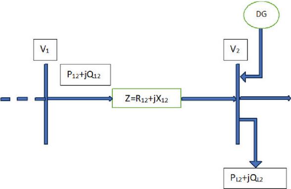
Figure 1 Radial distribution system.
Figure 1 shows radial distribution system with two buses namely bus 1 and bus 2. Active and reactive power flow between bus 1 and 2 denoted by and via branch and bus voltage, can be calculated using Equations (1) to (2), as below
| (1) | ||
| (2) |
Here,
and are real and reactive power of bus 1 and bus 2.
and are voltage of bus numbers 1 and 2, respectively
and are real and reactive power of load connected in second bus
and are the resistance and reactance of the branch connected between bus 1 and 2
| (3) |
Real power with installation of type 1 DG only, type 3 DG only, type 1 and CB simultaneously, can be shown as Equation (3)
| (4) |
Equation (4) shows reactive power flow after inserting only the capacitor bank and the simultaneous insertion of type 1 and capacitors.
After the DG installation of type 3
| (5) |
Reactive power flow can be found by Equation (5) when only type 3 DG is inserted.
Here, and represents real and reactive power injection from DG, and denotes reactive power injection from CB.
Proper installation of DG can effectively support the system performance improvement, such as voltage profile, stability, and power quality [33].
2.2 Objective Function
Now, the objective function can be defined as Equation (6) given below,
| (6) |
here,
and the values of a 0, b 20 & are c 0.25.
Where,
Here, RPL is the reduction in power loss, and VSI is the voltage stability index. TVD is the total voltage deviation, equivalent to the summation of the difference between Vref and the final voltage of all the buses.
2.3 Constraints
There are several limitations related to the goal that can be grouped into two types: Equality and inequality constraints, shown in Table 1.
Table 1 Constraints under the study
| Constraints | Name | Relation |
| Equality | Power balance | & |
| Inequality | Bus voltage & Thermal limit | and |
| DG capacity limit | & | |
| Capacitor bank capacity |
3 Crested Porcupine Optimization (CPO)
Crested porcupine optimization (CPO) is an innovative meta-heuristic technique to solve the optimization problem involving large-scale data sets, evolved by Mohamed Abdel-basset et al. [27]. Crested porcupines shown in Figure 2 are the third largest rodent, following the capybara and the beaver. CPs are giant, slow, and spherical in shape. The majority of CPs have bristles that are either black or dark brown and occasionally appear with white marks. Their most distinctive feature is the broad quills, which may grow up to 14 inches long and run along the back half of their body. The primary characteristic of CPO is the defense strategy of other animals, such as tigers, leopards, and lions. CPs are the most effective defenders. They are regarded as accomplished defenders due to their unique physical traits. As CPs feel threatened, it adapt their defensive tactics through four displays that show aggression.
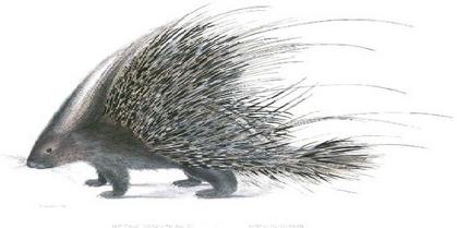
Figure 2 Crested porcupine.
It is based on numerous protective actions of the CP, namely sight, sound, odour, and physical attack, ranging from minimal hostile to highly aggressive. The first two methods (i.e. sight and sound) show exploring behaviour, whereas the third and fourth ones (i.e. odour and physical attack) are considered exploitative.
(i) Vision: It is the very first line of defense. After detecting danger, it defends itself by raising sharp and pointed spines and by elevating its quills to look bigger than they actually.
(ii) Voice: CPs use a wide range of vocalization tactics to notify predators of their impending arrival. On feeling frightened or hostile, CP creates sounds of whining, grunting, coughing, and snoring, and these become louder. They click their teeth, jump erratically, stamp their feet, and make a loud hissing sound with tail quills to survive and protect themselves.
(iii) Smell: When visual and audio stimuli don’t work to repel a predator, this tactic is used. A foul chemical odour is released by CP’s lower back gland. This strategy is often a successful one for fending off dangers.
(iv) Attack: The distinct characteristic of CP is having powerful quill armour, by using these sturdy quills, CP protects itself against potential danger. When approached by a predator, the CP forms a crest and erects its quills to look larger.
CPO has some benefits such as being less sensitive to parameters, consistent, good balance between exploration and exploitation and global search ability. Also, it has some disadvantages like faces problems while dealing with high dimension problem, and it has fast convergence with untuned parameters. Point-wise elaboration of the benefits of CPOA over the standard metaheuristics given below:
(i) Maintain balance between exploration and exploitation: CPOA has two local exploitation operators along with two global exploration operators. This makes CPOA superior to the other algorithms (such as GSA, PSO and SSA) suffers from local optima trapping.
(ii) Enhanced local optima trapping: Due to the incorporation of a cyclic population reduction strategy, some individuals are removed and re-enter for maintenance of the diversity of the population. Due to this mechanism, CPOA does not face the problem of local minima, unlike other algorithms (PSO, GSA).
(iii) Less sensitive to parameters: It shows robust performance in different parameter settings. Due to this, CPOA shows lower risk for poor performance in case of improper selection of parameters, unlike other algorithms.
(iv) Higher speed and convergence: CPOA can achieve a solution very close to the true global optimum in a short time span, andit can achieve a lower mean fitness value and standard deviation than other algorithms (PSO, GSA and SSA)
CPOA has some phases, represented by Equations (7) to (13) described below:
3.1 Initialization
The very first step is the establishment of a population of candidate solutions within the search space. It can be generated at random or using prior information about the issue space.
| (7) |
where,
– candidate solution of the search space
L & U – The maximum and lower limits of the search space
– Random vector (within the limit 0 & 1)
3.2 Cyclic Population Reduction Technique
This phase involves the reintroduction of some CPs which are removed from the population to speed up convergence and to avoid the situation of local minima.
| (8) |
N & – Size of population and its minimum value.
T& t – Total number of cycles and current function value, respectively.
& mod – Function evaluation max. value and the modulo operator, respectively.
3.3 Exploration
This step reveals the exploratory method of the CPO. If the predator is far away, then the CPO can use its eyes or ears to ward off its attacker. It allows searching for promising regions that may involve the near-optimal solution.
(i) First shield: To find unexplored locations, this option promotes exploring remote regions that may involve desired solutions. This nature is modelled mathematically as follows:
| (9) |
– Location of the th individual during the th iteration
– Location of ith individual during th iteration
– Appropriate result for function evaluation
– A vector to denote the location of a predator during th iteration
(ii) Second shield:
| (10) |
– Binary-valued vector.
3.4 Exploitation
In this step, two defence mechanisms, namely odour and physical attack, are considered.
(i) Third shield:
| (11) | ||
| (12) |
r1, r2, r3: Randomly generated value between 1 and N
– Controlling parameters for searching direction
& – Defending factor and odour diffusion factor
(ii) Fourth shield:
| (13) |
– Convergence speed factor
For ease, the location updating process of porcupine can be understood by Equation (14)
| (14) |
are the randomly distributed number varying between 0 and 1.
Pseudocode of CPOA
| Start |
| Set the parameters like ; |
| Randomly initializing the position of the solution ; |
| While () |
| Find fitness value for candidate solutions. |
| Find the best solution ; |
| Modify using Equation (12) |
| Modify the size of the population with Equation (8) |
| For ; N do |
| Update the ; |
| Generate and as a random one |
| If %% Phase: Exploration |
| Generate and as a random one |
| If %% Defensive stage no 1 |
| Apply Equation (9) |
| Else %% Defensive stage no 2 |
| Apply Equation (10) |
| Else %% Phase: Exploitation |
| Create a random number, |
| If %% Defensive stage no 3 |
| Apply Equation ((i)) |
| Else %% Defensive stage no 4 |
| Apply Equation (13) |
| End If |
| If |
| ; |
| End if |
| End for |
| End while |
| Return |
| Stop |
4 Result and Discussion
The proposed Crested Porcupine Optimization Algorithm (CPOA) was implemented and evaluated on IEEE standard test systems, including 33-, 69-, and 85-buses. The single-line diagram along with the data of these bus systems is given in [14]. Taking line and bus data into consideration, a MATLAB code is developed with MATLAB R2021b 64-bit (win 64) and trialled on Intel (R) Core (TM) i3-8100 CPU @ 3.60 GHz with 4.0 GB RAM loaded with Windows 10 Pro. The code has been executed for 30 consecutive trials, and the results are then compiled. The MATLAB code is trialled over seven load model conditions: full load constant power, half load constant power (CPx0.5), overload constant power (CPx1.6), constant current (CC), constant impedance (CI), residential (R), commercial (C), and industrial (I) load.
Here, four cases are considered based on the implementation of compensating units into the system listed below:
Case 1: Incorporation of type-I DG individually into the system.
Case 2: Incorporation of type-III DG into the system.
Case 3: Implementation of only CB into the system.
Case 4: Simultaneous incorporation of type-I DG along with CB into the system.
Simulation studies for these cases, carried out over the three mentioned systems, are given below. Tables 2, 4, and 6 give the comparative study for test systems I, II, and III.
4.1 Test System I: 33 Bus Standard Radial Distribution Network
The IEEE 33 bus system consists of 32 branches having active and reactive power of 3.72 MW and 2.3 MVAr, respectively. Fig. 3 shows a power flow diagram of this system. The line and bus statistics are taken form Baran and Wu [15]. The value of power loss is 202.67 MW for the base case, when any compensation is not connected to the system.
4.1.1 System with type-I DG incorporation (case 1)
The real power loss obtained by the proposed technique is 71.61 kW which shows 64.66% reduction from the base case. The proposed method gives better results than other literatures, shown in Table 2. Total voltage deviation (TVD) and voltage stability index obtained are 0.4391 and 0.9163, respectively.
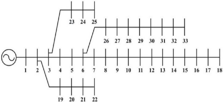
Figure 3 Single-line diagram of the IEEE 33 bus radial distribution system.
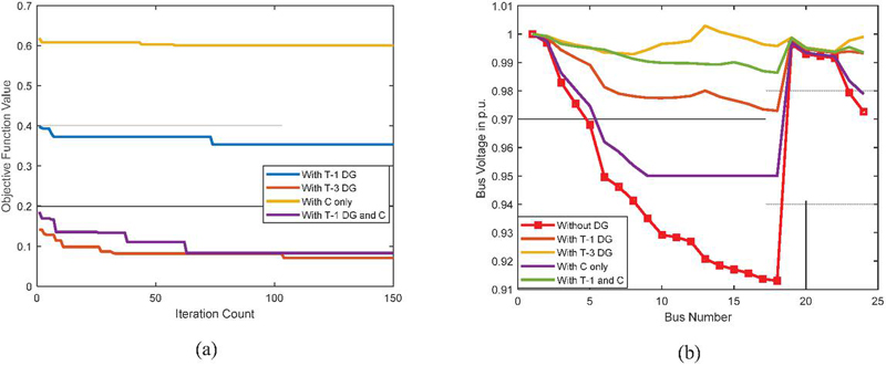
Figure 4 Objective Function characteristics and Bus Voltage Profile for 33 bus system.
Table 2 Comparative study of CPOA for the 33-bus system at full load constant power
| Case | Parameters | CPO Proposed | [25] CTLBO | [19] WIPSO GSA | [15] MFO-SCA | [31] KH |
| 1 | Size MW | 0.82(13) | 0.80(13) | 0.84(13) | 1.05(30) | 0.81(13) |
| (Site) | 1.06(24) | 1.09(24) | 0.86(24) | 1.09(24) | 0.84(25) | |
| 1.08(30) | 1.05(30) | 0.86(30) | 0.80(13) | 0.84(30) | ||
| PL | 71.61 | 72.79 | 74.78 | 72.78 | 75.41 | |
| %RL | 64.66 | 64.08 | 64.56 | 65.5 | 64.25 | |
| 0.969(33) | – | – | 0.9687(33) | 0.961(33) | ||
| TVD | 0.5677 | – | – | – | – | |
| VSI | 0.8819 | 0.8805 | – | – | ||
| Cost($/MWh) | 59.682 | 59.05 | 51.45 | 59.05 | 50.05 | |
| 2 | CPO Proposed | [34] IA | [13] WIPSO GSA | [32] LSFSA | [31] KH | |
| Size | 0.74/0.55(13) | 1.09(6) pf-0.82 lag | 1.02(12) pf-0.85 lead | 1.19/0.69(6) | 0.85/0.49(13) | |
| MW/MVAR | 0.87/0.65(24) | 1.09(30) pf-0.82 lag | 1.03(24) pf-0.84 lead | 0.47/0.27(18) | 0.90/0.51(24) | |
| (Site) | 1.07/0.80(30) | 0.76(14) pf-0.82 lag | 1.08(30) pf-0.8 lead | 0.92/0.53(30) | 0.89/0.51(30) | |
| PL | 14.38 | 22.29 | 16.48 | 26.7 | 19.57 | |
| %RL | 92.90 | 89.45 | 92.19 | 87.34 | 90.72 | |
| 0.9929(8) | – | – | 0.982(25) | 0.9816(33) | ||
| TVD | 0.1204 | – | – | – | – | |
| VSI | 0.9719 | – | – | – | ||
| Cost($/MWh) | 54.23 | 59.05 | 62.85 | 51.85 | 53.05 | |
| 3 | CPO Proposed | [18] EGWO-PSO | [19] WIPSO GSA | [15] MFO-SCA | [39] WCA | |
| Size | 0.44(57) | 0.42(13) | 0.47(12) | 1.00(30) | 0.40(14) | |
| MVAR | 0.66(62) | 0.56(24) | 0.53(29) | 0.33(24) | 0.45(24) | |
| (Site) | 0.33(18) | 1.14(30) | 0.53(30) | 0.38(13) | 1.0 (30) | |
| PL | 121.83 | 132.17 | 141.84 | 138.91 | 130.91 | |
| %RL | 39.88 | 34.79 | 32.78 | 34.16 | 35.40 | |
| 0.95(9) | 0.9377(18) | – | 0.9307(18) | 0.951(18) | ||
| TVD | 1.1529 | – | – | 1.2711 | – | |
| VSI | 0.8145 | 0.775 | – | – | – | |
| Cost($/MWh) | 28.85 | 42.65 | 30.85 | 34.45 | 37.25 | |
| 4 | CPO Proposed | [24] AT | [28] GA | [39] WCA | ||
| Size | 0.57(15)/0.78(30) | NA | 0.12(12) | DG 0.25(16), | 0.56(11)/0.53(14) | |
| MW(Site)/ | 1.27(29)/0.25(10) | 0.24(12) | 0.25(22), 0.5(30) | 0.97(25)/0.46(23) | ||
| MVAR(Site) | 0.83(25)/0.57(26) | SC 0.3(15), 0.3(18), 0.3(29), 0.6(30), 0.3(31) | 1.04(29)/0.56(30) | |||
| PL | 16.83 | 71.93 | 71.25 | 24.69 | ||
| %RL | 91.69 | 63.8 | 64.83 | 87.82 | ||
| 0.9864(18) | 0.9815(8) | 0.971 | 0.980(33) | |||
| TVD | 0.2092 | – | – | – | ||
| VSI | 0.9467 | – | – | – | ||
| Cost($/MWh) | 53.77 | 7.45 | 20.25 | 51.65 |
4.1.2 System with type-III DG incorporation (case 2)
Highest loss reduction of 92.90% is achieved by using the proposed method, which shows better results than previous research paper outcomes. The minimum value of voltage is 0.9929 at bus number 8. Cost is 54.23 $/MWh, which is lower than other compared papers except [15], while [15] gives a high value of active power loss compared to the proposed one.
4.1.3 Incorporation of only the capacitor bank (CB) into the system (case 3)
Power loss and cost for this case using the proposed algorithm are 121.83 kW and 28.85 $/MWh, which is far better than other compared literature. It shows better performance of CPOA. Minimum voltage of value 0.95 is obtained at the 9th bus of the system.
4.1.4 Simultaneous integration of type-I with capacitor bank (case 4)
Though the cost of DG is on the higher side in this case for the proposed method, the loss value is much lower than the others, which is equal to 16.83 KW. It also shows the highest percentage of reduction in loss from the base value. At bus number 18, the value of Vmin is 0.986 p.u.
In the load model consideration, it can be seen that lower values for power losses are obtained when type 3 DG is inserted into the distribution system. But percentage loss reduction is highest in the constant current case, where the loss is reduced from the base case value by 92.53%.
Table 3 Outcomes of the 33-bus system for load models
| Base Case | Unit Size | Unit Size | Unit Size MW[Site]/ | ||||
| Cases | (in kW) | T-1 Only | (MW)/[Site] | T-3 only | (MW/MVAr)/[Site] | T-1 and C | MVAr [Site] |
| CPx0.5 load | 47.07 | 17.070 | 0.59(29), 0.41(13), 0.42(24) | 4.85 | 0.37/0.23(24), 0.38/0.23(15), 0.47/0.29(30) | 6.33 | 0.25(16)/0.17(32), 0.80(6)/0.24(11), 0.33(32)/0.20(29) |
| C Px1.6 load | 575.367 | 164.05 | 1.23(27) 1.40(8) 1.45(24) | 54.39 | 1.42/0.88(25), 1.47/0.91(11), 1.32/0.82(31) | 55.78 | 1.43(13)/1.05(31), 0.87(25)/1.10(4), 1.32(32)/1.08(9) |
| CC | 174.76 | 62.49 | 0.61(14) 0.97(30) 0.95(24) | 13.22 | 0.84/0.52(24), 0.63/0.39(14), 1.20/0.74(30) | 18.34 | 0.56(11)/0.14(9), 1.03(29)/0.60(8), 0.76(24)/0.72(30) |
| CI | 151.10 | 55.03 | 0.77(30) 0.85(25) 0.87(12) | 13.00 | 0.83/0.51(24), 0.86/0.53(30), 0.87/0.54(11) | 15.66 | 0.80(15)/0.42(6) 0.76(25)/0.65(31) 0.84(30)/0.28(17) |
| R | 154.44 | 43.47 | 0.72(13) 1.01(30) 0.86(24) | 12.77 | 0.93/0.58(24), 0.50/0.31(14), 0.97/0.60(30) | 16.64 | 0.84(25)/0.90(3) 0.59(32)/0.62(29) 1.16(10)/0.32(13) |
| C | 157.85 | 48.49 | 0.75(29) 0.73(13) 0.92(25) | 17.16 | 0.38/0.23(17) 0.95/0.59(25) 1.12/0.69(29) | 21.51 | 1.01(30)/0.75(30) 1.09(25)/0.38(18) 0.57(8)/0.45(25) |
| I | 148.79 | 36.30 | 0.76(14) 0.93(30) 0.90(24) | 12.70 | 0.67/0.32(14) 0.97/0.47(30) 1.31/0.63(24) | 16.95 | 0.76(33)/0.56(23) 0.99(11)/0.40(7) 1.41(24)/0.54(31) |
4.2 Test System II-69 Bus Test System
The next test system used is a radial distribution system having 69 nodes with a base voltage of 12.66 kV and a base kVA of 100 MVA, as depicted in Figure 5. For the 69-node RDS, standard line and bus data are referred from Baran and Wu et al. [39]. This system has real and reactive power loads of 3802.19 kW and 2694.6 kVAr. Real and reactive power losses for the base case are 225 kW and 102.16 kVAr, respectively. The minimum value of voltage at bus 65 is 0.909 for the base case.
4.2.1 System with type-I DG incorporation (case 1)
The real power loss obtained by the proposed technique is 70.77 kW which shows 68.54% reduction from the base case. The proposed method gives better results than other literature, as shown in Table 4. Value obtained for Vmin is 1 p.u. at bus number 1. Total voltage deviation (TVD) and voltage stability index obtained are 0.4391 and 0.9163, respectively.
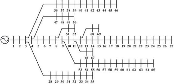
Figure 5 Connection diagram of an IEEE distribution system having 69 buses.
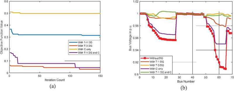
Figure 6 Objective Function characteristics and Bus Voltage Profile for 69 bus
4.2.2 System with type-III DG incorporation (case 2)
Achieved power loss and % loss reduction are 6.87 kW and 96.9434%, which is better than all other research outcomes except [31] and [34]. But the cost from the proposed one is 52.88 $/MWh, which is lower than the above-mentioned papers, which shows a better result in economical point of view. The minimum value of voltage is 0.9926 at bus number 18.
4.2.3 Incorporation of only CB into the system (case 3)
Power loss and cost for this case using the proposed algorithm are 111.99 kW and 28.25 $/MWh, which is far better than other compared literature. It shows better performance of CPOA. Minimum voltage of value 0.95 is obtained at the 58th bus of the system, which is also a better value.
Table 4 Comparative study of CPOA for the 69-bus system at full load constant power
| Case | Parameters | CPO Proposed | [23] IMDE | [1] JAYA-IWO | [32] LSFSA | [33] ECOA |
| 1 | Size | 0.45(18) | 1.73(61) | 0.47(23) | 0.42(18) | 0.74(14) |
| MW | 0.44(11) | 0.473(20) | 0.34(69) | 1.33(60) | 0.65(25) | |
| (Site) | 1.70(62) | 1.71(61) | 0.42(65) | 1.07(30) | ||
| PL | 70.77 | 70.92 | 70.92 | 77.1 | 71.8 | |
| %RL | 68.54 | 68.47 | 68.47 | 65.72 | 68.08 | |
| Vmin | 1.0(1) | 0.9808(65) | 0.979(65) | 0.9811(61) | 0.9784 | |
| TVD | 0.4391 | – | – | – | – | |
| VSI | 0.9163 | – | – | – | – | |
| Cost($/MWh) | 52.29 | 44.31 | 50.65 | 43.65 | 49.45 | |
| 2 | CPO Proposed | [34] IA | [18] EGWO-PSO | [32] LSFSA | [31] KH | |
| Size | 0.69/0.42(10) | 2.07(61) pf-0.82 lag | 0.77(13) | 0.54(18) | 0.56(11) | |
| MW/MVAR | 1.74/1.08(61) | 0.62(17) pf-0.82 lag | 1.07(24) | 1.19(60) | 0.35(22) | |
| (Site) | 0.19/0.12(25) | 0.82(50) pf-0.82 lag | 1.03(30) | 0.31(65) | 1.77(61) | |
| PL | 6.87 | 4.95 | 11.68 | 16.26 | 5.92 | |
| %RL | 96.9434 | 97.74 | 94.24 | 92.76 | 92.8 | |
| Vmin | 0.9926(18) | – | 0.9926(8) | 0.9885(61) | 0.9943(50) | |
| TVD | 0.1542 | – | – | – | – | |
| VSI | 0.9707 | – | 0.9707 | – | 0.9772 | |
| Cost($/MWh) | 52.88 | 70.45 | 57.65 | 41.05 | 53.85 | |
| 3 | CPO Proposed | [23] IMDE | [18] EGWO-PSO | [35] PVSC, DGPI | [21] WCA | |
| Size | 0.44(57) | 1.26(61) | 0.42(11) | 0.35(50) | 1.28(61) | |
| MVAR | 0.66(62) | 0.37(21) | 0.25(20) | 1.05(61) | 0.21(69) | |
| (Site) | 0.33(18) | 1.41(61) | 0.39(64) | 0.27(18) | ||
| PL | 111.99 | 145.53 | 145.13 | 66.74 | 144.53 | |
| %RL | 50.21 | 35.2 | 35.5 | 33 | 28.68 | |
| Vmin | 0.95(58) | 0.9330(65) | 0.9314(65) | 0.97 | 0.95(65) | |
| TVD | 1.3282 | – | – | – | 0.698 | |
| VSI | 0.8145 | – | 0.7841 | – | 0.961 | |
| Cost($/MWh) | 28.25 | 32.85 | 41.85 | 36.05 | 35.45 | |
| 4 | CPO Proposed | [23] IMDE | [36] Fuzzy GA | [35] PVSC, DGPI | [21] WCA | |
| Size | 0.69(17)/0.17(21) | 1.73(62)/0.10(63) | 1.58/1.13 | 1.85/1.79 | 0.54(17)/1.18(2) | |
| MW(Site)/ | 0.20(50)/1.10(61) | 0.47(24)/1.19(61) | 2(61)/1.23(62) | |||
| MVAR(Site) | 1.70(62)/0.06(69) | 1.15(69)/0.26(69) | ||||
| PL | 10.05 | 13.83 | 19.18 | 9.63 | 33.33 | |
| %RL | 95.53 | 93.84 | 91.47 | 91 | 85.18 | |
| Vmin | 0.9948(50) | 0.9915(68) | 0.9859(65) | 0.99 | 0.994(50) | |
| TVD | 0.0759 | – | – | – | 0.0071 | |
| VSI | 0.9795 | – | 0.9846 | – | 0.965 | |
| Cost($/MWh) | 52.39 | 44.25 | 31.94 | 37.25 | 74.25 |
4.2.4 Simultaneous integration of type-I with capacitor bank (case 4)
The percentage reduction in power loss obtained by the proposed algorithm is 95.53%, which shows the best performance of the proposed technique compared to previous literature shown in the table. It also shows the highest percentage of reduction in loss from the base value. Though the cost of DG is on the higher side in this case for the proposed method, the loss value is much lower than the others, which is equal to 10.05 kW except [35]. At bus number 50, the value of Vmin is 0.9948 p.u.
Table 5 Outcomes of the 69 bus RDS with load models
| Cases | |||||||
| Base Case | Unit Size | Unit Size | Unit Size MW[Site]/ | ||||
| Load Model | (in kW) | T-1 Only | (MW)/[Site] | T-3 only | (MW/MVAr)/[Site] | T-1 and C | MVAr [Site] |
| CPx0.5 load | 51.59 | 18.22 | 0.80(61) 0.46(3) 0.46(13) | 2.74 | 0.41/0.31(12) 0.87/0.65(61) 0.23/0.17(46) | 6.71 | 0.75(64)/0.82(3) 0.27(38)/0.74(63) 0.38(13)/0.46(29) |
| C Px1.6 load | 652.41 | 172.85 | 0.79(17) 0.91(55) 1.19(56) | 36.57 | 0.82/0.61(14) 1.19/0.89(61) 1.01/0.75(62) | 70.52 | 0.58(21)/1.00(63) 1.03(64)/0.07(54) 1.12(62)/0.90(12) |
| CC | 188.60 | 63.30 | 1.08(62) 0.56(13) 0.51(64) | 8.16 | 1.18/0.89(61) 0.35/0.26(16) 0.32/0.24(63) | 13.7 | 0.55(14)/1.10(51) 0.95(64)/0.34(19) 0.75(61)/0.83(61) |
| CI | 158.74 | 52.81 | 0.40(64) 1.08(61) 0.41(21) | 7.50 | 0.32/0.24(57) 0.48/0.36(16) 1.16/0.87(62) | 12.62 | 0.98(60)/1.13(61) 0.57(12)/1.61(11) 0.56(64)/0.96(34) |
| R | 164.82 | 43.84 | 0.91(63) 0.97(12) 0.68(58) | 12.18 | 0.52/0.39(20) 1.14/0.85(61) 0.85/0.63(49) | 13.05 | 1.11(61)/0.93(61) 0.32(68)/0.12(5) 0.48(18)/0.57(12) |
| C | 156.88 | 43.80 | 0.49(64) 0.91(61) 0.58(16) | 7.28 | 0.33/0.25(21) 1.19/0.89(61) 0.63/0.47(66) | 12.31 | 0.61(58)/0.69(61) 0.84(62)/0.16(17) 0.55(15)/0.55(60) |
| I | 173.3384 | 44.52 | 0.89(33) 0.49(72) 0.61(11) | 15.37 | 1.08/0.81(9) 0.32/0.24(73) 0.60/0.45(35) | 15.91 | 0.59(31)/0.17(14) 0.52(79)/0.39(33) 0.61(26)/0.47(63) |
4.3 Test System III: 85-Bus Radial Distribution Network
In Figure 8, the single-line diagram of the 85-bus network is given. For the line and bus data, [16] is referred to as an 85-bus standard test system having 85 nodes and 84 branches. 12.66 kV and 100 MVA, respectively, are the values of base voltage and base kVA in this system. This system has active and reactive power of the loads are 2.5703 MW and 2.6222 MVAr. In the base case, active and reactive power losses are 316 kW and 198.57 kVAr, respectively.
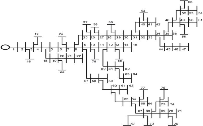
Figure 7 Single-line diagram of radial network having 85 buses.
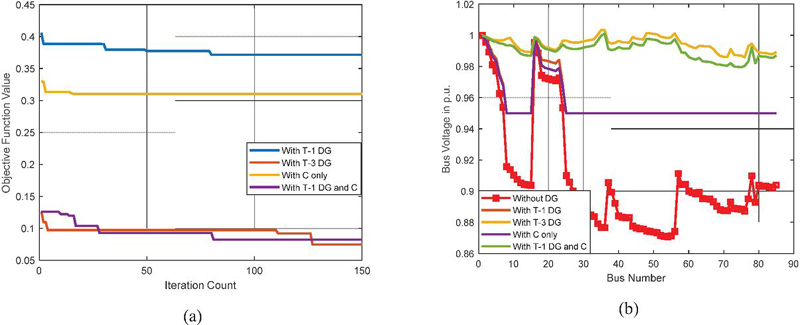
Figure 8 Objective Function characteristics and Bus Voltage Profile for 85 bus.
4.3.1 System with type-I DG incorporation (case 1)
The real power loss obtained by the proposed technique is 117.43 kW which shows 62.85% reduction from the base case. The proposed method gives the best result in terms of power loss reduction than other literature. Value of obtained cost is 34.93 $/MWh, which also shows better result than other papers except [17]. But power loss is very high in [17]. So the proposed method shows better performance.
Table 6 Comparative study of CPOA for the 85-bus system at full load constant power
| Case | Parameters | CPO | [37] AQIEA | [17] WOA | [19] WIPSO GSA | [20] MFF |
| 1 | Size | 1.10(7) | 0.68(66) | 0.94(55) | 0.59(26) | 1.0(9) |
| MW/ | 0.36(3) | 0.95(25) | 0.60(34) | 0.70(33) | ||
| (Site) | 0.26(23) | 0.64(34) | 0.59(67) | 0.50(61) | ||
| PL | 117.43 | 151.89 | 224.04 | 152.38 | 151.79 | |
| %RL | 62.85 | 51.95 | – | 51.07 | 51.86 | |
| Vmin | 0.95(8) | – | 0.9109 | – | 0.9435 | |
| TVD | 3.68 | – | – | – | – | |
| VSI | 0.81 | – | – | – | 0.7923 | |
| Cost($/MWh) | 34.93 | 45.65 | 19.05 | 35.85 | 44.25 | |
| 2 | Size | 0.76/0.57(35) | NA | 1.289(55) | 0.89(26) | NA |
| MW/MVAR | 1.18/0.89(9) | 0.85(35) | ||||
| (Site) | 0.4/0.3(64) | 0.89(64) | ||||
| PL | 23.98 | 157.485 | 20.19 | |||
| %RL | 92.54 | 50.11 | 93.52 | |||
| Vmin | 0.9858(78) | 0.9255 | – | |||
| TVD | 0.4698 | – | – | |||
| VSI | 0.9446 | – | – | |||
| Cost($/MWh) | 47.39 | 26.03 | 52.85 | |||
| 3 | [38] PSO | [17] WOA | [19] WIPSO GSA | [20] MFF | ||
| Size | 0.83(7) | 1.04(9) | DGII- | 0.60(25) | 1.00(9) | |
| MVAR | 0.36(35) | 0.67(34) | 0.87(55) | 0.60(35) | 0.70(33) | |
| (Site) | 0.40(60) | 0.56(64) | 0.60(67) | 0.45(61) | ||
| PL | 98.05 | 151.19 | 229.02 | 153.79 | 154.06 | |
| %RL | 68.98 | 52.17 | 27.45 | 50.62 | 51.15 | |
| Vmin | 0.95(8) | – | 0.903 | – | 0.9171 | |
| TVD | 3.72 | – | – | – | – | |
| VSI | 0.81 | – | – | – | 0.7074 | |
| Cost($/MWh) | 32.05 | 45.65 | 17.65 | 36.25 | 43.25 | |
| 4 | [40] GABC | [19] WIPSO GSA | [29] SSO | |||
| Size | 0.47(10)/0.73(9) | 0.57(36)/0.3(53) | NA | 0.50(27)/0.43(29) | 0.95(9)/0.94(9) | |
| MW(Site)/ | 0.69(36)/0.77(36) | 1.20(56)/0.45(46) | 0.50(35)/0.45(36) | 0.7(33)/0.72(33) | ||
| MVAR(Site) | 0.80(57)/0.51(69) | 0.42(54)/0.3(54) | 0.50(67)/0.51(67) | 0.47(61)/0.50(61) | ||
| PL | 25.99 | 73.24 | 37.27 | 20.98 | ||
| %RL | 91.77 | 76.85 | 88.21 | 93.35 | ||
| Vmin | 0.9795(75) | 0.9612 | 0.964 | 0.9855 | ||
| TVD | 0.812 | 2.3139 | – | – | ||
| VSI | 0.920 | 0.8546 | – | 0.9431 | ||
| Cost($/MWh) | 39.76 | 44.05 | 30.25 | 42.65 |
Table 7 Results of 85 bus RDN with Load Model
| Cases | |||||||
| Base Case | Unit Size | Unit Size | Unit Size MW[Site]/ | ||||
| Load Model | (in kW) | T-1 Only | (MW)/[Site] | T-3 only | (MW/MVAr)/[Site] | T-1 and C | MVAr [Site] |
| CP x0.5 load | 66.54 | 34.50 | 1.07[68,9,49] | 5.79 | 1.23/0.94 [67, 32, 9] | 8.17 | 1.0 [48, 26, 8]/ 0.99 [80, 59, 42] |
| C Px1.6 load | 932.25 | 243.47 | 2 [7, 58, 6] | 69.33 | 3.25/2.44 [34, 67, 82] | 75.25 | 2.67[49, 26, 65]/ 3.12[68, 49, 59] |
| Constant Current | 233.32 | 107.99 | 1.15 [20, 60, 7] | 20.71 | 1.94/1.45 [34, 26, 64] | 28.05 | 2.42[67, 32, 46]/ 1.72[72, 7, 33] |
| Constant Impedance | 182.74 | 92.00 | 1.65 [65, 9, 31] | 17.77 | 1.72/1.29 [32, 8, 67] | 20.56 | 1.68[34, 8, 55]/ 1.71[77, 57, 36] |
| Residential | 175.13 | 62.03 | 1.96 [72, 8, 35] | 11.53 | 1.7/1.27 [67, 12, 32] | 17.69 | 1.67[32, 31, 60] / 1.44[70, 9, 32] |
| Commercial | 168.53 | 69.66 | 1.66[64, 9, 36] | 12.23 | 1.81/1.36 [11, 64, 31] | 17.44 | 1.81[55, 63, 9]/ 1.24[67, 59, 49] |
| Industrial | 173.84 | 47.50 | 1.89[49, 12, 72] | 14.48 | 1.9/1.42 [32, 64, 9] | 15.91 | 1.72[31, 79, 2]/ 1.03[14, 33, 63] |
4.3.2 System with type-III DG incorporation (case 2)
Highest loss reduction, i.e. 92.54% is achieved by using the proposed method, which shows better results than previous research paper outcomes. The minimum value of voltage is 0.858 at bus number 78. Cost is 47.39 $/MWh, which is lower than other compared papers except [17], while [17] gives a huge value of active power loss compared to the proposed one.
4.3.3 Incorporation of only the capacitor bank into the system (case 3)
Power loss for this case using the proposed algorithm is 98.05 kW, which is far better than other compared literature. It shows better performance of CPOA. Minimum voltage of value 0.95 is obtained at the 8th bus of the system. Total voltage deviation (TVD) and voltage stability index obtained are 3.72 and 0.81, respectively.
4.3.4 Simultaneous integration of type-I with a capacitor bank (case 4)
Though the cost obtained by the proposed method, i.e. 39.76 $/MWh is on the higher side than [19], the achieved loss by the proposed algorithm is far better than [19], which is equal to 25.99 kW. At bus number 75, the value of Vmin is 0.9795 p. u. Total voltage deviation and VSI obtained are 0.812 and 0.920, respectively.
The various load models are studied for individual DG integration and the optimal simultaneous DG and capacitor placement. Tables 3, 5 and 7 represent the line losses for various load models for bus systems I, II, and III, respectively, except the constant power (full load) model. Figures 3, 6 and 9 represent the objective function for all three-bus system i.e. 33 bus, 69 bus and 86 bus systems. Likewise Figures 4, 7 and 10 represent the voltage profile for all three-bus system i.e. 33 bus, 69 bus and 86 bus systems.
5 Conclusion
In this article, CPOA shows better results in achieving the desired objective function in a successful manner for optimal placement of compensating units. The efficacy of the method is tested on various load models, and the results are verified with the previous research articles. The power losses are minimized effectively, and voltages are also improved over buses. TVD and VSI are also calculated and found effective. The cost for a total number of units is calculated and compared to many previous methods, and it is found to be lesser. Moreover, the proposed methodology presents an electrically and economically viable solution for the optimal placement of DGs, switched capacitors, and the simultaneous operation of the two. The application of the proposed method and likely algorithms to an unstable system could be the future scope of the work.
References
[1] N. Saxena, M. Pandit, L. Shrivastava, “Novel JAYA-IWO Approach for Optimal Distributed Generation Placement to minimize Power Losses”, The Social and Ethical Implications of Nanotechnology and Engineering, 20, S4, https://doi.org/10.62441/nano-ntp.vi.642, 2024.
[2] Thai Dinh Pham, Thang Trung Nguyen, Kien Le C., “An Improved Equilibrium Optimizer for Optimal Placement of Distributed Generators in Distribution Systems Considering Harmonic Distortion Limits”, Research Square, 2022.
[3] Shah Danish S. M., Ahmadi, M., Atsushi, Y., Tomonobu, S., Narayanan, K., Hiroshi, T., “Multi-objective optimization of optimal capacitor allocation in radial distribution systems”. International Journal of Emerging Electric Power Systems, 2020.
[4] Eid A., “Allocation of distributed generations in radial distribution systems using adaptive PSO and modified GSA multi-objective optimizations”. Alexandria Engineering Journal, 2020, 59, 4771–4786.
[5] Mohd Tauseef Khan, Pushpendra Singh, Anurag Chauhan, Rajesh Arya, Anchal Verma, Titare, L. S., Choube, S.C., “Optimal placement of multiple distributed generators using a novel voltage stability indicator employing arithmetic optimization algorithm”. Computer and Electrical Engineering, 2023,110, 1088853, 0045-7906.
[6] Saxena, N., Pandit, M., Srivastava L., “Multi-objective DG placement in radial distribution systems using the IbI logic algorithm”. Front. Energy Res. 2024, 12:1453715.
[7] Rajmistry, S., Titare, L.S., “A novel approach for allocation of optimal capacitor and distributed generation on radial distribution system”. Int. Journal of Recent Research in Elect. And Electronics Engg., 2015, 2,3, pp. 126–134.
[8] Gholami, K., Parvaneh, M. H., “A mutated salp swarm algorithm for optimum allocation of active and reactive power sources in radial distribution systems”. Applied Soft Computing, 2019, 85, 105833, 1568–4946.
[9] Naderipour, A., Abdul-Malek, Z., Hajivand, M., Seifabad, Z. M., Farsi, Ali Farsi M., Nowdeh, S. A., Davoudkhani I. F., “Hyena optimizer algorithm for capacitor allocation in radial distribution system with distributed generation and microgrid operation considering different load types”. Scientific reports, 2021, 11.
[10] Abdel–mawgoud, H., “Optimal Allocation of DG and Capacitor in Distribution Network Using a Novel Hybrid MFO-SCA Method”, Electric Power Components and Systems, 2021.
[11] Pham, Thai, Nguyen, Thang and Dinh, Bach, “Find optimal capacity and location of distributed generation units in radial distribution networks by using enhanced coyote optimization algorithm”. Neural Computing and Applications. 2021, 33.
[12] Bohre, A.K., Agnihotri, G., Dubey, M., “Optimal sizing and siting of DG with load models using soft computing techniques in practical distribution system”. IET Generation, Transmission & Distribution, 2016, 1–16, 1751–8687.
[13] Prakash R., Lokeshgupta B., “Optimal site and size of DG with different load model using Cuckoo search algorithm”. IEEE, 2018.
[14] Bouchekara, Houssem, “Comprehensive Review of Radial Distribution Test Systems”. ResearchGate, 2020.
[15] Baran M. E., Wu F. F., “Network reconfiguration in distribution systems for loss reduction and load balancing”. IEEE Transactions on Power Delivery, 1989, 4, 2, 1401–1407.
[16] Priyanka Patil, Usha Surendra, “Potential Drop Analysis of a Radial Distribution System with Various Loads”. International Journal of Innovative Technology and Exploring Engineering (IJITEE), 2278–3075, 9(5).
[17] Prasad Reddy P. D., Veera Reddy V. C., Manohar, T. G., “Whale optimization algorithm for optimal sizing of renewable resources for loss reduction in distribution systems”. Renewables: Wind, Water, and Solar, 2017,4:3.
[18] Venkatesan, C., Kannadasan, R., Alsharif, M.H., Kim, M.-K., Nebhen, J., “A Novel Multi objective Hybrid Technique for Siting and Sizing of Distributed Generation and Capacitor Banks in Radial Distribution Systems”. Sustainability, 2021, 13, 3308
[19] Rajendran, A., Narayanan, K., “Optimal multiple installation of DG and capacitor for energy loss reduction and loadability enhancement in the radial distribution network using the hybrid WIPSO–GSA algorithm”. International Journal of Ambient Energy, 2018, 41(2), 129–141.
[20] Sukraj, K., Yuvaraj, T., Hariharan, R., Thirumalai, M., “Simultaneous Allocation of Shunt Capacitor and Distributed Generator in Radial Distribution Network Using Modified Firefly Algorithm”. International Conference on Smart Structures and Systems (ICSSS), Chennai, India, 2019, 1–5.
[21] El-Ela, A. A. A., El-Sehiemy R. A., Abbas, A. S., “Optimal Placement and Sizing of Distributed Generation and Capacitor Banks in Distribution Systems Using Water Cycle Algorithm”. IEEE Systems Journal, 2018, 12, 4, 3629–3636.
[22] Biswal, S. R., Shankar, G., “Optimal deployment and sizing of distributed generations and capacitor banks in radial distribution system using African vultures optimization algorithm”. AIP Conference Proceedings, 2022, 2681, 02007.
[23] Khodabakhshian A., Mohammad Hadi Andishgar, “Simultaneous placement and sizing of DGs and shunt capacitors in distribution systems by using IMDE algorithm”. International Journal of Electrical Power & Energy Systems, 2016, 82, 599–607, ISSN 0142-0615.
[24] S. Gopiya Naik, D. K. Khatod, M.P. Sharma, “Optimal allocation of combined DG and capacitor for real power loss minimization in distribution networks”, Electrical Power and Energy Systems, 53, 967–973, (2013).
[25] Quadri, Imran, Bhowmick, S., Joshi, Dheeraj. (2018), “A comprehensive technique for optimal allocation of distributed energy resources in radial distribution systems”. Applied Energy. 211. 1245–1260. doi:10.1016/j.apenergy.2017.11.108.
[26] Imran Ahmad Quadri, S. Bhowmick, D. Joshi, “A comprehensive technique for optimal allocation of distributed energy resources in radial distribution systems”, Applied Energy, 211, 1245–1260, ISSN:0306-2619, https://doi.org/10.1016/j.apenergy.2017.11.108, (2018).
[27] Mohamed Abdel-Basset, Reda Mohamed, Mohamed Abouhawwash, “Crested Porcupine Optimizer: A new nature-inspired metaheuristic”, Knowledge-Based Systems, 284, 111257, ISSN: 0950-7051, https://doi.org/10.1016/j.knosys.2023.111257, (2024).
[28] A. K. Saonerkar and B. Y. Bagde, “Optimized DG placement in radial distribution system with reconfiguration and capacitor placement using genetic algorithm,” 2014 IEEE International Conference on Advanced Communications, Control and Computing Technologies, Ramanathapuram, India, 2014, pp. 1077–1083, doi:10.1109/ICACCCT.2014.7019263.
[29] N. Gnanasekaran, S. Chandramohan, P. Sathish Kumar, A. Mohamed Imran, “Optimal placement of capacitors in radial distribution system using shark smell optimization algorithm, Ain Shams Engineering Journal, Volume 7, Issue 2, 2016, Pages 907–916, ISSN 2090-4479, https://doi.org/10.1016/j.asej.2016.01.006.
[30] Guerraiche, Khaled, Belballi, Abdelatif, G�ven, Aykut, Dekhici, Latifa and Abbou, Amine. (2025), “Cheetah Optimization for Optimal Sizing and Placement of Distributed Generation and Capacitors”. Jordan Journal of Electrical Engineering. 11. 1. doi:10.5455/jjee.204-1733161680.
[31] Sneha Sultana, Provas Kumar Roy, “Krill herd algorithm for optimal location of distributed generator in radial distribution system”, Applied Soft Computing, vol. 40, pp. 391–404, ISSN: 1568-4946, https://doi.org/10.1016/j.asoc.2015.11.036, (2016).
[32] Satish Kumar Injeti, N. Prema Kumar, “A novel approach to identify optimal access point and capacity of multiple DGs in a small, medium and large scale radial distribution systems”, International Journal of Electrical Power & Energy Systems, 45(1), 142151, ISSN 0142, 0615, https://doi.org/10.1016/j.ijepes.2012.08.043, (2013).
[33] Pham, Thai, Nguyen, Thang and Dinh, Bach, “Find optimal capacity and location of distributed generation units in radial distribution networks by using enhanced coyote optimization algorithm”. Neural Computing and Applications 33, doi:10.1007/s00521-020-05239-1, (2021).
[34] D. Q. Hung and N. Mithulananthan, “Multiple Distributed Generator Placement in Primary Distribution Networks for Loss Reduction,” in IEEE Transactions on Industrial Electronics, vol. 60, no. 4, pp. 1700–1708, April 2013, doi:10.1109/TIE.2011.2112316.
[35] Nawaz, S., Bansal, A., Sharma, M, “Optimal Allocation of Multiple DGs and Capacitor Banks in Distribution Network”. European Journal of Scientific Research. 2016, 142.
[36] Gampa, S.R., Das, D, “Simultaneous optimal allocation and sizing of distributed generations and shunt capacitors in distribution networks using fuzzy GA methodology”. Journal of Electrical Systems and Inf Technol 6, 2019, 4. https://doi.org/10.1186/s43067-019-0003-2.
[37] Kanta, G Mani, Mani, Ashish, Singh, H.P. and Chaturvedi, “Effect of Voltage-Dependent Load Model on Placement and Sizing of Distributed Generator in Large Scale Distribution System”, Majlesi Journal of Electrical Engineering, 14, 97–121, doi:10.29252/mjee.14.4.97, (2020).
[38] G. E. Mendoza, V. M. Vacas and N. R. Ferreira, “Optimal Capacitor Allocation and Sizing in Distribution Networks Using Particle Swarm Optimization Algorithm,” Workshop on Communication Networks and Power Systems (WCNPS), Bras�lia, Brazil, 1–5, doi:10.1109/WCNPS.2018.8604320, (2018)
[39] Baran M. E., “Wu F. F. Optimal capacitor placement on radial distribution systems”. IEEE Transactions on Power Delivery, 1989, 4,1, 725–734.
[40] Mukul Dixit, Prasanta Kundu, Hitesh R. Jariwala, “Incorporation of distributed generation and shunt capacitor in radial distribution system for techno-economic benefits”, Engineering Science and Technology, an International Journal, 20, 2, 2017, 482–493, ISSN 2215-0986, https://doi.org/10.1016/j.jestch.2017.01.003.
Biography

Shilpa Phatak received the bachelor’s degree in electrical engineering from CSVTU in 2010, the master’s degree in High voltage from RGPV Bhopal in 2014, respectively and pursuing the philosophy of doctorate degree from RGPV Bhopal. Her research areas include power system, renewable energy sources, smart grid etc.
Strategic Planning for Energy and the Environment, Vol. 45_3, 1007–1034
doi: 10.13052/spee1048-5236.45314
© 2026 River Publishers