Optimised PIDN–FACTS Control for Frequency Stability in Multi-Area Systems with Fuel Cell Integration
Vivek Kaushal Lawyee1,*, Loveleen Kaur Taneja1, Ajay Kumar1 and Shimi S. L.2
1Punjab Engineering College (Deemed To Be University), Chandigarh, India
2Indian Naval Academy, Ezhimala, Kannur, Kerala, India
E-mail: lawyee.vivek@gmail.com; loveleenkaur@pec.edu.in; ajaykumar@pec.edu.in; shimi.1980@navy.gov.in
*Corresponding Author
Received 30 September 2025; Accepted 05 January 2026
Abstract
The growing induction of renewable and cleaner energy sources has made present-day interconnected power grids more complex, where frequency stability and tie-line power control are significant issues. This work presents a realistic two-area interconnected system modelled in MATLAB/Simulink comprising gas, reheat-thermal, and hydro units, with nonlinear consideration and a modified Proportional-Integral-Derivative-Filter (PIDN) controller design. The impact of the inclusion of a Fuel Cell (FC) unit with the grid on frequency stability is analysed, and a coordinated control strategy with Flexible AC Transmission System (FACTS) devices is developed. Several FACTS devices, namely Thyristor Controlled Series Capacitor (TCSC), Unified Power Flow Controller (UPFC), Interline Power Flow Controller (IPFC), and Static Synchronous Series Compensator (SSSC), are designed and integrated with the grid to improve frequency stability. Three population-based optimisation algorithms, viz, Grey Wolf Optimisation (GWO), Artificial Bee Colony (ABC), and Differential Evolution (DE), are used for minimising the cost function, Integral of Time multiplied by Absolute Error (ITAE), for optimal tuning of PIDN and FACTS controllers. A comprehensive study is performed across four scenarios, including single-area and multi-area Step Load Perturbations (SLP). The control performance of each strategy is evaluated based on the obtained ITAE, settling times, peak overshoots, peak undershoots, and rise times. Results demonstrate that GWO outperforms ABC and DE by achieving better control dynamics. Moreover, inclusion of FC achieves a substantial reduction in ITAE compared to conventional approaches, with values as low as 0.002044. FACTS devices further enhance performance, with IPFC consistently achieving the best damping, lowering ITAE to nearly half of the baseline PIDN–GWO values in multi-area disturbances. Overall, the study establishes that coordinated deployment of optimised controllers, FACTS technologies, and cleaner energy sources can significantly strengthen frequency regulation.
Keywords: Fuel cell, flexible AC transmission system, grey wolf optimisation, artificial bee colony, differential evolution, integral of time multiplied by absolute error.
1 Introduction
1.1 Background
The reliability and stability of power systems are heavily dependent on their ability to maintain nominal frequency despite continuous and unpredictable load variations. As the electrical power generated must always match the demand in real-time, any imbalance leads to frequency deviations, which, if not promptly corrected, can compromise system integrity and operation [1]. This challenge is addressed by Automatic Generation Control (AGC), a critical component in modern power systems that automatically regulates the generation of multiple generating units to maintain frequency and tie-line power flow. The function of AGC is widely acknowledged as Load Frequency Control (LFC), a process that becomes even more complex in multi-area interconnected systems due to inter-area power flows and dynamic interactions [2, 3]. For the study of LFC of interconnected areas, accurate modelling of the power system is essential. This requires a precise mathematical exemplification of the generating units that form part of an actual power system [4]. These units must be modelled while considering practical restrictions such as Generation Rate Constraint (GRC) and Governor Dead Band (GDB) [5, 6]. GRC defines the realistic bounds of power generation due to the physical constraints of the turbine, while GDB represents a delay in the system’s response to act upon change [7]. Furthermore, modern smart grids achieve frequency control with the help of signals received from various Phasor Measurement Units (PMUs) spread across a wide area. Therefore, the effects of data sampling and communication delays must also be considered in a practical smart power system model [8, 9].
1.2 Literature Review
LFC in an interconnected grid has evolved from the analysis of single-area systems to more complex multi-area configurations. Numerous studies have been done focusing on two-area, three-area [10], and four-area [11] interconnected systems to represent a power system with multiple utility regions. The purpose of representing a multi-area power system for LFC studies is to consider the dynamics of interconnected areas while incorporating tie-line power exchanges. While considering more interconnected areas increases the practicality of the situation, it makes the grid model more intricate. Considering this fact, most of the studies focus on a two-area interconnected grid as it allows tie line exchanges without complicating the model.
The composition of the power grid across the globe is changing constantly with the amalgamation of several renewable energy sources (RES). Several researchers have focused on this changing composition and have considered hybrid power systems for their frequency control, for instance, in [12], a multi-microgrid system has been considered for frequency control. Similarly, a renewable source integrated power system has been considered in [13]. This study incorporates Solar and wind power plants with conventional thermal units in an interconnected grid. In [14], a wind energy source with Electric Vehicle (EV) aggregation has been considered for LFC studies. EVs could help in providing the frequency support during critical load variations due to the availability of stored energy in their batteries. Several other researchers have also considered Plug-in Hybrid Electric vehicles integrated with the conventional power system for improvement of frequency regulation [15, 16].
Energy Storage Systems (ESS) like batteries, flywheels, Fuel Cells (FCs) and super capacitors have flourished recently for their several benefits in power systems. These sources store energy during excess generation in the power system and supply during a shortfall of energy, hence supporting frequency. Along with ESS, High Voltage DC (HVDC) links also help in regulating frequency. HVDC link with an AC tie line introduces power electronic converters, which can control power flow. The effect of incorporating Vanadium redox flow battery (VRFB) and Super Magnetic Energy Storage System (SMES) along with HVDC link on power system frequency stability is studied in [17]. In [18], the authors investigated the impact of the inclusion of FC on damping frequency variations. In addition to these devices, Flexible AC Transmission Systems (FACTS) devices can regulate real and reactive power flowing through transmission networks using power electronics controllers. Some studies have explored the use of several FACTS devices like TCSC [19] and UPFC [20] in frequency regulation and control of the power system.
LFC primarily alters the generator’s output with the help of speed governors, which alter the mechanical power input to the turbine depending upon frequency changes. Further, the Integral controller is used to eliminate the Area Control Error (ACE) and bring the frequency to the nominal level. Several controllers other than integral have also been explored in the literature, like Proportional Integral Derivative (PID) controller [21], Fuzzy-PIDF [22], Fractional Order Integral-Tilt Derivative with Filter (FOI-TDN) [23], 2-DOF-PID-FOI [24]. Some other studies focused on developing different control architectures by designing controllers with a High-order differential feedback controller [25], a second-order Sliding Mode Control (SMC) via double-integrated sliding surface [26], a multi-phase SMC scheme [27], Adaptive High-Order Sliding Mode Control (HOSMC) [28] and a mixed H2/H8 robust control scheme [29]. Among all these controllers, the PID controller is still the simplest and most widely adopted controller. However, conventional PID shows limitations in handling nonlinearities, delays, and rapidly changing operating conditions in modern power networks. Therefore, in this research, a modified PID controller is used, which combines conventional PID with a low-pass filter cascaded with the derivative part and an anti-windup saturation block with the integral controller. This helps in improving its performance, noise immunity and makes it robust for more practical nonlinear systems.
Moving further from controller design, another aspect of effective stability control is the choice of optimisation method. Several optimisation techniques, such as Artificial Rabbits Optimisation (ARO) [30], Archimedes optimization algorithm (AOA) [31], Artificial Bee Colony (ABC) [32], Differential Evolution (DE) [33], Firefly Algorithm (FA) [33], Hunger Games Search Algorithm (HGS) [34] and Innate-Oriented Largescale Multi-agent Double Delayed DDPG (IOLS-MA4DPG) [35] have been implemented to both conventional LFC structure and restructuring power system network. The role of these optimisation procedures is to reduce the cost function, which consists of the rate of change of frequency (ROCOF) in different areas of a multi-area network, and to minimise tie-line power exchanges. Hence, these techniques provide optimum values of several controllable parameters of the grid for effective power system operation and control. In continuation, several studies have explored newer perspectives on this problem. For instance, the impact of Variable Frequency Transformer (VFT) on frequency stabilisation of a multi-area power system network is investigated in [36] and [37]. Similarly, Ref. [38] implemented demand response in LFC using active disturbance rejection control, while Ref. [39] presented a model-free output feedback (OPFB) approach to address the LFC problem.
1.3 Motivation and Contribution
Inspired by the proven effectiveness, wide applicability and simple design of the PID controller, a modified PID controller structure is developed and incorporated for this study. The modified design incorporates a low-pass filter with the derivative part to suppress noise, and anti-windup protection with the integral term to enhance reliability under nonlinear operating conditions. Besides this, most existing studies which have examined the use of FACTS devices for improving stability and control have primarily focused on individual controllers, without providing a comprehensive comparison of different alternatives. Therefore, this study targets to highlight the necessity of a supplementary damping controller to mitigate frequency oscillations and provides a systematic comparative analysis of multiple FACTS devices, including SSSC, TCSC, IPFC, and UPFC. Further motivated by the strong push all around the globe for cleaner and efficient energy sources, this study investigates the role of FC on the frequency oscillations when incorporated with these FACTS devices and the conventional power grid. In addition to this, optimisation algorithms such as Grey Wolf Optimisation (GWO), ABC, and DE have been implemented in this work to ensure optimal tweaking of the controller and FACTS parameters is achieved. The essential contributions of this research are outlined below:
1. Design and development of a modified PID controller incorporating derivative filtering and anti-windup protection for integration with a multi-source interconnected grid, considering non-linearities.
2. Systematic comparative analysis of multiple FACTS devices (SSSC, TCSC, IPFC, and UPFC) for enhancing stability in an interconnected grid.
3. This study presents a novel framework that combines FC-based generation with FACTS devices in a conventional grid, focusing on their synergistic role in improving frequency stability.
4. Application of modern optimisation algorithms such as GWO, ABC, and DE for optimal tuning of the controller and FACTS parameters.
5. Performance evaluation under various load perturbation scenarios and FC integration scenario with the Integral of Time-Multiplied Absolute Error (ITAE) employed as the performance index.
1.4 Organisation of Work
The rest of the research article is documented as follows: Section 2 describes the interconnected power system, which is under research for this study, consisting of a reheat thermal, a gas and a hydro power plant in two areas of the power system followed by modelling of various FACTS devices like SSSC, TCSC, IPFC, UPFC and FC model. Section 3 discusses the designed control architecture for LFC studies, including modified PID design, objective function formulation and optimisation algorithms like GWO, ABC, and DE. Section 4 highlights various simulation results under various load scenarios, and scenarios with the inclusion of FC with the conventional power grid. The study concludes in Section 5, where potential directions for future work are also proposed.
2 System Description and Modelling
2.1 Interconnected Grid Model
The system under consideration for LFC studies is a diverse-source two-area interconnected grid comprising a reheat-thermal, a gas unit, and a hydro unit in each area, as illustrated in Figure 1. Each area of this power system is designed to have a rated power of 2000 MW and a nominal load of 1740 MW. This load is shared among the reheat-thermal (1000 MW), hydro (500 MW), and gas (240 MW) units, resulting in participation factors of 0.5747, 0.2873, and 0.138, respectively. For the representation of different components of each power plant unit, such as the governor, turbine, droop, and valve positioner, transfer function modelling is used, and their parameter values are provided in Table A.1 in Appendix [31]. Additionally, for a practical representation of the power system, several nonlinearities, including GRC and GDB, have also been considered, as depicted in Figure 1. The increasing and decreasing rates of GRC have been taken as 10% pu/minute, which is 0.0017 pu.MW/s. Similarly, for GDB, which could be linearised based on the speed and its rate of change, is also incorporated with values of Fourier coefficients N1 and N2 as 0.8 and 0.2/, respectively [25, 31].
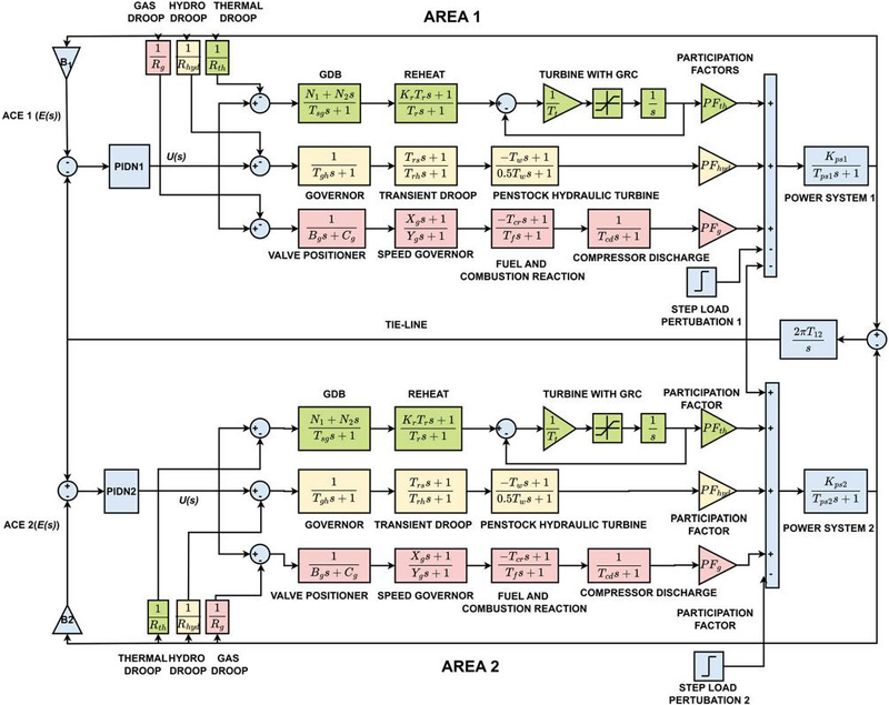
Figure 1 Diverse source interconnected power system transfer function model.
2.2 SSSC Model
SSSC is a Voltage Source Converter (VSC) based FACTS device that is connected to the transmission line in series. Along with the line current, it injects a regulated voltage in quadrature, which alters the line reactance and hence regulates the transmitted power [5]. SSSC doesn’t require inductors or capacitors, thereby reducing the bulkiness of the device. The SSSC model used for this study has been depicted in Figure 2(a). It is represented with a gain of KSSSC and a time constant of TSSSC. Lead and lag compensators are added in cascade with this SSSC with time constants as T1, T2, T3, and T4, where T2 and T4 are usually kept constant to 0.01 seconds [5]. Equation (1) shows how SSSC alters the initial tie line power flow of to the new power flow of .
| (1) |
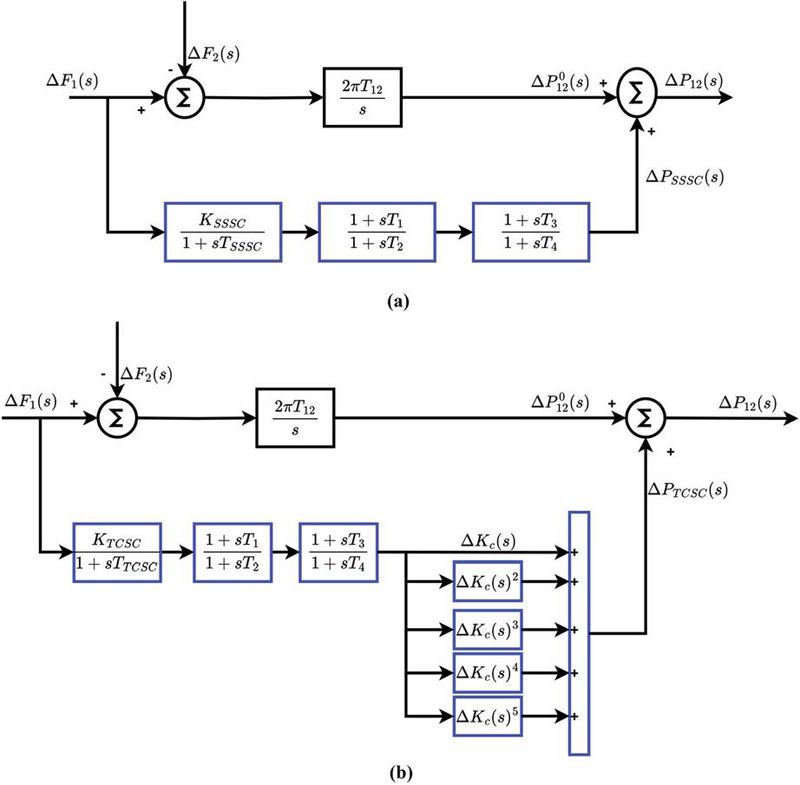
Figure 2 Transfer function model (a) SSSC (b) TCSC.
2.3 TCSC Model
As one of the early FACTS controllers, the TCSC includes a series capacitor bank in parallel with a thyristor-controlled reactor. Control of the thyristor firing angle alters the circuit’s effective reactance, thus regulating power transmission. TCSC offers fast damping of low-frequency oscillations by dynamically adjusting line reactance, thereby improving stability [5]. The transfer function illustration of TCSC is revealed in Figure 2(b). In Equation (2) represents incremental tie-line exchange from area-1 to area-2 without TCSC, is the synchronizing constant, while and are frequency deviances of area-1 and area-2, respectively. The change and control achieved by TCSC in tie line power flow could be expressed using a Taylor series expansion and is shown as in Equation (2) [19]. Here is an input control signal in area 1, while and are the gain and time constant of the TCSC signal conditioning transfer function block. T2 and T4, similar to SSSC, are kept constant at 0.01 seconds while tuning other parameters.
| (2) |
2.4 IPFC Model
IPFC is one of the advanced FACTS devices which employs multiple VSCs connected in series with different transmission lines and shares a common DC link. This helps in coordinated power flow control of multiple lines simultaneously. Due to this feature, IPFC could serve as a supplementary damping controller to dampen frequency oscillations caused by load disturbances. Its model is illustrated in Figure 3(a). In Equation (3) the change in power flow, which could be achieved by IPFC, is represented as , while similar to SSSC and TCSC representation, represents variation in tie line exchange between area-1 and 2 without IPFC, whereas and are frequency change in area-1 and 2, respectively. Here, and are feedback gains, while is the time constant of the IPFC block [5].
| (3) |
2.5 UPFC Model
UPFC is one of the most versatile FACTS devices, which can combine functionalities of both series and shunt compensation. It employs two VSCs, which are connected in series and shunt to the transmission line, and are coupled through a common DC link. The purpose of a shunt converter is to regulate bus voltage and provide reactive support, whereas a series converter helps in regulating the power flow through the line by injecting controllable voltage. UPFC could be used for enhancing tie-line power regulation by controlling voltage, impedance, and phase angle, and thereby offering superior damping of frequency oscillations. For LFC studies, the accurate modelling of UPFC is achieved by the following transfer function representation shown in Equation (4), where represents the time constant of the UPFC block, is the change in frequency in area 1 after a load disturbance, and represents the power flow control which is achieved by UPFC controller [20]. Using this equation, the transfer function illustration of UPFC is shown in Figure 3(b).
| (4) |
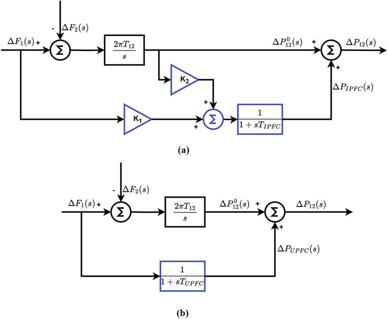
Figure 3 Transfer function model (a) IPFC (b) UPFC.
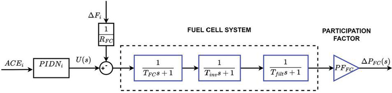
Figure 4 Fuel Cell transfer function model.
2.6 Fuel Cell Model
Hydrogen as an energy source has gained popularity recently due to its efficient and eco-friendly energy generation. In this research, the effect of the addition of FC to the power system in coordination with FACTS devices is explored. Within the FC, hydrogen is fed into the anode such that a catalyst helps to separate hydrogen molecules into protons and electrons. These electrons are channelled through an external circuit to generate an electric current, and protons move through the electrolyte to reach the cathode. Within the cathode, the protons along with electrons and oxygen from atmospheric air combine to give an output of water such that an overall electrochemical reaction is carried out. The transfer function, which represents this process, is expressed as follows and depicted in Figure 4 [18]:
| (5) |
In this equation, 1/R represents the droop characteristics, represent the PIDN controller action, while signifies the participation factor of the FC unit. These values, along with the time constraints of this FC unit, are mentioned in Table A.1 of Appendix [18].
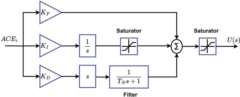
Figure 5 Modified PIDN filter design.
3 Control Strategy
3.1 Modified PIDN Control Design
The controller employed in this research is a modified-PIDN controller, which is designed to effectively mitigate tie-line power and frequency oscillations in an interconnected grid. The controller integrates three distinct control actions of proportional, improved integral and improved derivative action. The proportional part, being the same as conventional PID, provides an immediate corrective effort to the error signal. While integral action is responsible for reducing steady state error, it often winds up during larger disturbances or actuator limits; therefore, an anti-windup mechanism is incorporated using a saturation block, which provides faster and effective action. Further, a low-pass filter is added in addition to the derivative component, which is responsible for improving system dynamics. This filter helps in avoiding amplification of high-frequency noises, ensures practical implementation and enhances robustness to the conventional PID filter. In addition to all these improvements, an output saturation block is also placed after the complete PID action, which ensures practical operational bounds and aligns the dynamics of the modified-PIDN controller with the governor actions of the grid. Figure 5 highlights the control architecture of the modified PIDN controller, as also expressed in Equation (6). The corresponding parameters are listed in Table A.2 of the Appendix. This control structure is deployed in both areas, which are independently tuned using different optimisation algorithms such as GWO, ABC, and DE by reducing a predefined objective function, described in the next subsection.
| (6) |
In this equation, E(s) represents the Area control Error (ACE) of each area of the interconnected grid, which is fed to the modified PIDN controller, while K_pi, K_ii and K_di represent the proportional, integral and derivative gain of the controllers in both areas of the model. Further, T_N represent the time constant of the low-pass filter, and finally U(s) is the control action of this controller.
3.2 Performance Index
The objective function is a crucial component of an effective control scheme. It is formulated to be minimized in order to achieve the desired performance, which in this case involves tweaking the parameters of FACTS and PID controllers. Since the primary objective of LFC studies is to reduce the settling time and minimise the peaks of frequency and tie line oscillations, ITAE is adopted as an objective function. The time multiplication term in ITAE effectively penalizes prolonged variations in system frequency and tie line power, which helps in reducing settling time. In addition, by considering the absolute error in its formulation, ITAE efficiently suppresses peak overshoots and undershoots [10]. This ITAE-based cost index to reduce frequency deviations and tie line power flow changes is stated as follows:
| (7) |
Where is the simulation time, and are the respective frequency variations in areas 1&2, and is the change in tie-line power flow. Minimising this objective function ensures that frequency and tie line power variations are reduced promptly.
3.3 Grey Wolf Optimisation
GWO was presented by Mirjalili in 2014, which is a swarm intelligence-based algorithm. This optimisation works on the hunting behaviour of grey wolves, which prefer to stay in groups of sizes five to twelve individuals. To implement this algorithm, the following steps of social hierarchy, encircling and attacking prey must be followed [8, 13].
1. Social Hierarchy: In the GWO algorithm, wolves are divided into four groups: (leader), (second level), (third level), and (followers). The optimization process is guided by the hunting strategy, where , , and guide the search and follows them. Also, represents the most optimal result, while and represent the second and third finest solutions.
2. Encircling prey: Grey wolves hunt their prey by encircling it. This behaviour could be mathematically represented as follows:
| (8) | |
| (9) |
Where represents the present iteration, and represent the position vector of the prey and wolf. Here and are the coefficient vectors, which are further computed in Equation (10), where and are irregular random ranging [0, 1] and is the decay factor linearly decaying from 2 to 0.
| (10) |
3. Hunting: Since Alpha, Beta and Delta are the best ways to reach the prey, the path between Omega wolves and these three optimum wolves is computed, and Omega’s position is changed as follows:
| (11) | |
| (12) | |
| (13) | |
| (14) | |
| (15) | |
| (16) | |
| (17) |
Here , , represent the positions of three optimum wolves. The vectors , , denote coefficient vectors and , , are parameters that control the balance between exploration and exploitation associated with these three leaders. Terms , , represent the calculated distance between the current wolf and each of the three leaders. Finally, , , correspond to the estimated new positions of the wolf with respect to the alpha, beta, and delta wolves. Some of the constraints used in the GWO for this research are listed in Table A.2 in the appendix. GWO could be better understood from the algorithm shown in Figure 6(a).
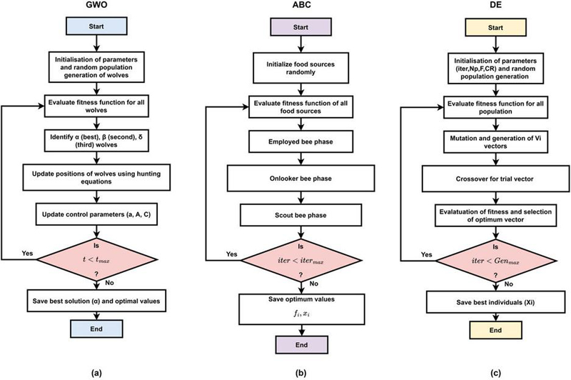
Figure 6 Flowcharts of optimisation algorithms (a) GWO (b) ABC (c) DE.
3.4 Artificial Bee Colony
The ABC algorithm is a population-based algorithm which works on the foraging behaviour of honeybees. It has been widely used in engineering optimisation due to its simplicity, robustness and fast convergence characteristics. In the LFC problem, the decision vector contains the controller parameters to be optimised, which are parameters of FACTS devices and the controller. The ABC algorithm iteratively improves a population of nominee solutions (food sources) using three types of agents: Employed Bees (EB), Onlooker Bees (OB), and Scout Bees (SB). EB explores surrounding of their assigned food sources, OB probabilistically select promising sources based on nectar quality (fitness), and SB perform random exploration to replace abandoned sources. This process of finding an optimal solution for solving this problem using ABC optimisation could be divided into the following phases [32]:
1. Initialisation: Firstly, each decision variable is initialised uniformly within its bounds as follows:
| (18) |
In this equation, represents the current food source and is varied from in this expression, while represents the dimensionality of each solution vector and is varied from . After initialisation of the decision variable, the cost function (ITAE) corresponding to randomly generated variables is mapped such that the lower cost function corresponds to a higher fitness value using the following mapping technique:
| (19) |
2. EB phase: In this phase, each EB explore other food sources in the surroundings of the current assigned food source (). Hence, a new contender is generated by perturbing a randomly selected neighbour as follows:
| (20) |
If the new candidate result goes out of its bounds [], it is clipped to its bounds. Further, greedy selection is applied to this process, and if achieves an improved fitness value than the current solution , then it is selected. Since the food sources drain after some iterations, a limit is set on each trial represented as . When better is found with better fitness value, the counter is reset; else the counter is increased.
3. OB phase: In this phase, each OB selects a food source () with the probability and around this selected food source, a neighbour using Equation (20) is evaluated, and greedy selection is performed similarly as in the EB phase. The counter is also updated as in the EB phase. The selection probability for each food source is calculated based on fitness values according to normalised roulette-wheel style probability as depicted in the following equation:
| (21) |
4. SB phase: In this phase, exploited food sources are abandoned, and new food sources are randomly generated using equation 18. This is done when the counter reaches its maximum value, which helps in avoiding local minima solutions. Once a new food source is selected, this counter is reset. These steps of EB, OB, and SB are followed until all the iterations are performed. Some of the constraints used in the ABC algorithm of this research are listed in Table A.2 in the appendix, while Figure 6(b) shows how the ABC algorithm works.
3.5 Differential Evolution
DE is a robust, population-based algorithm which is explicitly efficient for solving nonlinear and non-differentiable complications such as LFC. It works by iteratively improving possible population contender solutions using mutation, crossover, and selection operators. The algorithm is simple in structure yet powerful in exploring and exploiting the solution space. Some of the factors employed in the DE algorithm of this research are listed in Table A.2 in the appendix. The following steps explain the working of DE, and Figure 6(c) explains the algorithm of DE pictorially [33]:
1. Initialisation: Initially, a population of NP individuals which represent a potential solution is generated randomly while maintaining the parameters within their bounds:
| (22) |
Here, is the count for the population of individuals, is the dimension.
2. Mutation: For the randomly generated target vector in generation , a mutant vector is generated as follows:
| (23) |
Here are distinct indices other than , and is the scaling factor.
3. Crossover: Crossover of the generated generation is performed between the target vector ( and the mutant vector ( so that the diversity could be increased, and the trial vector is formed as follows:
| (24) |
Where denotes the crossover probability within the interval (0,1), is a random variable uniformly distributed in [0, 1], and is a arbitrarily chosen index ensuring at least one parameter comes from the mutant.
4. Selection: The trial vector is then evaluated, and the vector that yields the least cost function is selected. This procedure continues until the algorithm reaches the specified generational limit. The trial vector evaluation is as follows:
| (25) |
4 Results and Discussion
This research analyses the dynamic performance of a realistic diverse-source interconnected grid under four operating case scenarios. In addition, different control strategies are examined under an enhanced PIDN controller design, which is optimally tuned by three optimisation algorithms, namely GWO, ABC and DE, in coordination with four FACTS devices, namely SSSC, TCSC, IPFC, and UPFC, are investigated. To achieve this, a comparative performance evaluation of the three algorithms is first presented. Subsequently, variable load perturbation scenarios are investigated in Case Scenarios 1, 2, and 3. Finally, the influence of incorporating the FC unit with the conventional grid, in coordination with FACTS controllers, is assessed in Case Scenario 4.
4.1 Comparative performance of GWO, ABC and DE
This research initially investigates the most effective optimisation technique for tuning the PIDN controller to reduce frequency oscillations in a two-area interconnected grid. For this purpose, the GWO, ABC, and DE algorithms are employed to optimise the controller parameters by minimising the selected performance index, ITAE. A step load perturbation (SLP) of 1% is applied in Area-1 of the designed framework, resulting in variations in the frequencies and tie-line power exchange. During simulation, these algorithms determine the optimal PIDN controller parameters by minimising the ITAE over the desired number of iterations, as listed in Table 1. When implemented in the controller, these optimal values effectively reduce frequency and tie-line power variations. Table 2 presents key performance indicators, including ITAE, settling time, peak undershoot, and peak overshoot, obtained by each algorithm. It is evident from this table that the GWO-based approach achieves least ITAE value of 0.002809, confirming its superior error-minimisation capability. A smaller ITAE corresponds to improved damping of oscillations and faster convergence of errors, both of which are critical for maintaining LFC stability.
Table 1 Optimised controller parameters from GWO, ABC and DE
| Controllable Parameters | PIDN-GWO | PIDN-ABC | PIDN-DE |
| KP1 | 1.1769 | 1.1446 | 1.2094 |
| KI1 | 2 | 2 | 1.999 |
| KD1 | 1 | 1 | 1 |
| KP2 | 1.1358 | 1.0764 | 1.0902 |
| KI2 | 0.2388 | 0.3827 | 0.2633 |
| KD2 | 1 | 1 | 1 |
Table 2 Comparative control performance of GWO, ABC, and DE
| Settling | Undershoot | Overshoot | |||
| Algorithm | Deviation | ITAE | Time (s) | (10-4) | (10-4) |
| GWO | F1 | 0.002809 | 10.7257 | 2.8157 | 0.754 |
| F2 | 12.0363 | 2.0697 | 0.633 | ||
| Ptie | 11.8405 | 0.4503 | 0.0677 | ||
| ABC | F1 | 0.002825 | 10.5696 | 2.8162 | 0.791 |
| F2 | 9.8053 | 2.077 | 0.653 | ||
| Ptie | 16.3142 | 0.4514 | 0.0627 | ||
| DE | F1 | 0.002811 | 10.7404 | 2.8152 | 0.755 |
| F2 | 12.0181 | 2.0629 | 0.635 | ||
| Ptie | 14.7228 | 0.4495 | 0.0655 |
In terms of Settling Time, the ABC algorithm achieves the fastest response in the case of deviations in frequency in Area 2 and settles the variation in 9.80 seconds, while GWO settles the variations in Area 1 and 2 in 10.73 seconds and 12.04 seconds, respectively. However, this advantage is offset by its poor tie-line dynamics, where ABC requires 16.31 seconds compared to GWO, which requires 11.84 seconds to settle the deviations, indicating weaker inter-area coordination. DE delivers an ITAE similar to GWO (0.002811) but takes longer to stabilise tie-line fluctuations (14.72 s), making it less effective for enhancing inter-area stability. In terms of Settling Min and Settling Max, all three algorithms achieve very close results; however, GWO keeps deviations during transients small, limiting undershoot and ensuring bounded overshoot consistently. Furthermore, Figure 7 presents the convergence characteristics of all three algorithms during the PIDN parameter optimisation process to provide better insights into their search efficiency and stability. This also solidifies that GWO achieves the best trade-off between speed, accuracy, and stability. It reduces ITAE more effectively while maintaining moderate settling times across all responses. Hence, GWO is chosen as the optimisation algorithm for further investigation of the coordinated damping control strategy of PIDN and FACTS devices and also to study the consequences of the FC unit on frequency stability.
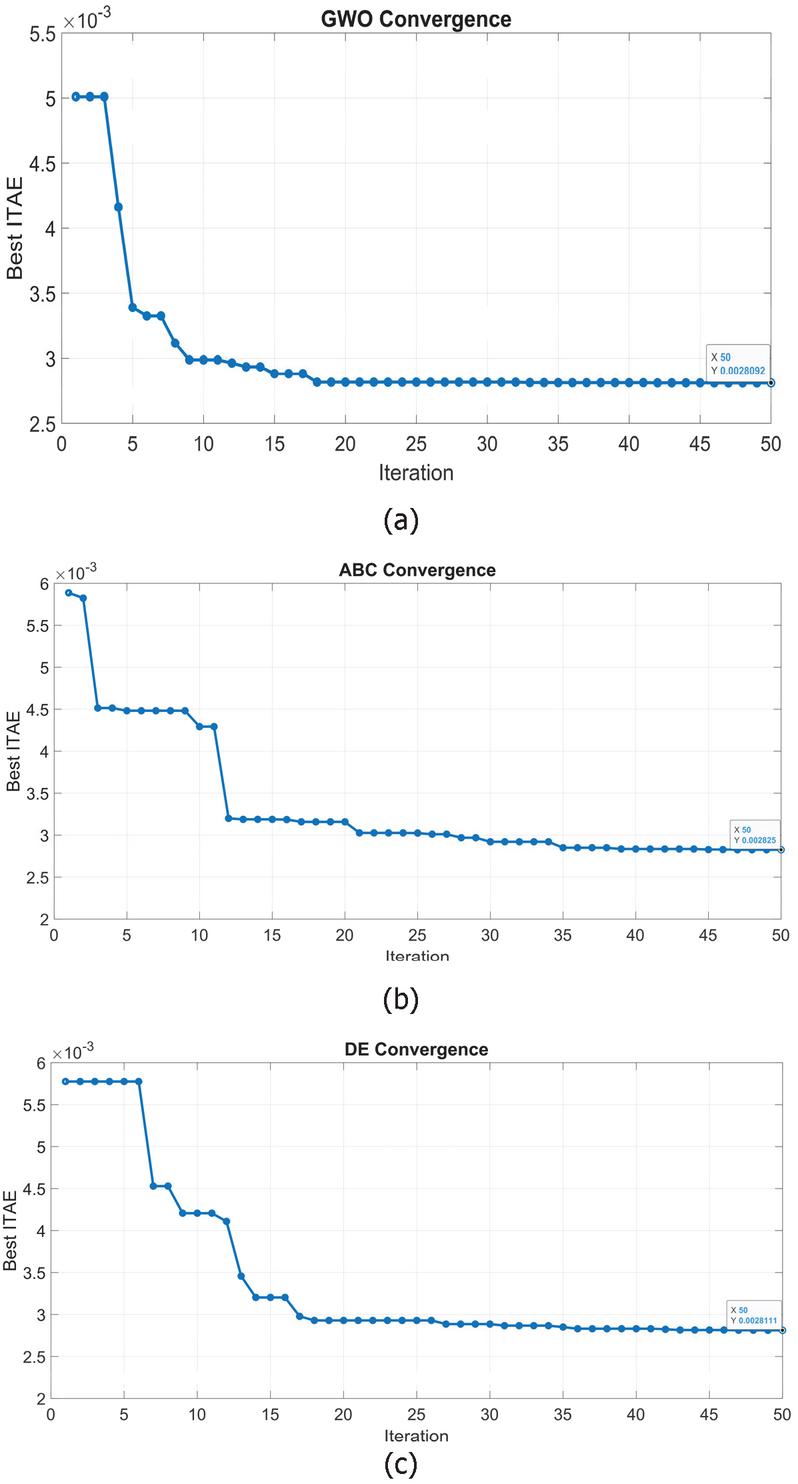
Figure 7 Convergence plot (a) GWO (b) ABC (c) DE.
Table 3 Tuned controllable parameters using GWO under various scenarios
| Control | Controllable | ||||
| Strategy | Parameters | Scenario-1 | Scenario-2 | Scenario-3 | Scenario-4 |
| PIDN-GWO | KP1 | 1.1769 | 1.1291 | 0.4281 | 1.9795 |
| KI1 | 2 | 0.2769 | 1.3747 | 2 | |
| KD1 | 1 | 1 | 1 | 1 | |
| KP2 | 1.1358 | 1.1725 | 1.0885 | 1.8372 | |
| KI2 | 0.2388 | 2 | 1.9083 | 0.4286 | |
| KD2 | 1 | 1 | 1 | 1 | |
| PIDN-GWO-SSSC | KP1 | 2 | 1.3024 | 0.104 | 2 |
| KI1 | 2 | 1.6013 | 1.082 | 2 | |
| KD1 | 0.819 | 1 | 0.0057 | 0.4404 | |
| KP2 | 1.7923 | 2 | 2 | 1.5701 | |
| KI2 | 0.3474 | 2 | 2 | 0.3674 | |
| KD2 | 0.999 | 1 | 1 | 1 | |
| KSSSC | 0.1418 | 0.4649 | 2 | 0.2584 | |
| TSSSC | 0.6183 | 1 | 0.4865 | 0.9458 | |
| T1 | 0.1476 | 0.2793 | 0.0772 | 0.1671 | |
| T3 | 0.5551 | 0.021 | 0.0572 | 0.5228 | |
| PIDN-GWO-TCSC | KP1 | 2 | 1.3127 | 0.4733 | 2 |
| KI1 | 2 | 1.5158 | 1.1895 | 2 | |
| KD1 | 0.9919 | 1 | 0.191 | 0.478 | |
| KP2 | 1.9547 | 2 | 1.9956 | 1.885 | |
| KI2 | 0.3577 | 2 | 2 | 0.3801 | |
| KD2 | 1 | 1 | 0.9963 | 1 | |
| KTCSC | 0.1309 | 0.5326 | 1.9984 | 0.2156 | |
| TTCSC | 0.8832 | 0.9994 | 0.9305 | 0.8456 | |
| T1 | 0.5487 | 0.1524 | 0.2741 | 0.0208 | |
| T3 | 0.3364 | 0.127 | 0.0637 | 0.8904 | |
| PIDN-GWO-IPFC | KP1 | 2 | 0.6203 | 0.4475 | 2 |
| KI1 | 2 | 0.577 | 1.2959 | 2 | |
| KD1 | 1 | 0.9604 | 0.2047 | 0.5866 | |
| KP2 | 2 | 2 | 2 | 2 | |
| KI2 | 0.4465 | 2 | 2 | 0.4182 | |
| KD2 | 1 | 0.7676 | 1 | 1 | |
| TIPFC | 0.0214 | 0.0685 | 0.0894 | 0.0151 | |
| K1 | 0.346 | 0.2625 | 1.509 | 0.3948 | |
| K2 | 0.311 | 1.5331 | 1.8268 | 1.1927 | |
| PIDN-GWO-UPFC | KP1 | 2 | 1.0164 | 0.3523 | 2 |
| KI1 | 2 | 2 | 1.2453 | 2 | |
| KD1 | 0.4259 | 0.6955 | 0.1305 | 0.141 | |
| KP2 | 2 | 2 | 2 | 2 | |
| KI2 | 0.9046 | 2 | 2 | 2 | |
| KD2 | 1 | 1 | 1 | 1 | |
| TUPFC | 0.0718 | 0.0214 | 0.1433 | 0.085 |
4.2 Scenario-1
In this scenario, a 1% SLP is applied in area 1 of the interconnected grid. This causes an increase in power demand in area 1, leading to a temporary fall in frequency in both areas and producing oscillations in frequency and tie-line. GWO was used for the tuning of several controllable parameters for different control strategies, and the obtained values of these parameters are mentioned in Table 3. It is evident from Table 4 that when different FACTS devices were integrated with the PIDN-GWO control strategy, a substantial reduction in the cost function ITAE is achieved. For instance, PIDN-GWO-TCSC and PIDN-GWO-IPFC strategies obtained ITAE of 0.002302 and 0.002320, respectively, compared to the base case of PIDN-GWO, where the cost function is 0.002809. Transient analysis from Table 5 indicates that the TCSC and SSSC configurations offered faster rise times in case of variations in frequencies of both areas and significantly reduced peak overshoot compared to the base PIDN–GWO controller. In addition to this, the superior performance of IPFC is evident in the case of settling oscillation faster in tie-line power flows by settling it in 8.6 seconds. Compared to all FACTS devices, UPFC exhibited the slowest settling in the case of frequency fluctuation in area 1 in 12.6 seconds. Figure 8 showcases the plot of the variations in frequencies and tie-line power flow amongst different control strategies.
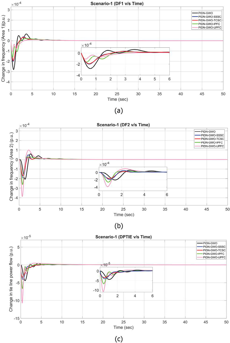
Figure 8 Scenario-1 (a) Variations in frequency (Area-1) (b) Variations in frequency (Area-2) (c) Variation in tie line power flow.
Table 4 ITAE in different scenarios using various control strategies
| ITAE | ||||
| Control Strategy | Scenario-1 | Scenario-2 | Scenario-3 | Scenario-4 |
| PIDN-GWO | 0.002809 | 0.00281 | 0.002955 | 0.002044 |
| PIDN-GWO-SSSC | 0.00232 | 0.002438 | 0.001434 | 0.001867 |
| PIDN-GWO-TCSC | 0.002302 | 0.002442 | 0.001458 | 0.001883 |
| PIDN-GWO-IPFC | 0.002337 | 0.002414 | 0.001303 | 0.001886 |
| PIDN-GWO-UPFC | 0.002483 | 0.002636 | 0.001611 | 0.001978 |
Table 5 Control performance of different control strategies
| Scenario-1 | Scenario-2 | Scenario-3 | Scenario-4 | ||||||||||
| Control Strategy | Control Parameter | F1 | F2 | PTIE | F1 | F2 | PTIE | F1 | F2 | PTIE | F1 | F2 | PTIE |
| PIDN-ALG | Rise Time (s) | 0.00016 | 0.0002 | 0.0017 | 0.0002 | 0.0001 | 0.0016 | 0.00008 | 0.00003 | 0.0078 | 0.0003 | 0.0014 | 0.0296 |
| Peak Undershoot (10-4)(p.u.) | 2.8104 | 2.0643 | 0.4431 | 0.5945 | 0.7256 | 0.4499 | 1.5624 | 2.6209 | 0.0604 | 2.1102 | 1.2351 | 0.3099 | |
| Peak Overshoot (10-4)(p.u.) | 0.6553 | 0.5905 | 0.045 | 2.0741 | 2.8152 | 0.0536 | 1.1239 | 1.322 | 0.67 | 0.2612 | 0.0884 | 0.0103 | |
| Settling Time (s) | 9.3141 | 10.6536 | 12.7339 | 10.6288 | 9.2379 | 13.1519 | 10.7322 | 7.6524 | 16.9641 | 9.7172 | 12.4116 | 17.5905 | |
| PIDN-ALG-SSSC | Rise Time (s) | 0.001 | 0.00029 | 0.0173 | 0.0019 | 0.0003 | 0.0213 | 0.00005 | 0.000005 | 0.0112 | 0.0031 | 0.0005 | 0.0441 |
| Peak Undershoot (10-4)(p.u.) | 1.998 | 1.9346 | 0.4099 | 0.0999 | 0.6666 | 0.2636 | 0.074 | 1.6792 | 0.0561 | 1.6046 | 1.6041 | 0.3991 | |
| Peak Overshoot (10-4)(p.u.) | 0.3663 | 0.4908 | 0.0118 | 1.2163 | 2.8493 | 0.0211 | 0.4256 | 0.4661 | 0.6656 | 0.0889 | 0.2499 | 0.0087 | |
| Settling Time (s) | 10.9754 | 10.7597 | 15.4122 | 12.9059 | 8.1917 | 20.2132 | 12.7667 | 5.0496 | 16.6375 | 11.3733 | 10.3887 | 11.4311 | |
| PIDN-ALG-TCSC | Rise Time (s) | 0.00096 | 0.00048 | 0.0238 | 0.0027 | 0.0002 | 0.022 | 0.00007 | 0.000002 | 0.0145 | 0.0016 | 0.0003 | 0.0466 |
| Peak Undershoot (10-4)(p.u.) | 1.9317 | 1.6894 | 0.345 | 0.071 | 0.6551 | 0.2508 | 0.1282 | 1.631 | 0.0455 | 1.5937 | 1.7763 | 0.4544 | |
| Peak Overshoot (10-4)(p.u.) | 0.3307 | 0.2692 | 0.013 | 1.1622 | 2.863 | 0.0201 | 0.4089 | 0.32115 | 0.5624 | 0.1109 | 0.2893 | 0.0091 | |
| Settling Time (s) | 11.0603 | 11.3853 | 17.4039 | 13.0694 | 8.3202 | 20.7114 | 11.7534 | 7.0885 | 17.6676 | 11.3168 | 10.0283 | 4.1224 | |
| PIDN-ALG-IPFC | Rise Time (s) | 0.0019 | 0.0003 | 0.0051 | 0.0012 | 0.0005 | 0.002 | 0.00006 | 0.00019 | 0.0093 | 0.0033 | 0.0007 | 0.0313 |
| Peak Undershoot (10-4)(p.u.) | 1.5945 | 2.6155 | 0.6647 | 0.285 | 0.3724 | 0.5021 | 0.2054 | 1.4985 | 0.0584 | 1.2062 | 2.0959 | 0.5951 | |
| Peak Overshoot (10-4)(p.u.) | 0.2076 | 0.313 | 0.014 | 2.0803 | 2.6234 | 0.0188 | 0.3818 | 0.31682 | 0.7324 | 0.1026 | 0.164 | 0.0108 | |
| Settling Time (s) | 11.5781 | 8.5945 | 8.6494 | 9.6822 | 8.9033 | 18.2248 | 7.6956 | 4.7239 | 16.1563 | 12.366 | 9.0825 | 3.1467 | |
| PIDN-ALG-UPFC | Rise Time (s) | 0.0062 | 0.00021 | 0.003 | 0.1089 | 0.0001 | 0.0243 | 0.00006 | 0.00004 | 0.0157 | 0.0342 | 0.0001 | 0.0112 |
| Peak Undershoot (10-4)(p.u.) | 1.0949 | 3.8693 | 1.0725 | 0.0279 | 1.0439 | 0.1133 | 0.0859 | 1.8385 | 0.0405 | 0.9989 | 3.237 | 0.9627 | |
| Peak Overshoot (10-4)(p.u.) | 0.09 | 1.001 | 0.049 | 0.5742 | 2.9793 | 0.0174 | 0.5495 | 0.2766 | 0.6771 | 0.0324 | 0.587 | 0.031 | |
| Settling Time (s) | 12.5553 | 6.3695 | 8.5741 | 20.1889 | 8.6312 | 26.1035 | 9.5258 | 7.5866 | 17.3057 | 12.4936 | 3.6427 | 9.613 | |
4.3 Scenario-2
In this scenario, a 1% SLP is applied in area 2 of the interconnected grid, which indicates a fall in power demand in area 2. This change in power demand produces oscillations in frequencies and tie-line due to the interconnected grid. Similar to Scenario-1, GWO was used for the tuning of several controllable parameters, and the obtained values of these parameters are stated in Table 3. The ITAE values mentioned in Table 4 show that the IPFC-based control strategy achieves the least value of 0.002414, outperforming SSSC and TCSC with ITAE values of 0.002438 and 0.002442, respectively. From the transient perspective, the PIDN-GWO-SSSC approach provided the most balanced response with settling fluctuations in frequency in this area in 8.2 seconds. Similar to Scenario-1, UPFC again exhibited very long settling times, particularly in tie-line flows, highlighting its inefficiency compared to other FACTS-based approaches. The base PIDN-GWO strategy also provided moderate damping but produced higher overshoots in the frequency variations of area 2. Table 5 explicitly explains the effectiveness of these control strategies based on their transient performance. Figure 9 showcases the plot of the variation in frequencies and tie-line power flow amongst different control strategies.
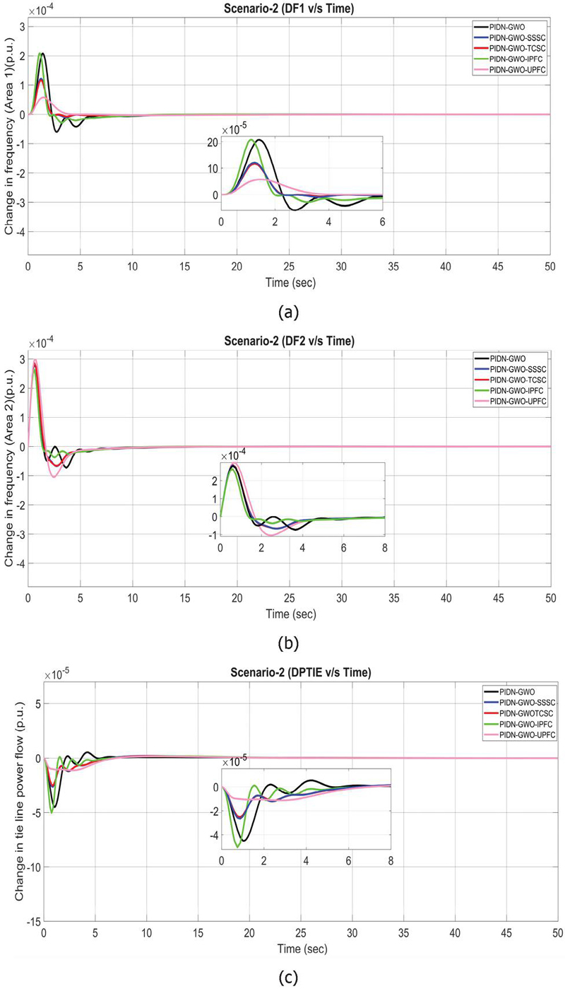
Figure 9 Scenario-2 (a) Variations in frequency (Area-1) (b) Variations in frequency (Area-2) (c) Variation in tie line power flow.
4.4 Scenario-3
This scenario imposes simultaneous disturbances in both areas with 0.5% SLP in Area 1 and +1% SLP in Area 2. The ITAE values from Table 4 clearly show that the PIDN-GWO-IPFC strategy offers the best performance by minimising the cost function to 0.001303 compared to its competitors, TCSC and SSSC, which achieve ITAE of 0.001458 and 0.001434, respectively. Control performance analysis from Table 5 indicates that IPFC integration drastically improves the rise time of F2 to 0.19 milliseconds and reduces the peak undershoot of to . Furthermore, IPFC and SSSC both limited overshoot to p.u., considerably lower than the base PIDN–GWO case. Settling times for were also improved, with the PIDN-GWO-IPFC strategy, which was reduced to 16.1 seconds compared to 17 seconds for the base controller. These results confirm that IPFC is highly effective in scenarios involving multi-area simultaneous disturbances. These control performances could be better visualised from Figure 10.
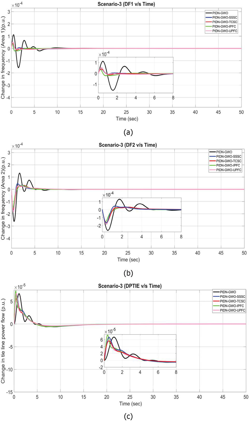
Figure 10 Scenario-3 (a) Variations in frequency (Area-1) (b) Variations in frequency (Area-2) (c) Variation in tie line power flow.
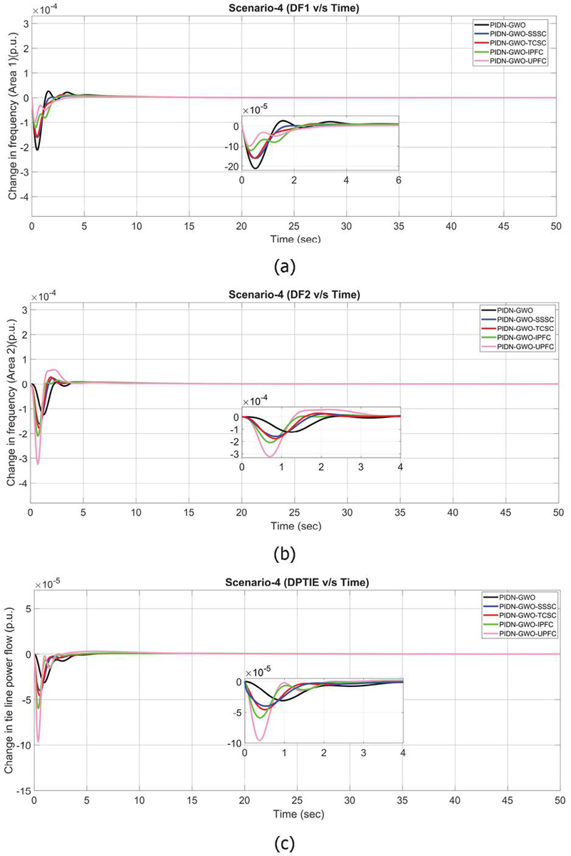
Figure 11 Scenario-4 (a) Variations in frequency (Area-1) (b) Variations in frequency (Area-2) (c) Variation in tie line power flow.
4.5 Scenario-4
This scenario investigates the effect of the inclusion of FC with the conventional grid in coordination with the FACTS devices. In this case, FC is designed to contribute to 10% of the load demands, and hence, a participation factor of 0.1 is kept for this FC unit. Since the inclusion of FC increases power sources, the participation factors of each reheat-thermal, gas, and hydro unit are reduced to 90% of their initial value, maintaining the overall rated capacity of the interconnected grid identical. After integration of the FC unit, an SLP of 1% is induced in Area 1 to produce power oscillations. Further, similar control strategies, namely PIDN-GWO, PIDN-GWO-SSSC, PIDN-GWO-TCSC, PIDN-GWO-IPFC and PIDN-GWO-UPFC, are analysed for this modified power system.
From Table 4, it is evident that this modified power system with the FC unit performs superiorly compared to the first case scenario with similar SLP in all the control strategies. Even the base control strategy of PIDN-GWO in this scenario outperforms the best control strategy in scenario 1, with an ITAE value of 0.002044 compared to 0.002302 in that scenario for PIDN-GWO-TCSC. Moving forward, FACTS devices in this scenario produced very similar ITAE values for SSSC, TCSC and IPFC-based approach. The control performance mentioned in Table 5 highlights that the IPFC-based technique achieves the shortest settling time for of 3.14 seconds, followed by the TCSC-based approach with 4.12 seconds. This demonstrates their superior coordination with the FC in dampening tie-line oscillations. The SSSC, while yielding favourable ITAE, showed comparatively larger settling times. The UPFC again recorded the poorest dynamic responses, with higher peak undershoots and longer settling times. Summing up, Scenario 4 highlights that the FC integration enhances the damping capability of the grid, and its further integration with optimally tuned FACTS devices, such as IPFC and SSSC, could further improve the frequency stability of the power system.
5 Conclusion
This work presented a comprehensive investigation of frequency stability enhancement and tie-line power regulation in a nonlinear two-area interconnected power system comprising reheat-thermal, gas and hydro units. A modified PIDN controller with derivative filtering and anti-windup protection was designed, and its parameters, along with those of FACTS devices, were optimally tuned using three population-based metaheuristic algorithms, namely GWO, ABC, and DE. Furthermore, the impact of integrating an FC unit as a clean energy source was analysed to assess its contribution to frequency regulation. The obtained results demonstrate that GWO consistently outperforms ABC and DE by achieving ITAE values, as low as 0.002044, under FC-integrated multi-area disturbances, yielding superior transient response with reduced overshoot and undershoot confined within p.u. limits, along with faster settling times across all studied scenarios. Further, inclusion of the FC unit strengthened system resilience by reducing ITAE by approximately 25–30% compared to the corresponding cases without FC integration, highlighting the role of cleaner energy sources as dynamic frequency support. Among the FACTS devices investigated, IPFC consistently delivered the best overall performance by reducing ITAE upto 55% in Scenario-3 compared to the base PIDN–GWO case. Summating up, this study clearly establishes that the coordinated deployment of an optimally tuned PIDN controller, FC-based generation, and FACTS devices can substantially enhance frequency stability in interconnected power systems. However, future research can explore the proposed methodology in larger multi-area systems with high renewable penetration, exploring hybrid energy storage systems for enhanced inertia support, and leveraging advanced intelligent optimisation methods, including reinforcement learning and digital twin frameworks, for real-time adaptive frequency regulation.
Appendix
Table A.1 : Fixed parameters used for power system modelling
| System | Specifications |
| Thermal Powerplant | N, N, T s, KrT s, T s, T s, PF |
| Hydro Powerplant | T s, T s, T s, T s, PF |
| Gas Powerplant | C, X, B, T s, T s, T s, T s, PF |
| Power system parameters | Hz/p.u, p.u.MW/Hz, T s, K, T s |
| Fuel Cell | T s, T s, T s |
Table A.2 : Fixed parameters of control strategy
| Controller & Algorithms | Specifications |
| PIDN | Anti saturation limit 0.5 & 1, T |
| GWO | Iter(t) 50, Search_agents 20 |
| ABC | Iter 50, Colony_size 20, Food_sources(SN) 10 |
| DE | Iter(Gen) 50, N, F 0.8, CR 0.9 |
References
[1] M. Ranjan and R. Shankar, “A literature survey on load frequency control considering renewable energy integration in power system: Recent trends and future prospects,” Journal of Energy Storage, vol. 45, p. 103717, Jan. 2022, doi:10.1016/j.est.2021.103717.
[2] R. Asghar, F. Riganti Fulginei, H. Wadood, and S. Saeed, “A Review of Load Frequency Control Schemes Deployed for Wind-Integrated Power Systems,” Sustainability, vol. 15, no. 10, p. 8380, May 2023, doi:10.3390/su15108380.
[3] K. Peddakapu, M. R. Mohamed, P. Srinivasarao, Y. Arya, P. K. Leung, and D. J. K. Kishore, “A state-of-the-art review on modern and future developments of AGC/LFC of conventional and renewable energy-based power systems,” Renewable Energy Focus, vol. 43, pp. 146–171, Dec. 2022, doi:10.1016/j.ref.2022.09.006.
[4] M. Wadi, A. Shobole, W. Elmasry, and I. Kucuk, “Load frequency control in smart grids: A review of recent developments,” Renewable and Sustainable Energy Reviews, vol. 189, p. 114013, Jan. 2024, doi:10.1016/j.rser.2023.114013.
[5] I. A. Khan, H. Mokhlis, N. N. Mansor, H. A. Illias, L. Jamilatul Awalin, and L. Wang, “New trends and future directions in load frequency control and flexible power system: A comprehensive review,” Alexandria Engineering Journal, vol. 71, pp. 263–308, May 2023, doi:10.1016/j.aej.2023.03.040.
[6] B. Singh, A. Slowik, and S. K. Bishnoi, “Review on Soft Computing-Based Controllers for Frequency Regulation of Diverse Traditional, Hybrid, and Future Power Systems,” Energies, vol. 16, no. 4, p. 1917, Feb. 2023, doi:10.3390/en16041917.
[7] A. Latif, S. M. S. Hussain, D. C. Das, and T. S. Ustun, “State-of-the-art of controllers and soft computing techniques for regulated load frequency management of single/multi-area traditional and renewable energy based power systems,” Applied Energy, vol. 266, p. 114858, May 2020, doi:10.1016/j.apenergy.2020.114858.
[8] X.-C. Shangguan, S. Shi, Y. He, and C.-K. Zhang, “Optimal Digital Load Frequency Control of Smart Grid Considering Sampling and Time Delay Based on Warm-Up Gray Wolf Algorithm,” IEEE Trans. Ind. Inf., vol. 21, no. 2, pp. 1773–1782, Feb. 2025, doi:10.1109/TII.2024.3485821.
[9] H. Luo and Z. Hu, “Stability Analysis of Sampled-Data Load Frequency Control Systems With Multiple Delays,” IEEE Trans. Contr. Syst. Technol., vol. 30, no. 1, pp. 434–442, Jan. 2022, doi:10.1109/TCST.2021.3061556.
[10] N. K. Gupta, M. K. Kar, and A. K. Singh, “Design of a 2-DOF-PID controller using an improved sine–cosine algorithm for load frequency control of a three-area system with nonlinearities,” Prot Control Mod Power Syst, vol. 7, no. 1, p. 33, Dec. 2022, doi:10.1186/s41601-022-00255-w.
[11] T. Ali et al., “Terminal Voltage and Load Frequency Control in a Real Four-Area Multi-Source Interconnected Power System With Nonlinearities via OOBO Algorithm,” IEEE Access, vol. 12, pp. 123782–123803, 2024, doi:10.1109/ACCESS.2024.3453755.
[12] B. A. Fadheel et al., “A Hybrid Sparrow Search Optimized Fractional Virtual Inertia Control for Frequency Regulation of Multi-Microgrid System,” IEEE Access, vol. 12, pp. 45879–45903, 2024, doi:10.1109/ACCESS.2024.3376468.
[13] S. A. Zaid et al., “A New Intelligent Fractional-Order Load Frequency Control for Interconnected Modern Power Systems with Virtual Inertia Control,” Fractal Fract, vol. 7, no. 1, p. 62, Jan. 2023, doi:10.3390/fractalfract7010062.
[14] H. H. Alhelou, N. Nagpal, N. Kassarwani, and P. Siano, “Decentralized Optimized Integral Sliding Mode-Based Load Frequency Control for Interconnected Multi-Area Power Systems,” IEEE Access, vol. 11, pp. 32296–32307, 2023, doi:10.1109/ACCESS.2023.3262790.
[15] A. Kumar et al., “Load Frequency Control of Distributed Generators Assisted Hybrid Power System Using QOHSA Tuned Model Predictive Control,” IEEE Access, vol. 10, pp. 109311–109325, 2022, doi:10.1109/ACCESS.2022.3214315.
[16] M. Bhukya, S. K. Injeti, R. P. Ogirala, and S. Kotte, “Real-Time Simulation and Validation of Interconnected Microgrid Load Frequency Control With Uncertainties Using PDN-Iλ Dμ Controller Based on Improved Smell Agent Optimization,” IEEE Trans. Ind. Inf., vol. 20, no. 5, pp. 7238–7248, May 2024, doi:10.1109/TII.2024.3353825.
[17] I. A. Khan et al., “Load Frequency Control Using Golden Eagle Optimization for Multi-Area Power System Connected Through AC/HVDC Transmission and Supported With Hybrid Energy Storage Devices,” IEEE Access, vol. 11, pp. 44672–44695, 2023, doi:10.1109/ACCESS.2023.3272836.
[18] I. Kaya, Y. Güler, and M. Nalbantoğlu, “Direct Synthesis-based optimal PIDD2 controller design for enhanced load frequency control in microgrid systems with fuel cells and diesel generators,” Int. J. Hydrogen Energy, vol. 147, p. 149981, 2025, doi:10.1016/j.ijhydene.2025.06.171.
[19] Vigya, C. K. Shiva, B. Vedik, and V. Mukherjee, “Comparative analysis of PID and fractional order PID controllers in automatic generation control process with coordinated control of TCSC,” Energy Syst, vol. 14, no. 1, pp. 133–170, Feb. 2023, doi:10.1007/s12667-021-00457-5.
[20] S. B. Masikana, G. Sharma, S. Sharma, and E. Çelik, “Frequency regulation in solar PV-powered thermal power system using FPA-PID controller through UPFC and RFB,” Electr Eng, May 2024, doi:10.1007/s00202-024-02417-5.
[21] A. T. Salawudeen, M. Moritz, I. Jahn, O. Johnson, and A. Monti, “Enhanced Chameleon Swarm Algorithms for Nested Identical Control of Load Frequency in Autonomous Microgrid,” IEEE Access, vol. 12, pp. 42544–42571, 2024, doi:10.1109/ACCESS.2024.3379296.
[22] A. H. Yakout, H. Kotb, H. M. Hasanien, and K. M. Aboras, “Optimal Fuzzy PIDF Load Frequency Controller for Hybrid Microgrid System Using Marine Predator Algorithm,” IEEE Access, vol. 9, pp. 54220–54232, 2021, doi:10.1109/ACCESS.2021.3070076.
[23] A. Daraz, S. A. Malik, A. T. Azar, S. Aslam, T. Alkhalifah, and F. Alturise, “Optimized Fractional Order Integral-Tilt Derivative Controller for Frequency Regulation of Interconnected Diverse Renewable Energy Resources,” IEEE Access, vol. 10, pp. 43514–43527, 2022, doi:10.1109/ACCESS.2022.3167811.
[24] G. Dei et al., “Improved Squirrel Search Algorithm Driven Cascaded 2DOF-PID-FOI Controller for Load Frequency Control of Renewable Energy Based Hybrid Power System,” IEEE Access, vol. 10, pp. 46372–46391, 2022, doi:10.1109/ACCESS.2022.3169749.
[25] E. Sahin, “Design of an Optimized Fractional High Order Differential Feedback Controller for Load Frequency Control of a Multi-Area Multi-Source Power System With Nonlinearity,” IEEE Access, vol. 8, pp. 12327–12342, 2020, doi:10.1109/ACCESS.2020.2966261.
[26] V. V. Huynh, P. T. Tran, C. S. T. Dong, B. D. Hoang, and O. Kaynak, “Sliding Surface Design for Sliding Mode Load Frequency Control of Multiarea Multisource Power System,” IEEE Trans. Ind. Inf., vol. 20, no. 5, pp. 7797–7809, May 2024, doi:10.1109/TII.2024.3359445.
[27] A.-T. Tran, V. V. Huynh, J. W. Shim, and C. P. Lim, “Optimized Sliding Mode Frequency Controller for Power Systems Integrated Energy Storage System With Droop Control,” IEEE Access, vol. 13, pp. 43749–43766, 2025, doi:10.1109/ACCESS.2025.3548875.
[28] J. Guo, “The Load Frequency Control by Adaptive High Order Sliding Mode Control Strategy,” IEEE Access, vol. 10, pp. 25392–25399, 2022, doi:10.1109/ACCESS.2022.3152259.
[29] Y. Zou et al., “Optimized Robust Controller Design Based on CPSOGSA Optimization Algorithm and Weights Distribution Method for Load Frequency Control of Micro-Grid,” IEEE Access, vol. 9, pp. 162093–162107, 2021, doi:10.1109/ACCESS.2021.3132729.
[30] A. E. Khalil, T. A. Boghdady, M. H. Alham, and D. K. Ibrahim, “Enhancing the Conventional Controllers for Load Frequency Control of Isolated Microgrids Using Proposed Multi-Objective Formulation via Artificial Rabbits Optimization Algorithm,” IEEE Access, vol. 11, pp. 3472–3493, 2023, doi:10.1109/ACCESS.2023.3234043.
[31] M. Ahmed, G. Magdy, M. Khamies, and S. Kamel, “Modified TID controller for load frequency control of a two-area interconnected diverse-unit power system,” International Journal of Electrical Power & Energy Systems, vol. 135, p. 107528, Feb. 2022, doi:10.1016/j.ijepes.2021.107528.
[32] N. K. Kumar et al., “Fuzzy Logic-Based Load Frequency Control in an Island Hybrid Power System Model Using Artificial Bee Colony Optimization,” Energies, vol. 15, no. 6, p. 2199, Mar. 2022, doi:10.3390/en15062199.
[33] D. K. Mishra, A. Mohanty, and P. K. Ray, “An optimal frequency regulation in interconnected power system through differential evolution and firefly algorithm,” Soft Comput, vol. 28, no. 1, pp. 593–606, Jan. 2024, doi:10.1007/s00500-023-08314-6.
[34] S. Manzoor, M. Mufti, and F. I. Bakhsh, “Improved interconnected power system frequency regulation by coordinated control of optimised hy_FO based VFT and type-2 fuzzy-based FES,” Sustainable Energy Technologies and Assessments, vol. 53, p. 102572, Oct. 2022, doi:10.1016/j.seta.2022.102572.
[35] J. Li and T. Zhou, “Prior Knowledge Incorporated Large-Scale Multiagent Deep Reinforcement Learning for Load Frequency Control of Isolated Microgrid Considering Multi-Structure Coordination,” IEEE Trans. Ind. Inf., vol. 20, no. 3, pp. 3923–3934, Mar. 2024, doi:10.1109/TII.2023.3316253.
[36] S. Manzoor, F. I. Bakhsh, and M. Mufti, “Coordinated control of VFT and fuzzy based FESS for frequency stabilisation of wind penetrated multi-area power system,” Wind Engineering, vol. 46, no. 2, pp. 413–428, Apr. 2022, doi:10.1177/0309524X211030846.
[37] S. Manzoor, M. Mufti, F. I. Bakhsh, and A. Ahmad, “Type-2 fuzzy-based adaptively predictive controlled variable frequency transformer coordinated to SMES for improved load frequency control,” IET Generation, Transmission & Distribution, vol. 18, no. 3, pp. 609–624, Feb. 2024, doi:10.1049/gtd2.13100.
[38] S. A. Hosseini, M. Toulabi, A. S. Dobakhshari, A. Ashouri-Zadeh, and A. M. Ranjbar, “Delay Compensation of Demand Response and Adaptive Disturbance Rejection Applied to Power System Frequency Control,” IEEE Trans. Power Syst., vol. 35, no. 3, pp. 2037–2046, May 2020, doi:10.1109/TPWRS.2019.2957125.
[39] S. Hu, Y. Luo, X. Xie, and H. Zhang, “H8 Optimal Load Frequency Control of Power System: A Novel Model-Free Approach,” IEEE Trans. Circuits Syst. II, vol. 72, no. 1, pp. 228–232, Jan. 2025, doi:10.1109/TCSII.2024.3495679.
Biographies

Vivek Kaushal Lawyee received the B.Tech. degree in Electrical Engineering from Punjab Engineering College (PEC), Chandigarh, India, in 2022, and the M.Tech. degree in Electrical Engineering with specialisation in Power Systems from the same institute in 2024. He has been pursuing a PhD degree in Electrical Engineering at Punjab Engineering College, Chandigarh, since 2024. His research focuses on power system stability and control of interconnected power systems under various disturbances. His areas of interest include load frequency control, integration of renewable energy sources into conventional power systems, application of optimisation and metaheuristic algorithms for controller tuning, and the use of FACTS devices for enhancing system stability and dynamic performance. His current research also involves the development and validation of advanced control strategies for modern power grids using simulation and real-time platforms.

Loveleen Kaur is currently working as Associate Professor in the Department of Electrical Engineering at Punjab Engineering College, Chandigarh. She obtained a Bachelor & Master of Electrical Engineering degree from Punjab Engineering College, Chandigarh in 1986 &1990 respectively. Ph.D. from Punjab University, Chandigarh, in 2018 in the field of Power Systems. She joined as a teaching faculty member in Punjab Engineering College in 1992 and served this institute for more than 36 years. Research interests include power system transmission and distribution, application of power electronics to power systems, renewable energy resources and power system automation.

Ajay Kumar (Member, IEEE) received the B.Tech. degree in electrical and electronics engineering from Kurukshetra University, Kurukshetra, India, in 2012, and M.Tech. degree in power systems and the Ph.D. degree in electrical engineering from the Malaviya National Institute of Technology Jaipur, Jaipur, India, in 2016 and 2020, respectively. Since February 2023, he has been an Assistant Professor with the Department of Electrical Engineering, Punjab Engineering College (Deemed to be University), Chandigarh, India. Prior to joining PEC Chandigarh, he was an Assistant Professor with the Department of Electrical and Electronics Engineering, Birla Institute of Technology Mesra, Ranchi, India for 1.5 years and Department of Electrical Engineering, NIT Hamirpur, Hamirpur, India, for six months. His research interests include distributed generation, integration of renewable energy sources, and power quality assessment and improvement. More specifically, his research spans theory and control structures of an electronically interfaced multifunctional photovoltaic (PV) system, with applications to science and technology. One line of his recent work emphasizes the theme of renewable energy integration (control structure development, hardware testing, and result analysis). In general, he spends his time developing new controllers for acquiring the efficient operation of the grid-integrated PV system.

Shimi S. L. is currently working as a Professor in the Electrical Power System Department under the ECE faculty at the Indian Naval Academy, Ezhimala, Kannur. Before joining INA, she worked as an Associate Professor, Electrical Engineering Department, Punjab Engineering College (Deemed to be University), Chandigarh and as an Assistant Professor, Electrical Engineering Department, NITTTR, Chandigarh, under the Ministry of Education, GoI since August 2011. She completed her postdoctoral research at LuleÃ¥ Technical University, SkellefteÃ¥, Sweden, from August 2019 to August 2021, in the area of Electromobility under the supervision of Prof. Math Bollen (IEEE Fellow). She has 22 years of experience, out of which 21 years are in teaching and research, and 1 year is in industry. She earned her PhD degree from PEC University of Technology, Chandigarh, Master of Power Electronics and Drives from the institute under Anna University, Chennai, Tamil Nadu and Bachelor’s in Electrical and Electronics Engineering from J.J. College of Engineering, Ammapettai, Tamil Nadu. She has been awarded one Indian patent, titled “Multilevel Inverter,” and a Design patent on a Crop health monitoring Device. Up till now, she has guided more than 100 students for a Master’s Degree and supervised 3 PhD students. She has more than 200 Research Articles to her credit in reputed journals. Her areas of specialisation are Power Electronics and drives, Electro-mobility, Power Quality, Advanced Control Theory, Soft Computing Techniques and their hardware implementation, etc. She has made technical visits in many countries such as Montreal, Canada; Texas, USA; Singapore; Cairns, Australia and Skelleftea, Sweden.
Strategic Planning for Energy and the Environment, Vol. 45_3, 813–852
doi: 10.13052/spee1048-5236.4538
© 2026 River Publishers