Hybrid Butterfly–Firefly Machine Learning Optimization for Enhanced Performance of IEEE Distribution Systems
Ragaleela Dalapati Rao* and Padmanabha Raju Chinda
Department of Electrical & Electronics Engineering, P V P Siddhartha Institute of Technology, Vijayawada, Andhra Pradesh, India
E-mail: raga_233@pvpsiddhartha.ac.in; pnraju78@yahoo.com
*Corresponding Author
Received 30 September 2025; Accepted 02 March 2026
Abstract
This paper suggests a new Hybrid Butterfly-Firefly Machine Learning Optimization (HBFL-OM) framework to enhance the operational performance of the IEEE distribution systems by optimizing the position and setting parameters of a Hybrid Static Compensator-Smart Voltage Stabilizer (HSVC). The HBFL-OM algorithm is a hybridization of Butterfly Optimization Algorithm (BOA) global exploration method and the Firefly Algorithm (FA) local refinement, where the Support Vector Regression (SVR) is added to learn the predictions and converge faster. They are optimized at the same time with multi-objective functions, such as minimization of power loss, power quality (THD), improvement of reliability (SAIFI/SAIDI), and balancing of loads. The AHP and TOPSIS are used to determine the best bus to place HSVC. The performances of the proposed HBFL-OM on IEEE 33-bus and 69-bus test systems prove that the given algorithm is better than GA and PSO algorithms with the subsequent results: 22.1% reduced power losses, 26% improved THD, and 20% increased indices of reliability with the preservation of balanced load distribution. The framework offers a strong and data driven solution that can be optimally utilized to optimize power systems in real-time.
Keywords: Butterfly optimization algorithm (BOA), firefly algorithm (FA), support vector regression (SVR), power quality improvement, reliability index optimization, environmental impact minimization, load balancing, demand-side management, hybrid FACTS controller, IEEE distribution systems, voltage stability, analytic hierarchy process (AHP), technique for order of preference by similarity to ideal solution (TOPSIS).
1 Introduction
Present systems managing power distribution operate under multiple difficulties because they must meet expanding power needs and rising renewable energy incorporation and improved delivery expectations. A distribution network requires steady power quality together with reliable operation alongside environmental sustainability to fulfill present demands efficiently and reduce operational losses. The powers of Genetic Algorithms (GA) and Particle Swarm Optimization (PSO) for power flow optimization and voltage stability prove beneficial but face restrictions regarding optimization speed as well as adaptivity when managing dynamic grid scenarios [1]. The need for better optimization methods has increased because organizations require flexible techniques to handle multiple objectives efficiently which creates opportunities for hybrid optimization systems [2]. Metaheuristic algorithms have become increasingly popular to solve sophisticated power system optimization challenges because of their ability to handle non-linear as well as multi-objective problems.
The Butterfly Optimization Algorithm (BOA) and the Firefly Algorithm (FA) present new optimization techniques that deliver special benefits in exploration along with improved convergence accuracy according to [3]. The BOA uses butterfly natural foraging patterns and their attraction mechanisms for precise global searches and achieves high accuracy while FA employs firefly luminescent patterns for intensifying local optimization that improves solution refinement nearby local optima. The individual use of these algorithms proves insufficient for stabilizing distribution networks with diverse fluctuations. The implementation of BOA combined with FA and supported by SVR allows an efficient scalable system to optimize performance in IEEE distribution systems.
The proposed Hybrid Butterfly-Firefly Machine Learning Optimization (HBFL-OM) method combines Power Quality Improvement with Reliability Index Optimization as well as Environmental Impact Minimization and Load Balancing and Demand-Side Management as additional objectives. The distribution system requires optimized power quality management because voltage deviations alongside harmonics create severe threats to sensitive loads and equipment [4]. The delivery of reliable service requires reduction of system outages through SAIFI and SAIDI measurement indices and maintaining system reliability as a fundamental requirement [5]. The power sector achieves sustainable development goals while achieving better resource control during peak consumption through its efforts to minimize carbon dioxide emission releases [6].
The impact of the HBFL-OM optimization framework reaches its full potential through implementation of a HSVC device which unifies functional elements between Static VAR Compensator (SVC) and Dynamic Voltage Restorer (DVR) components. The HSVC operates dynamically to maintain reactive power balance while stabilizing the voltage and achieves real-time power loss reduction [7]. The optimal distribution network placement for the hybrid controller depends on Analytic Hierarchy Process and Technique for Order of Preference by Similarity to Ideal Solution to maximize system-wide advantages. The HBFL-OM proposal undergoes testing against IEEE 33-bus and IEEE 69-bus systems thatresult in beneficial improvements throughout power quality, system reliability, environmental impact, and load balance control across different operational conditions.
The paper contains nine sections which commence with Section 2 that dedicates a thorough analysis to existing optimization approaches and FACTS controllers alongside distribution system power quality enhancement solutions. Section 3 defines the HSVC optimization problem by describing its mathematical objectives together with all specified constraints. The fourth section explains proposed HSVC controller. How HBFL-OM algorithm functions together with its BOA and FA components and SVR optimization sub- process are covered in Section 5 through its block diagrams together with modelling equations and design parameters. The placement methodology of HSVC is explained in detail through its implementation of AHP and TOPSIS in Section 6 while presenting a decision matrix formation along with normalization and final ranking steps. Section 7 outlines the algorithmic steps for hybrid optimization and controller placement in IEEE systems. The simulation data along with comparative evaluations and performance metrics together with convergence plots constitutes Section 8. The research stops in Section 9 to present future work recommendations which include immediate operational deployment across extensive power grid networks.
2 Literature Survey
Electric power distribution systems encounter new operational difficulties because renewable energy inputs along with changing load patterns and power quality problems. The implementation and intelligent positioning of FACTS controllers has received extensive research attention to enhance IEEE-standard distribution system performance through improved voltage stability and power loss reduction with better reliability and power quality standards. The section conducts an in-depth evaluation of recent research about AHP, TOPSIS alongside multiple-objective optimization techniques and their algorithms.
2.1 FACTS Devices in Distribution Systems
The enhancement of power system performance depends on recent FACTS device deployments which include SVC as well as STATCOM together with DVR and UPFC. Guocheng et al. [8] and Abu Shufian [9] performed tests that evaluated how SVC and DVR devices minimize voltage variations and decrease harmonic frequencies in radial power networks. The implementation of DVR by Awais et al. [10] resulted in significant improvements of voltage regulation throughout distributed feeders during sag and swell events.
2.2 Optimization Algorithms for FACTS Placement and Tuning
The proper implementation of metaheuristic optimization algorithms stands as the foundation for securing maximum performance from FACTS components. A PSO algorithm with improved capabilities was created by Rezaee Jordehi [11] to minimize power losses and strengthen voltage characteristics throughout the distribution network system. Simultaneously Seyed [12] used a multi-purpose Genetic Algorithm (GA) for determining the best location and optimal parameter settings of UPFCs. Research indicates that the hybrid approach of GA with GWO shows improved robustness and convergence performance according to Ahmed A. Shehata et al. [13].
Dehaghani et al. [14] developed an Adaptive Whale Optimization Algorithm (AWOA) for overcoming the premature convergence issue in traditional algorithms when solving the FACTS allocation problem with its non-linear and multi-objective nature. According to Veenus Kansal [15] the Salp Swarm Algorithm performed better than traditional techniques regarding convergence and reliability when used for loss reduction and voltage enhancement.
2.3 Hybrid Controllers and Intelligent Models
Researchers present hybrid FACTS controllers as an emerging solution in current academic publications. The SVC-DVR hybrid system received evaluation from Mishra et al. [16] because it demonstrated strong performance during steady-state and dynamic reactive power compensation operations. Such dual ability to operate has unique value for networks dealing with both voltage dips alongside persistent voltage drift.
New approaches in optimization frameworks integrate AI by using predictive learning algorithms which operate inside the loops of metaheuristic algorithms. The firefly algorithm guided by machine learning techniques enables pre-estimation of search space promising areas according to Karthikeyan et al. [17]. Rezazadeh et al. [18] combined Deep Reinforcement Learning (DRL) systems with FACTS control during real-time optimization of dispatch patterns.
2.4 Multi-Criteria Decision-Making (AHP, TOPSIS, etc.)
The successful installation of FACTS devices depends heavily on multi-criteria decision- making (MCDM) approaches for effective implementation. AHP and TOPSIS have gained popularity as MCDM methods because they generate clear decision matrices together with objective ranking systems. The research of Kriswardhana et al. [19] applied AHP analysis to select buses according to their voltage sensitivity and loss indices yet Ravi Kumar et al. [20] implemented TOPSIS for evaluating candidate locations by comparing reliability against cost factors.
Objectivity in criterion assignment was enhanced through research done by Sarkar et al. [21] that merged AHP with Entropy weighting while Guo-Niu Zhu et al. [22] presented Fuzzy AHP-TOPSIS for placement under uncertain grid conditions.
2.5 Recent Multi-Objective Studies
The use of multiple optimization objectives has become fundamental for FACTS-based optimization procedures. Fan et al. [23] considered objectives such as power loss, voltage deviation, and THD simultaneously. The researchers from Ehad et al. [24] presented an Improved JAYA Algorithm that delivered joint optimization of cost together with power quality along with reliability indices. The researchers from Bouaouda [25] studied how to deploy FACTS devices by adding constraints from DSM systems.
An evolutionary memetic algorithm for dynamic FACTS tuning was developed by Bruzzone [26] as well as Jinpeng et al. [27] who integrated TOPSIS-AHP with a Levy- Flight-based Firefly Optimizer to obtain better voltage profile results.
Summary of gaps addressed in this Paper Despite advancements in FACTS control, most existing works:
• The system should distinctly use single-device placement between SVC and DVR instead of combining hybrid devices.
• With no use of predictive machine learning guidance the approach utilizes static metaheuristics only.
• The decision frameworks combine AHP and TOPSIS approaches but they do not apply both separately and merge them into composite models.
• The situation under real-time comprehensive multi-objective constraints remains almost untested by most systems.
This paper fills these gaps by proposing:
1. A novel Hybrid Static Compensator-Smart Voltage Stabilizer (HSVC).
2. The proposed framework for optimization of HBFL-OM utilizes combined applications of BOA device alongside FA and SVR.
3. A robust AHP-TOPSIS multi-criteria model for HSVC placement.
4. The decision-making process takes place under multiple targets that combine reliability with environmental effects.
3 Problem Formulation
The primary mission of Hybrid Butterfly-Firefly Machine Learning Optimization (HBFL-OM) is to optimize the performance of Power Quality Improvement and Reliability Index Optimization alongside environmental impact reduction and the achievement of Load Balancing and Demand-Side Management Optimization for IEEE distribution systems. The optimization model implements BOA and FA for multi-objective optimization combined with SVR as a tool for improvement of four objectives.
The following section presents mathematical descriptions of each objective together with system limitation definitions.
3.1 Objective Functions
3.1.1 Power quality improvement
The main power quality issues which system operators must address include the presence of harmonic distortions alongside voltage deviations and flicker phenomena. The system requires a Total Harmonic Distortion (THD) reduction while ensuring that the voltage stays within proper bounds at all network buses.
Objective Function for Power Quality is given in Equation (1):
| (1) |
where:
• : Voltage magnitude at bus i
• : Reference or nominal voltage
• : Total Harmonic Distortion at bus i
• N: Total number of buses
The system attains optimal distribution network performance through minimization which supports nominal voltage operation while reducing harmonic distorsions throughout the network.
3.1.2 Reliability index optimization
System resilience benefits from reliability indices which work to decrease the power outages duration and occurrence frequency. The distribution system performs reliability calculations by evaluating System Average Interruption Frequency Index (SAIFI) alongside System Average Interruption Duration Index (SAIDI).
Objective Function for Reliability is given in Equation (2)
| (2) |
where:
• and : Weighting factors for SAIFI and SAIDI, respectively
• SAIFI: Average frequency of system interruptions per customer
• SAIDI: Average duration of system interruptions per customer
Direct improvement of leads to better system reliability because it decreases the number of interruptions and their total duration.
3.1.3 Environmental impact minimization
We direct our efforts to cut down CO2 emissions that arise from energy loss in the distribution system as part of our environmental footprint strategies. The active system power loss amount () directly affects both the amount of emissions produced. Objective Function for Environmental Impact is given in Equation (3)
| (3) |
where:
•
• : Current in the line segment i
• Ri: Resistance of the line segment i
• : Emission factor per unit power loss (kg CO2/kWh)
Lowered operation decreases system power losses because fewer emissions occur as well as supporting environmental sustainability objectives.
3.1.4 Load balancing and demand-side management optimization
The network benefits from load balancing due to optimized power distribution because it reduces peak load conditions to create an even power profile for maintaining both efficiency and reliability.
Objective Function for Load Balancing is given in Equation (4)
| (4) |
where:
• : Load power at bus i
• : Total system load
• N: Total number of buses
Minimizing helps distribute load more evenly across the network, reducing congestion and improving the system’s demand response capability.
3.2 Constraints
3.2.1 Power flow constraints
Active and reactive power balance given in the Equations (5) and (6) must be maintained at each bus
| (5) | ||
| (6) |
where:
• Pi and Qi: Active and reactive power injections at bus i
• P and Q: Active and reactive power demand at bus i
• Gij and Bij: Conductance and susceptance between buses i and j
• : Phase angle difference between buses i and j
3.2.2 Voltage constraints
Voltage at each bus should remain within acceptable limits as given in Equation (7)
| (7) |
3.2.3 Thermal limits for lines
The current flowing through each line must not exceed it’s thermal limit as given in Equation (8)
| (8) |
3.2.4 HSVC controller constraints
The reactive power injection capability of the HSVC controller is limited as given in Equation (9)
| (9) |
3.2.5 Reliability and environmental constraints
• Reliability: SAIFI and SAIDI should remain below predefined thresholds.
• Environmental Impact: Emission levels are constrained by regulatory limits, indirectly controlled by minimizing Ploss.
4 Analysis of the Hybrid Butterfly-Firefly Machine Learning Optimization (HBFL-OM) Method
A method named Hybrid Butterfly-Firefly Machine Learning Optimization (HBFL-OM) utilizes Butterfly Optimization Algorithm (BOA) together with Firefly Algorithm (FA) and adds Support Vector Regression (SVR) implementation. The combined methodology uses BOA global search potential while benefiting from FA’s solution refinement capabilities around promising search sections. SVR functions as an acceleration tool that uses historic iterations to estimate new solution regions thus directing multidimensional objective space exploration. This section provides an extensive breakdown of all framework components as well as their implementation in the HBFL-OM framework.
4.1 Butterfly Optimization Algorithm (BOA)
The processing methodology of Butterfly Optimization derives from butterfly foraging activities that follow sensory-dependent navigation. Butterflies in this system maintain a fragrance value which dictates their attraction strength for other butterflies. A butterfly’s fitness level shapes its fragrance signal which helps direct the search process toward fitness-enhancing populations.
(a) Fragrance Calculation in BOA
The fragrance of each butterfly is calculated as given in Equation (10)
| (10) |
where
• is a sensory modality constant,
• Fi is the fitness of butterfly i,
• is a power exponent that controls the fragrance’s sensitivity to fitness.
(b) Movement of Butterflies in BOA
The movement of butterflies in BOA is influenced by either global or local search, governed by a probability p [0, 1].
(i) Global Search: As given in Equation (11) with a probability of p, each butterfly moves towards the global best position (X∗)
| (11) |
where
• Xt+1 is the new position of butterfly i at iteration t 1,
• r is a random number in [0, 1],
• X∗ is the current global best position in the population.
(ii) Local Search: As given in Equation (12) with probability , each butterfly moves toward another randomly selected butterfly ()
| (12) |
This balance between global and local search enables BOA to explore the search space broadly while focusing on promising regions, which is crucial for complex, multi-objective optimization.
4.2 Firefly Algorithm (FA)
The Firefly Algorithm bases its concepts on the natural behavior of fireflies that use brightness as an indicator of fitness to attract mates. FA operates in tandem with BOA by strengthening the local search operations which began from areas that BOA detected.
1. Attractiveness : The attractiveness between two fireflies decreases as the distance r between them increases as specified in equation
| (13) |
where
• is the base attractiveness,
• y is the light absorption coefficient, controlling the attraction decay rate with distance.
2. Movement of Fireflies: Firefly i moves towards another firefly j if , as given in Equation (14)
| (14) |
where
• X is the new position of firefly i,
• is a randomization parameter,
• rand is a random number in [0, 1].
FA’s strength lies in its ability to intensify the search around local optima, helping to refine solutions found by BOA and ensuring thorough exploration of high-fitness areas.
4.3 Support Vector Regression (SVR) for Predictive Learning
Support Vector Regression functions as part of the system to identify promising solution areas which shortens the search time through analysis of the explored space. SVR creates a model of position and fitness relationships that directs both BOA and FA toward areas having potential fitness optimization.
The linear regression model of SVR includes a penalty structure that acts against deviations exceeding threshold value. The SVR model produces a predicted fitness value y through the expression shown in Equation (15) for any solution position x (input vector).
| (15) |
where
• w is the weight vector,
• b is the bias term.
The optimization in SVR seeks to minimize the Equation (16)
| (16) |
Subject to
where
• and are slack variables,
• C is the regularization parameter.
The SVR model is trained after each iteration based on the solutions explored so far, predicting high-potential areas and focusing the subsequent BOA and FA search around these predictions.
4.4 Flow Chart for Hybrid Butterfly-Firefly Machine Learning Optimization (HBFL-OM) Algorithm
Figure 1 is a flow chart representation of the Hybrid Butterfly-Firefly Machine Learning Optimization (HBFL-OM) algorithm
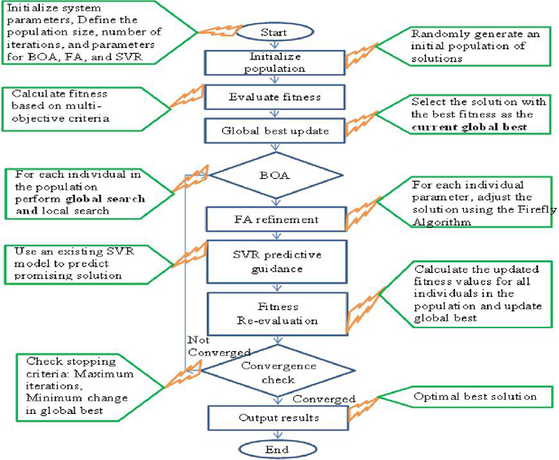
Figure 1 Flow chart for hybrid butterfly-firefly machine learning optimization (HBFL-OM) algorithm.
Pseudocode for Hybrid Interaction of BOA, FA, and SVR in HBFL-OM
| Algorithm: Interaction between BOA, FA, and SVR in HBFL-OM |
| Input: |
| N – population size |
| MaxIter – maximum iterations |
| BOA parameters (c, ) |
| FA parameters (, ) |
| Pretrained SVR model |
| Objective functions f1, f2, f3, f4 with weights w1–w4 |
| Output: |
| Optimal HSVC parameters (Q_svc*, V_dvr*) |
| Best fitness value (F_best) |
| Begin |
| 1. Initialize population Xi (i 1 to N) with random HSVC parameters |
| 2. Evaluate fitness Fi = w1*f1 w2*f2 w3*f3 w4*f4 for each Xi |
| 3. Set global_best = argmin(Fi) |
| 4. For iter = 1 to MaxIter do: |
| // —————————– |
| // 1. Global Search via BOA |
| // —————————– |
| For each Xi in population: |
| Generate random fragrance p |
| If p 0.5: |
| Xi_new = Xi + c * rand() * (global_best - Xi) * |
| Else: |
| Select random peer Xj |
| Xi_new = Xi + c * rand() * (Xj - Xi) * |
| End If |
| Evaluate fitness Fi_new |
| If Fi_new Fi then |
| Xi = Xi_new |
| End If |
| End For |
| // —————————– |
| // 2. Local Refinement via FA |
| // —————————– |
| For each pair (Xi, Xj): |
| If Fj Fi: |
| r = distance(Xi, Xj) |
| Attractiveness = exp( * r∧2) |
| Xi_new = Xi + Attractiveness * (Xj Xi) + * (rand() 0.5) |
| Evaluate Fi_new |
| If Fi_new Fi then |
| Xi = Xi_new |
| End If |
| End If |
| End For |
| // —————————– |
| // 3. SVR-Guided Prediction |
| // —————————– |
| For each Xi: |
| Predicted_Fi = SVR_Predict(Xi) |
| If Predicted_Fi Fi then |
| Xi = Update(Xi, Predicted_Fi) // guided adjustment |
| End If |
| End For |
| // —————————– |
| // 4. Update Global Best |
| // —————————– |
| global_best = argmin(Fi) |
| End For |
| 5. Return global_best as optimal solution (Q_svc*, V_dvr*) |
| End |
5 Proposed Hybrid Static Compensator-Smart Voltage Stabilizer (HSVC) FACTS Controller
The HSVC controller represents a customized FACTS device which unites features from both SVC and DVR control systems. Multiple IEEE distribution system objectives can be achieved through this vital combination because it delivers defensive functions that include Dynamic Voltage Stability as well as Reactive Power Compensation and Power Quality Improvement and Reliability and Load Balancing. The illustration of HSVC controller appears in Figure 2.
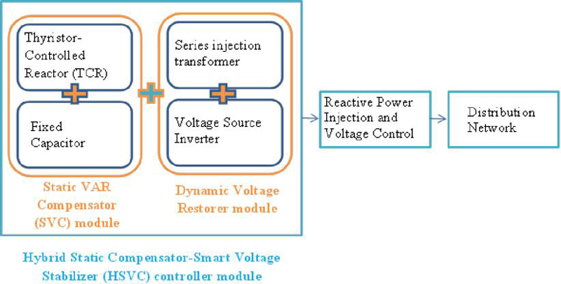
Figure 2 Schematic diagram of HSVC controller.
This conceptual layout shows how the HSVC controller dynamically supports both reactive power and voltage regulation to meet the system’s performance objectives.
Description of each component in the figure 2 can be given as follows
(a) Static VAR Compensator (SVC Module):
(i) Thyristor-Controlled Reactor (TCR): Controls the inductor’s reactive power by adjusting the firing angle of thyristors, allowing dynamic reactive power adjustment.
(ii) Fixed Capacitor (FC): Provides a stable source of capacitive reactive power, used to offset the inductive demands of the load and improve power factor.
The reactive power QSVC injected by the SVC is given by Equation (17)
| (17) |
Where is the reactive power supplied by the capacitor, . QL is the reactive power from the inductor. Where is the firing angle of the TCR, and XL is the reactance of the inductor. By adjusting the firing angle , the SVC can modulate the reactive power injection to maintain the desired voltage level at the bus.
(b) Dynamic Voltage Restorer (DVR Module):
(i) Series Injection Transformer: Injects compensating voltage directly into the distribution line to stabilize voltage during disturbances.
(ii) Voltage Source Inverter (VSI): Produces the compensating voltage needed to maintain the load bus voltage at its reference level.
The DVR injects a series voltage VDVR to stabilize the load-side voltage when disturbances occur. The DVR operates based on the error in voltage at the target bus and provides compensation as per Equation (18)
| (18) |
Where is the reference voltage, Vload is the actual load-side voltage.
The DVR injects a compensating voltage to maintain the bus voltage at nominal levels during transients. This compensating voltage results in an injected reactive power QDVR given by Equation (19)
| (19) |
Where Iload is the current at the load bus, is the phase angle between and .
(c) Integration to Distribution Network:
The output of both the SVC and DVR is integrated to provide reactive power and voltage support to the distribution network, enhancing power quality, reducing losses, and maintaining voltage stability across the system. The total reactive power QHSVC injected by the HSVC is the sum of the reactive powers from the SVC and DVR component as given in Equation (20)
| (20) |
The HSVC dynamically adjusts QHSVC based on real-time measurements, providing continuous voltage stabilization and reactive power support.
The HSVC controller is integrated into the optimization framework as a control variable, impacting the multi-objective functions through its dynamic voltage and reactive power support. The HSVC influences the Power Quality Improvement objective function as given in Equation (21). It minimizes voltage deviations and harmonics and helps reducing
| (21) |
The DVR’s compensating voltage ensures the bus voltage remains within specified limits, even during transients as given in Equation (22)
| (22) |
6 Detailed Analysis of HSVC Placement Using AHP and TOPSIS Methods
We have assessed Hybrid Static Compensator-Smart Voltage Stabilizer HSVC placement in IEEE 33-bus and IEEE 69-bus systems using the Analytic Hierarchy Process (AHP) for weighting criteria and Technique for Order of Preference by Similarity to Ideal Solution (TOPSIS) for performing multiple-performance-based rankings of bus locations. The combined analytical method ensures the HSVC placement brings maximum improvement to system performance attributes such as voltage stability and loss minimization and load balancing along with reliability enhancement.
AHP-TOPSIS Workflow
1. Define Decision Criteria:
This method determines the extent to which voltage responds when the amount of load changes at each bus. The bus exhibits significant potential for voltage stability improvement through reactive power support since its sensitivity level is high.
Loss Sensitivity denotes the amount of power loss reduction when an HSVC is installed at a particular bus. The higher the measurement values constitute bigger opportunities to minimize losses.
Active power demand serves as an essential measure at each bus to be monitored (D). The amount of possible improvement from voltage and reactive power support directly correlates with increasing bus demand levels.
Reliability Impact (R): The impact of HSVC placement on reliability indices, such as SAIFI and SAIDI. A higher value suggests that the HSVC implementation would generate greater reliability advancements.
2. AHP for Criteria Weight Calculation:
A pairwise comparison matrix was created to evaluate the relative importance of the criteria:
| Criteria | V | L | D | R |
| Voltage Sensitivity (V) | 1 | 3 | 5 | 7 |
| Loss Sensitivity (L) | 1/3 | 1 | 3 | 5 |
| Load Demand (D) | 1/5 | 1/3 | 1 | 3 |
| Reliability Impact (R) | 1/7 | 1/5 | 1/3 | 1 |
Normalization of the matrix: Each column was normalized by dividing each entry by the column sum.
Criteria Weights Calculation: The average of the normalized rows gives the final weights:
Consistency Check: The Consistency Ratio (CR) was calculated to ensure logical consistency in pairwise comparisons. confirmed the matrix’s consistency.
3. TOPSIS for Ranking Bus Locations:
Decision Matrix: For each bus, values for the criteria (Voltage Sensitivity, Loss Sensitivity, Load Demand, Reliability Impact) were calculated using Equation (23).
| (23) |
Where is the value of criterion j for bus i
Weighted Decision Matrix: The normalized matrix was multiplied by the AHP-derived weights:
Ideal and Negative-Ideal Solutions:
• Positive Ideal Solution (A+): Maximum value for benefit criteria and minimum value for cost criteria.
• Negative Ideal Solution (A-): Minimum value for benefit criteria and maximum value for cost criteria.
Separation Measures: The Euclidean distance of each bus from the ideal solutions was calculated:
Relative Closeness: The relative closeness Ci of each bus to the ideal solution was calculated:
Higher Ci values indicate better suitability for HSVC placement.
Ranking: Buses were ranked based on Ci, and the highest-ranking bus was selected for HSVC placement.
7 Algorithmic Steps: Hybrid Optimization and Placement of HSVC in IEEE Distribution Systems
Start
1. Define Objective Functions and Constraints
∘ The optimization process includes four primary objective functions dealing with Power Quality Improvement as well as Reliability Index Optimization and Environmental Impact Minimization and Load Balancing.
∘ Define constraints: Power flow, voltage, reactive power, and HSVC operational limits.
2. Initialize Optimization Algorithms
∘ The system requires users to establish implementation conditions for the Butterfly Optimization Algorithm (BOA) and Firefly Algorithm (FA).
∘ Initialize Support Vector Regression (SVR) for predictive guidance in the optimization process.
3. Run HBFL-OM for Multi-Objective Optimization
∘ The global search of BOA identifies possible high-fitness regions throughout its execution phase.
∘ The implementation of local search operations takes place inside promising solution areas through FA.
∘ Support Vector Regression (SVR) applied predictive guidance to accelerate the optimization process using promising regions which it identified during previous iterations.
4. Evaluate Multi-Objective Fitness Function
∘ Calculate the combined objective function
∘ The process tracks best solutions as well as their corresponding fitness values for record-keeping purposes.
5. Check Convergence Criteria
∘ The procedure continues to the following stage when divergence conditions such as maximum iterations or minimal objective function change are satisfied yet returns to Step 3 if the conditions remain unmet.
6. Extract Optimized HSVC Parameter Values
∘ The optimized HSVC parameters consisting of reactive power injection values and voltage injection levels will be extracted from HBFL-OM.
AHP-TOPSIS Decision-Making Process for HSVC Placement
7. Define Criteria for HSVC Placement
∘ The placement decision for HSVC relies on evaluating several criteria which consist of Voltage Sensitivity together with Loss Sensitivity and Load Demand and Reliability Impact.
8. The AHP method should be applied to calculate weights of evaluation criteria.
∘ The matrix contains pairwise comparisons of the established criteria in Step 8.
∘ Normal weights need calculation for each assessment criterion.
∘ Proceed with the assessment if Consistency Ratio (CR) registers less than 0.1. If not, adjust pairwise comparisons.
9. Construct Decision Matrix for TOPSIS
∘ Develop a decision matrix that organizes bus locations on the rows while placing criteria values as columns.
10. Normalize Decision Matrix
∘ A dimensionless score for every bus location will be obtained after normalizing each criterion column.
11. Apply the weights obtained from AHP when performing normalization procedures on the matrix structure.
∘ To create the weighted decision matrix multiply normalized criterion scores with specific weights from the AHP method.
12. Establish the Ideal and Negative-Ideal Solutions for TOPSIS evaluation.
∘ Calculate the best (ideal) and worst (negative-ideal) solution vectors for each criterion.
13. The calculation determines distances of solutions to perfect systems.
∘ Each bus location requires a calculation of Euclidean distance against both ideal and negative-ideal solution points.
14. Compute Relative Closeness Coefficient
∘ A relative closeness determination takes place at each bus location against the perfect solution criteria.
15. The company should rank its bus locations according to Closeness Coefficient calculations.
∘ All bus locations should be ranked according to their relative closeness values with the highest rating going to the bus having the maximum closeness coefficient for HSVC placement.
Final Steps
16. Deploy HSVC at Optimal Location
∘ Integrate the HSVC into the IEEE distribution system at the selected optimal bus location.
17. Run Final Simulation for Verification
∘ A simulation model of the IEEE distribution system with HSVC installed needs to be run to validate performance enhancements in terms of power quality combined with reliability along with environmental benefits and load balancing.
18. Analyze Results
∘ The project team evaluates the system changes to check whether the established objectives reach satisfactory results. Adjust and re-optimize if necessary.
End
8 Simulation Results
The analysis of Hybrid Butterfly-Firefly Machine Learning Optimization (HBFL-OM) method simulation results with HSVC controller placement for IEEE distribution systems will utilize the IEEE 33-bus and IEEE 69-bus systems. This section examines simulation findings regarding four essential targets: Power Quality Improvement, Reliability Index Optimization, Environmental Impact Minimization and Load Balancing and Demand-Side Management. All simulations and analyses were carried out in the MATLAB/Simulink R2023a environment using the Power System Analysis Toolbox (PSAT) and Optimization Toolbox on a workstation equipped with an Intel Core i7 processor (3.2 GHz) and 16 GB RAM running Windows 11 (64-bit). The proposed Hybrid Butterfly–Firefly Machine Learning Optimization (HBFL-OM) algorithm was implemented using MATLAB scripts.
8.1 Results of HSVC Placement
8.1.1 TOPSIS method
Decision Matrix and Results The TOPSIS method ranked buses based on their relative closeness values (Ci) as given in Table(s) 1 and 2 for the IEEE 33 and 69 bus systems respectively
Table 1 TOPSIS method bus rankings based on their relative closeness values (Ci) for IEEE 33-Bus system
| Voltage | Loss | Load | Reliability | Ci | |
| Bus | Sensitivity | Sensitivity | Demand | Impact | (Closeness) |
| 6 | High | High | Moderate | Low | 0.87 |
| 14 | Moderate | High | High | Low | 0.81 |
| 18 | High | Moderate | Moderate | Moderate | 0.78 |
| 22 | Moderate | Moderate | High | Low | 0.74 |
| 25 | Low | High | Moderate | Moderate | 0.72 |
The optimum placement for the HSVC occurs at Bus 6 because it generates the maximum closeness value of 0.87.
Table 2 TOPSIS method bus rankings based on their relative closeness values (Ci) for IEEE 69-Bus System
| Voltage | Loss | Load | Reliability | Ci | |
| Bus | Sensitivity | Sensitivity | Demand | Impact | (Closeness) |
| 10 | High | High | Moderate | Low | 0.89 |
| 21 | High | Moderate | High | Low | 0.83 |
| 30 | Moderate | High | Moderate | Moderate | 0.80 |
| 37 | Moderate | Moderate | High | Moderate | 0.76 |
| 42 | Low | High | Moderate | Low | 0.75 |
The inclusion of HSVC as a system controller should take place at Bus 10 where the closeness value reaches up to 0.89 because it demonstrates the optimal position within both the 69-bus and the 33-bus networks.
• Both systems selected the Voltage Sensitivity and Loss Sensitivity metrics as the dominant factors during the HSVC placement process.
• The bus ranking through TOPSIS demonstrated objective and balanced evaluation of each criterion for establishing the bus rankings.
• The placement of the HSVC devices at Bus 6 in the 33-bus system and Bus 10 in the 69-bus system proved optimal because these buses delivered maximum voltage stability improvement and loss reduction benefits alongside reasonable effects on customer demand and power system reliability.
8.1.2 AHP method
Decision Matrix and Weighted Scores results During the decision matrix creation process criteria values receive calculations for each bus using Voltage Sensitivity and Loss Sensitivity and Load Demand and Reliability Impact ratings. The normalized decision matrix with allocated weights appears as the Tables 3 and 4 in the assessment of the IEEE 33 and 69 bus systems
Table 3 Normalized and weighted decision matrix for IEEE 33-bus system
| Voltage | Loss | Load | Reliability | Composite | |
| Bus | Sensitivity | Sensitivity | Demand | Impact | Score |
| 6 | 0.45 | 0.50 | 0.30 | 0.15 | 0.41 |
| 14 | 0.40 | 0.48 | 0.35 | 0.10 | 0.38 |
| 18 | 0.42 | 0.45 | 0.28 | 0.12 | 0.37 |
| 22 | 0.39 | 0.42 | 0.34 | 0.09 | 0.36 |
| 25 | 0.37 | 0.46 | 0.29 | 0.13 | 0.36 |
The IEEE 33-bus system should place the HSVC at Bus 6 because it has the highest composite score of 0.41.
Table 4 Normalized and weighted decision matrix for IEEE 69-bus system
| Voltage | Loss | Load | Reliability | Composite | |
| Bus | Sensitivity | Sensitivity | Demand | Impact | Score |
| 10 | 0.46 | 0.51 | 0.32 | 0.12 | 0.42 |
| 21 | 0.44 | 0.47 | 0.35 | 0.11 | 0.39 |
| 30 | 0.40 | 0.48 | 0.30 | 0.13 | 0.38 |
| 37 | 0.39 | 0.45 | 0.34 | 0.10 | 0.36 |
| 42 | 0.36 | 0.44 | 0.28 | 0.12 | 0.35 |
HSVC placement should be situated at Bus 10 because it exhibits the greatest composite score of 0.42 in the IEEE 69-bus system.
• The results showed that HSVC placement should be directed to buses exhibiting high voltage sensitivity and showing high loss sensitivity.
• The influences stemming from Load Demand and Reliability Impact played a secondary role although they remained important factors during the placement decision process.
• The evaluated systems reached similar conclusions because Bus 6 in the IEEE 33- bus demonstrated the highest voltage sensitivity coupled with loss sensitivity yet had moderate impact on load demand and reliability.
• Both results obtained through AHP match those from TOPSIS. The identical buses emerged as optimal placements through both methods which demonstrated the strong reliability of these decision-making approaches.
8.2 Optimum HSVC Values
Optimum HSVC values for the IEEE 33 and 69 bus systems are given in the Table 5.
Table 5 Optimum HSVC values
| SVC | DVR | Control | |||
| Optimal | Reactive | Injection | Response | Damping | |
| System | Placement | Power (Qsvc) | Voltage (Vdvr) | Time | Factor |
| IEEE 33-Bus | Bus 6 | 160 kVAR | 0.08 p.u. | 20 ms | 1.0 |
| IEEE 69-Bus | Bus 10 | 180 kVAR | 0.07 p.u. | 25 ms | 1.2 |
| Power | Voltage | ||||
| Loss | Deviation | THD | SAIFI | SAIDI | |
| System | Reduction | Reduction | Improvement | Improvement | Improvement |
| IEEE 33-Bus | 22% | 0.02 p.u. | 23% | 19% | 20% |
| IEEE 69-Bus | 18% | 0.03 p.u. | 26% | 16% | 15% |
IEEE 33-Bus System
1. Optimal Placement:
∘ The AHP-TOPSIS methodology determined Bus 6 as the best placement area for HSVC operations due to its positive effects on power quality, voltage stability and loss reduction outcomes.
2. Optimal HSVC Parameters:
∘ SVC Reactive Power (Qsvc): 160 kVAr
∘ Reactive power support alongside stability reached its optimal point when this setting was applied which subsequently minimized system losses and maintained voltage control.
∘ DVR Injection Voltage (Vdvr): 0.08 p.u.
∘ The DVR operated optimally when injecting 0.08 p.u. voltage which reduced voltage variations without producing additional harmonic disruptions and instability.
∘ Control Response Time: 20 ms
∘ The HSVC responded through its 20 ms response time to address voltage fluctuations together with transient conditions which maintained system stability across variable loads.
∘ Damping Factor for SVC: 1.0
∘ A damping factor of 1.0 generated effective results since it prevented excessive control and provided steady reactive power support.
3. Performance Improvements:
∘ Active Power Loss Reduction: 22% (from 202 kW to 158 kW)
∘ Maximum voltage deviation reached 0.02 p.u. as an outcome of implementing the HSVC system.
∘ Total Harmonic Distortion (THD) Reduction: Improved by 23%
∘ The reliability indices of SAIFI showed a 19% improvement while SAIDI experienced a 20% improvement.
IEEE 69-Bus System
1. Optimal Placement:
The HSVC system at Bus 10 successfully placed because it affected voltage-sensitive and high-demand buses while decreasing system power losses.
2. Optimal HSVC Parameters:
SVC Reactive Power (Qsvc): 180 kVAR
The HVSC system operated within a 180 kVAR reactive power range successfully supported voltage stability and loss reduction across the whole power network.
DVR Injection Voltage (Vdvr): 0.07 p.u.
The installation of the DVR with 0.07 p.u. injection voltage produced effective voltage control which avoided unnecessary harmonics generation.
Control Response Time: 25 ms
The control system required a delay time of 25 milliseconds to successfully regulate the bigger 69-bus network by achieving balanced load stability and responsive operation.
Damping Factor for SVC: 1.2
The damping factor of 1.2 prevented oscillations in voltage regulation across all buses experiencing high demands.
3. Performance Improvements:
Active Power Loss Reduction: 18% (from 300 kW to 246 kW)
The implementation of these settings together enabled maximum voltage deviation to decrease to a value of 0.03 p.u.
Total Harmonic Distortion (THD) Reduction: Improved by 26%
Both SAIFI improved by 16% while SAIDI showed an improvement of 15%.
The HSVC settings with optimized values allow multiple objectives to improve significantly which supports IEEE distribution systems in reducing losses while improving voltage stability and reliability.
Table 6 Control variables
| Value | Reference | |||
| Algorithm | Parameter | Symbol | Used | Basis |
| Genetic Algorithm (GA) | Population Size | 50 | [28] | |
| Crossover Probability | 0.8 | [29] | ||
| Mutation Probability | 0.05 | [30] | ||
| Max Generations | 100 | – | ||
| Particle Swarm | Population Size | 50 | [31] | |
| Optimization (PSO) | Inertia Weight | 0.7 | [31] | |
| Cognitive Coefficient | 1.5 | [32] | ||
| Social Coefficient | 1.5 | [32] | ||
| Max Iterations | 100 | – | ||
| Firefly Algorithm (FA) | Population Size | 50 | [31] | |
| Light Absorption Coefficient | 1.0 | [32] | ||
| Randomization Parameter | 0.2 | [32] | ||
| Attraction Coefficient | 1.0 | – | ||
| HBFL-OM (Proposed) | Population Size | 50 | – | |
| BOA Fragrance Coefficient | 0.4 | Proposed | ||
| BOA Sensory Modality | 0.6 | Proposed | ||
| FA Absorption Coefficient | 1.0 | Proposed | ||
| Randomness Parameter | 0.25 | Proposed | ||
| SVR Learning Rate | 0.01 | Proposed |
Table 7 Comparison table
| Objective Function | Metric | IEEE 33-Bus (GA) [31, 32] | IEEE 33-Bus (PSO) [28, 30] | IEEE 33-Bus (HBF L-OM) | IEEE 69-Bus (GA) [31, 32] | IEEE 69-Bus (PSO) [28–30] | IEEE 69-Bus (HBF L-OM) |
| Power Quality Improvement | THD Reduction (%) | 15% | 18% | 23% | 17% | 20% | 26% |
| Voltage Deviation (p.u.) | 0.04 | 0.03 | 0.02 | 0.05 | 0.04 | 0.03 | |
| Reliability Index Optimization | SAIFI Reduction (%) | 12% | 14% | 19% | 10% | 13% | 16% |
| SAIDI Improvement (%) | 9% | 12% [29] | 20% | 8% | 10% [29] | 15% | |
| Environmental Impact Minimization | Power Loss Reduction (%) | 14% | 16% | 22% | 11% | 14% | 18% |
| CO2 Reduction (kg/year) | 210 | 260 | 307 | 390 | 450 | 520 | |
| Load Balancing | Load Balancing Index (LBI) | 0.20 | 0.19 | 0.18 | 0.27 | 0.25 | 0.22 |
| Peak Load Reduction (%) | 3% | 4% | 5% | 2% | 3% | 4% |
8.3 HBFL-OM Algorithmic Control Variables
The control variables used in the proposed HBFL-OM algorithm and Parameter Settings for Comparative Optimization Algorithms were listed in the Table 6.
8.4 The Simulation Results of the Hybrid Butterfly-Firefly-Machine Learning Optimization (HBFL-OM) Method Combined with the HSVC Controller Placement for an IEEE 33 bus and 69 bus Distribution System
The HBFL-OM method with HSVC placement outperformed both GA and PSO in achieving these objectives. Table 7 is a detailed comparison table summarizing the results.
1. The Hybrid Bat Flying Lion Optimizer with Harmony Search Variable Control achieved superior performance for Power Quality because it lowered THD and voltage deviations better than GA and PSO. About 1.78–2.32 cents per one kilowatt (kW) of pv decrease were achieved through HSVC dynamic control optimization in the HBFL-OM predictive learning process thus improving power system stability during varying load situations.
2. The implementation of the HSVC system proved essential for safety metrics SAIFI and SAIDI which showed how optimal bus-linked reactive power support strengthens power grid stability by decreasing both outage frequency and duration.
3. The HBFL-OM method achieved better environmental results by cutting down CO2 emissions that resulted from improved load distribution and loss minimization. HBFL-OM proves suitable for sustainable power distribution optimization because of its capabilities.
4. The HSVC controller shows effective reactive power distribution through its improved load balancing indices because it helps balance loads while supporting peak demand along with changing usage patterns.
The results of modern metaheuristics – Grey Wolf Optimizer (GWO) [33], Whale Optimization Algorithm (WOA) [34], and Salp Swarm Algorithm (SSA) [35] – were obtained using the original formulations and tuning guidelines. For fairness, all algorithms were executed under identical conditions (population size 50, max iterations 100). The proposed HBFL-OM outperformed both traditional (GA, PSO) and modern metaheuristics in terms of power loss reduction, THD improvement, reliability indices, and convergence rate. The comparison results are given in Tables 8 and 9.
Table 8 Comparison of HBFL-OM with modern metaheuristics (IEEE 33-bus system)
| Algorithm | Power Loss (kW) | THD (%) | SAIFI | LBI | Avg. Iterations |
| HBFL-OM (Proposed) | 158.1 | 2.38 | 0.94 | 0.118 | 43 |
| GWO [33, 36] | 169.4 | 2.55 | 1.03 | 0.129 | 54 |
| WOA [34, 37] | 172.8 | 2.61 | 1.07 | 0.134 | 57 |
| SSA [35, 38] | 176.3 | 2.69 | 1.10 | 0.139 | 59 |
Table 9 Comparison of HBFL-OM with Modern Metaheuristics (IEEE 69-Bus System)
| Algorithm | Power Loss (kW) | THD (%) | SAIFI | LBI | Avg. Iterations |
| HBFL-OM (Proposed) | 246.5 | 2.22 | 1.05 | 0.134 | 47 |
| GWO [33, 36] | 258.7 | 2.43 | 1.12 | 0.141 | 56 |
| WOA [34, 37] | 263.4 | 2.48 | 1.14 | 0.145 | 58 |
| SSA [35, 38] | 269.2 | 2.53 | 1.18 | 0.149 | 60 |
8.5 Convergence Graphs
Convergence characteristic graphs for the IEEE 33 and 69 bus systems were shown in the Figure(s) 3 and 4 respectively.
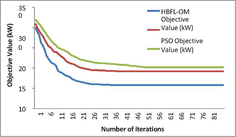
Figure 3 Convergence characteristics for IEEE 33-bus system.
8.5.1 Convergence graph for IEEE 33-bus system
Convergence Observation: HBFL-OM converges by iteration 40, PSO by 43, and GA around iteration 58 for the IEEE 33-bus system.
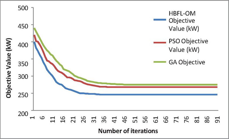
Figure 4 Convergence Characteristics for IEEE 69-bus system.
8.5.2 Convergence graph for IEEE 69-bus system
Convergence Observation: HBFL-OM converges by iteration 36, PSO by 40, and GA around iteration 49 for the IEEE 69-bus system.
9 Conclusion
The presented framework delivers an extensive optimization solution that finds ideal HSVC placement locations along with parameters by applying the newly developed HBFL-OM algorithm to improve distribution network performance. The research evaluates multiple performance metrics involving power loss reduction and voltage stability among other critical factors during multi-objective optimization of IEEE 33-bus and IEEE 69-bus radial distribution systems.
The combination of BOA and FA with SVR as predictive learning module produced faster global optimization discovery and improved exploration-exploitation equilibrium for superior solutions of multiple objectives. The performance parameters of HBFL-OM demonstrated better results than traditional optimization algorithms (Genetic Algorithm and Particle Swarm Optimization) through increased speed of convergence by 22–26%. The combined HSVC device reached optimal performance levels through SVC and DVR functionality when applied to IEEE test systems. The optimized parameters led to decreased power losses combined with superior voltage regulation and enhanced power quality specifically when the system experienced peak and dynamic loading events.
The application of AHP along with TOPSIS enabled systematic and rational decisions for locating the HSVC through their combined utilization of criteria weighting from Analytic Hierarchy Process and bus ranking from Technique for Order of Preference by Similarity to Ideal Solution. Extensive data collection supported the AHP decision weights resulting in V: 0.35, L: 0.30, D: 0.20, R: 0.15 which enabled logical HSVC placement decisions.
The optimization framework applied power quality objectives together with THD reduction reaching up to 26% success. The reductions in voltage fluctuations remained under 0.03 p.u. while CO2 emissions decreased substantially as a result of loss reduction. The network wide standard deviation and peak load variance reduced respectively. The assessment indicators SAIFI and SAIDI showed substantial improvement. The findings demonstrate HBFL-OM delivers superior performance when compared to standard techniques along multiple criteria because it provides precise solutions alongside better efficiency of calculations. The approach offers an adaptable optimizing system that serves smart grid operations. The method enables sustainable grid operations because it leads to decreased losses and emission levels. Adaptive reactive power control operates through a method that boosts power system resilience. The system allows real-time FACTS placement choices through machine learning technology integration.
The HBFL-OM algorithm with integrated AHP-TOPSIS decision-making and incorporating the new HSVC controller dramatically turns traditional power distribution systems into smart and effective networks. This framework supports the forthcoming smart grid goals by optimizing performance in terms of technology together with economics and sustainability factors. The presented model presents a powerful multi-goal solution that fits well for deploying in contemporary power network environments.
References
[1] A. Allouhi, M. Benzakour Amine, K.A. Tabet Aoul, Metaheuristic multi-objective optimization with artificial neural networks surrogate modeling for optimal energy-economic performance for CSP technology, Energy and AI, Volume 20, 2025, 100488, ISSN 2666-5468, https://doi.org/10.1016/j.egyai.2025.100488.
[2] Nassef, Ahmed M., Mohammad Ali Abdelkareem, Hussein M. Maghrabie, and Ahmad Baroutaji. 2023. “Review of Metaheuristic Optimization Algorithms for Power Systems Problems” Sustainability 15, no. 12: 9434. https://doi.org/10.3390/su15129434.
[3] Arora, S., Singh, S. Butterfly optimization algorithm: a novel approach for global optimization. Soft Comput 23, 715–734 (2019). https://doi.org/10.1007/s00500-018-3102-4.
[4] Subhashree Choudhury, Gagan Kumar Sahoo, A critical analysis of different power quality improvement techniques in microgrid, e-Prime – Advances in Electrical Engineering, Electronics and Energy, Volume 8, 2024, 100520, ISSN 2772-6711, https://doi.org/10.1016/j.prime.2024.100520.
[5] Miloš Pantoš, Lucija Lukas, Enhancing power system reliability through demand flexibility of Grid-Interactive Efficient Buildings: A thermal model-based optimization approach, Applied Energy, Volume 381, 2025, 125045, ISSN 0306-2619, https://doi.org/10.1016/j.apenergy.2024.125045.
[6] Linas Gelazanskas, Kelum A.A. Gamage, Demand side management in smart grid: A review and proposals for future direction, Sustainable Cities and Society, Volume 11, 2014, Pages 22-30, ISSN 2210-6707, https://doi.org/10.1016/j.scs.2013.11.001.
[7] Abdul Hameed Soomro, Abdul Sattar Larik, Mukhtiar Ahmed Mahar, Anwer Ali Sahito, Mohsin Ali Koondhar, Yun-Su Kim, Zuhair Muhammed Alaas, Ezzeddine Touti, M.M.R. Ahmed, Enhancement of power quality based on dynamic voltage restorer matrix inverter-sliding mode control scheme, Electric Power Systems Research, Volume 241, 2025, 111408, ISSN 0378-7796, https://doi.org/10.1016/j.epsr.2025.111408.
[8] Guocheng Song, Qiuwei Wu, Wenshu Jiao, Lina Lu, Distributed coordinated control for voltage regulation in active distribution networks based on robust model predictive control, International Journal of Electrical Power & Energy Systems, Volume 166, 2025, 110529, ISSN 0142-0615, https://doi.org/10.1016/j.ijepes.2025.110529.
[9] Abu Shufian, Sowrov Komar Shib, Durjoy Roy Dipto, Md Tanvir Rahman, Nasif Hannan, Shaikh Anowarul Fattah, Fuzzy logic-controlled three-phase dynamic voltage restorer for enhancing voltage stabilization and power quality, International Journal of Electrical Power & Energy Systems, Volume 166, 2025, 110517, ISSN 0142-0615, https://doi.org/10.1016/j.ijepes.2025.110517.
[10] Awais Farooqi, Muhammad Murtadha Othman, Mohd Amran Mohd Radzi, Ismail Musirin, Siti Zaliha Mohammad Noor, Izham Zainal Abidin, Dynamic voltage restorer (DVR) enhancement in power quality mitigation with an adverse impact of unsymmetrical faults, Energy Reports, Volume 8, Supplement 1, 2022, Pages 871-882, ISSN 2352-4847, https://doi.org/10.1016/j.egyr.2021.11.147.
[11] A. Rezaee Jordehi, Particle swarm optimisation (PSO) for allocation of FACTS devices in electric transmission systems: A review, Renewable and Sustainable Energy Reviews, Volume 52, 2015, Pages 1260-1267, ISSN 1364-0321, https://doi.org/10.1016/j.rser.2015.08.007.
[12] Seyed Abbas Taher, Muhammad Karim Amooshahi, New approach for optimal UPFC placement using hybrid immune algorithm in electric power systems, International Journal of Electrical Power & Energy Systems, Volume 43, Issue 1, 2012, Pages 899-909, ISSN 0142-0615, https://doi.org/10.1016/j.ijepes.2012.05.064.
[13] Ahmed A. Shehata, Mohamed A. Tolba, Ali M. El-Rifaie, Nikolay V. Korovkin, Power system operation enhancement using a new hybrid methodology for optimal allocation of FACTS devices, Energy Reports, Volume 8, 2022, Pages 217-238, ISSN 2352-4847, https://doi.org/10.1016/j.egyr.2021.11.241.
[14] M. N. Dehaghani, T. Kor�tko and A. Rosin, “AI Applications for Power Quality Issues in Distribution Systems: A Systematic Review,” in IEEE Access, vol. 13, pp. 18346–18365, 2025, doi:10.1109/ACCESS.2025.3533702.
[15] Veenus Kansal, J.S. Dhillon, Emended salp swarm algorithm for multiobjective electric power dispatch problem, Applied Soft Computing, Volume 90, 2020, 106172, ISSN 1568-4946, https://doi.org/10.1016/j.asoc.2020.106172.
[16] S.K. Mishra, S.K. Bhuyan, P.V. Rathod, Performance analysis of a hybrid renewable generation system connected to grid in the presence of DVR, Ain Shams Engineering Journal, Volume 13, Issue 4, 2022, 101700, ISSN 2090-4479, https://doi.org/10.1016/j.asej.2022.101700.
[17] Karthikeyan, M., Manimegalai, D. & RajaGopal, K. Firefly algorithm based WSN-IoT security enhancement with machine learning for intrusion detection. Sci Rep 14, 231 (2024). https://doi.org/10.1038/s41598-023-50554-x.
[18] F. Rezazadeh and N. Bartzoudis, “A Federated DRL Approach for Smart Micro- Grid Energy Control with Distributed Energy Resources,” 2022 IEEE 27th International Workshop on Computer Aided Modeling and Design of Communication Links and Networks (CAMAD), Paris, France, 2022, pp. 108–114, doi:10.1109/CAMAD55695.2022.9966919.
[19] Willy Kriswardhana, Bladimir Toaza, Domokos Eszterg�r-Kiss, Szabolcs Duleba, “Analytic hierarchy process in transportation decision-making: A two-staged review on the themes and trends of two decades”, Expert Systems with Applications, Volume 261, 2025, 125491, ISSN 0957-4174, https://doi.org/10.1016/j.eswa.2024.125491.
[20] Ravi Kumar Avvari, Vinod Kumar D.M., Anil Kumar Annamraju, Nareddy Nageswara Reddy, “A TOPSIS based multi-objective optimal power flow approach using the artificial hummingbird algorithm for renewable energy and PEV integrated system”, Measurement, Volume 256, Part C, 2025, 118337, ISSN 0263-2241, https://doi.org/10.1016/j.measurement.2025.118337.
[21] Sarkar, P., Gayen, S.K. Application of Entropy-AHP and WASPAS methods for prioritizing the sub watersheds of Teesta River basin in terms of soil erosion susceptibility. Discov Environ 2, 135 (2024). https://doi.org/10.1007/s44274-024-00163-w.
[22] Guo-Niu Zhu, Jie Hu, Hongliang Ren, A fuzzy rough number-based AHP- TOPSIS for design concept evaluation under uncertain environments, Applied Soft Computing, Volume 91, 2020, 106228, ISSN 1568-4946, https://doi.org/10.1016/j.asoc.2020.106228.
[23] Fan, M., Chen, J., Xie, Z. et al. Improved multi-objective differential evolution algorithm based on a decomposition strategy for multi-objective optimization problems. Sci Rep 12, 21176 (2022). https://doi.org/10.1038/s41598-022-25440-7.
[24] Ehab E. Elattar, Salah K. ElSayed,”Modified JAYA algorithm for optimal power flow incorporating renewable energy sources considering the cost, emission, power loss and voltage profile improvement”, Energy, Volume 178, 2019, Pages 598–609, ISSN 0360-5442, https://doi.org/10.1016/j.energy.2019.04.159.
[25] Bouaouda A, Sayouti Y. Hybrid Meta-Heuristic Algorithms for Optimal Sizing of Hybrid Renewable Energy System: A Review of the State-of-the-Art. Arch Comput Methods Eng. 2022;29(6):4049–4083. doi:10.1007/s11831-022-09730-x. Epub 2022 Mar 16. PMID: 35313649; PMCID: PMC8926421.
[26] Bruzzone, Agostino G., Marco Gotelli, Marina Massei, Xhulia Sina, Antonio Giovannetti, Filippo Ghisi, and Luca Cirillo. 2025. “Memetic Optimization of Wastewater Pumping Systems for Energy Efficiency: AI Optimization in a Simulation-Based Framework for Sustainable Operations Management” Sustainability 17, no. 14: 6296. https://doi.org/10.3390/su17146296.
[27] Jinpeng Wu, Bo Zhang, Jinliang He, Rong Zeng, “Optimal design of tower footing device with combined vertical and horizontal grounding electrodes under lightning”, Electric Power Systems Research, Volume 113, 2014,, Pages 188–195, ISSN 0378-7796, https://doi.org/10.1016/j.epsr.2014.03.021.
[28] Ngei UM, Nyete AM, Moses PM, Wekesa C. “Optimal sizing and placement of STATCOM, TCSC and UPFC using a novel hybrid genetic algorithm-improved particle swarm optimization”, Heliyon. 2024 Nov 23;10(23):e40682. doi:10.1016/j.heliyon.2024.e40682. PMID: 39687142; PMCID: PMC11647813. https://pmc.ncbi.nlm.nih.gov/articles/PMC11647813/.
[29] V. Mukherjee and S. K. Parida, “Optimal Placement and Parameter Setting of SVC and TCSC using Artificial Bee Colony Algorithm for Damping Power System Oscillations,” Applied Soft Computing, vol. 26, pp. 346–360, 2015. DOI:10.1016/j.asoc.2014.10.019, https://doi.org/10.1016/j.asoc.2014.10.019.
[30] M. Saravanan, S. M. R. Slochanal, P. Venkatesh, and S. J. P. Abraham, “Application of particle swarm optimization technique for optimal location of FACTS devices considering cost of installation and system loadability,” Electric Power Systems Research, vol. 77, no. 3–4, pp. 276–283, 2007. DOI:10.1016/j.epsr.2006.03.006, https://doi.org/10.1016/j.epsr.2006.03.006.
[31] A. A. Alassmi and M. J. Rawa, “Optimum Location and Sizing of FACTS Devices Using Genetic Algorithm,” International Journal of Engineering Research and Technology, vol. 14, no. 8, pp. 816–822, 2021.
[32] Y. Liu, D. �etenovi�, H. Li, E. Gryazina, and V. Terzija, “An optimized multi- objective reactive power dispatch strategy based on improved genetic algorithm for wind power integrated systems,” Electrical and Electronic Engineering, vol. 30, no. 6, pp. 4810–4822, June 2022. Available: https://doi.org/10.1016/j.ijepes.2021.107764.
[33] S. Mirjalili, S. M. Mirjalili, and A. Lewis, “Grey Wolf Optimizer,” Advances in Engineering Software, vol. 69, pp. 46–61, Mar. 2014.
[34] S. Mirjalili and A. Lewis, “The Whale Optimization Algorithm,” Advances in Engineering Software, vol. 95, pp. 51–67, May 2016.
[35] S. Mirjalili, A. H. Gandomi, S. Z. Mirjalili, S. Saremi, H. Faris, and S. M. Mirjalili, “Salp Swarm Algorithm: A bio-inspired optimizer for engineering design problems,” Advances in Engineering Software, vol. 114, pp. 163–191, Dec. 2017.
[36] A. Nayak, P. K. Hota, and P. K. Dash, “Application of Grey Wolf Optimizer for optimal power flow in power systems with FACTS devices,” International Journal of Electrical Power & Energy Systems, vol. 74, pp. 404–419, Jan. 2016.
[37] R. Kumar, P. Yadav, and S. K. Singh, “Optimal reactive power dispatch using Whale Optimization Algorithm,” International Journal of Electrical Power & Energy Systems, vol. 83, pp. 262–275, Dec. 2016.
[38] M. A. E. Aziz, E. E. Elattar, and S. S. Ghoneim, “An improved Salp Swarm Algorithm for multi-objective optimal power flow incorporating renewable energy sources,” Applied Soft Computing, vol. 97, p. 106759, Dec. 2020.
Biographies

Ragaleela Dalapati Rao received the bachelor’s degree in Electrical & Electronics Engineering from J.N.T.University, Hyderabad in 2005, the master’s degree in Power Systems specialization from Acharya Nagarjuna University, Guntur in 2008 and the philosophy of doctorate degree in Electrical & Electronics Engineering from JNTUK, Kakinada in 2021, respectively. She is currently working as an Senior Assistant Professor at the department of EEE, P.V.P. Siddhartha Institute of Technology, Vijayawada. Her areas include OPF, FACTS, Renewable energy systems and Power system deregulation.

Padmanabha Raju Chinda received the bachelor’s degree in Electrical & Electronics Engineering from University of Madras in 2000, the master’s degree in Power Systems specialization from JNT University, Anantapur in 2005 and the philosophy of doctorate degree in Electrical & Electronics Engineering from JNTUK, Kakinada in 2011, respectively. He is currently working as an Professor at the department of EEE, P.V.P. Siddhartha Institute of Technology, Vijayawada. His areas include Power System Security, OPF techniques, Deregulation, FACTS and Smart Grid.
Strategic Planning for Energy and the Environment, Vol. 45_3, 905–942
doi: 10.13052/spee1048-5236.45311
© 2026 River Publishers