Deep Learning Architectures for Advanced Anomaly Detection in Solar Photovoltaic Systems
Musab Bin Khaleeq and Mohammad Sarfraz*
ZHCET, Aligarh Muslim University, Aligarh, India
E-mail: ma.musabali1998@gmail.com; msarfraz@zhcet.ac.in
*Corresponding Author
Received 06 October 2025; Accepted 25 February 2026
Abstract
Solar photovoltaic (PV) system operation and maintenance are important for achieving global sustainability objectives. Also, the reliability of PV is one thing that has always prevented it from reaching the full product guarantee due to hotspot, diode degradation, shading, and cracks issues. Traditional inspection methods are time-consuming, expensive, and can contain errors, which justifies the development of automation systems. This paper proposes a deep learning-based framework for anomaly detection using high-resolution RGB images, which overcomes the drawbacks of low-resolution grayscale datasets. To improve robustness, a dataset consisting of 20,000 PV module images with eleven fault categories and normal modules was systematically preprocessed by resizing, augmentation, and quality assurance. Six models, namely, CNN model, AlexNet, VGG16, ResNet18, DenseNet, and EfficientNetV2B0, were compared with each other through the evaluation metrics of accuracy, precision, recall, and F1 score. The experimental results show that the RGB transform can greatly benefit feature learning and model generalization. Overall, ResNet18 had the highest accuracy (91.1%) while EfficientNetV2B0 had balanced performance overall metrics. The results highlight Deep-Learning applications with fine quality datasets (i.e., achieving high performances of Anomaly Detection, Predictive Maintenance, and Sustainable Energy Generation).
Keywords: Sustainability, deep learning, solar photovoltaic, anomaly detection, RGB imaging, EfficientNetV2B0, ResNet18, VGG16, DenseNet.
1 Introduction and Related Work
1.1 Background and Motivation
The global demand for clean and sustainable energy has accelerated, leading to the fast development of renewable energy technologies, of which solar photovoltaic (PV) systems play a central part. Large-scale installations of photovoltaics have been added to modern electric power systems in growing numbers because of their scalability, environmental benefits, and falling installation costs [1]. Nevertheless, such photovoltaic systems are subject on a regular basis to a diversity of operational anomalies such as cell cracks, diode failures, hotspots, partial shading, and surface soiling. Such defects can cause a significant decrease in the energy output but also lead to faster degradation of the system, increased maintenance costs, and high safety risks [2, 3]. Consequently, to ensure the reliable and continuous operation of PV systems, the use of effective monitoring and early fault detection mechanisms will be required to ensure reliable operation. Nevertheless, the large spatial scale and distributed configuration of the modern solar farms present a disturbing challenge for the reliable inspection and maintenance [4].
1.2 Traditional Monitoring Methods and Their Limitations
Traditional photovoltaic inspection methodologies predominantly depend upon the manual visual examination and electrical measurement-based procedure and monitoring systems. These methods can detect some modes of fault; they have a number of limitations [5]. Manual inspection is so laborious, time-consuming, and prone to human subjectivity that it is unsuitable for large-scale deployments. Electrical and sensor-based approaches often require supportive hardware, add to system complexity, and can ignore defects on the surface that are not immediately affecting electrical parameters [5, 6]. As photovoltaic installations are continuously increased in size and scale, this traditional approach becomes inadequate in fault detection that is scalable and reliable in terms of cost and time [3, 4, 5, 6, 7]. Accordingly, there has been an increasing push to go for automated and intelligent monitoring methodologies.
1.3 Deep Learning–Based Anomaly Detection in PV Systems
Recent developments in artificial intelligence (AI) and machine learning (ML) have provided a very useful basis for the data-driven approaches of automated anomaly detection in photovoltaic (PV) systems. Machine learning methods can detect a variation from normal operating behavior by learning complex patterns in historical data. Classical ML techniques like Support Vector Machines (SVMs), Artificial Neural Networks (ANNs), autoencoders, and Long Short Term Memory (LSTMs) networks have been explored previously for PV faults detection, especially in time series and electrical signals analysis [8].
In very recent developments, deep learning methodologies have been shown to be robust in the application of vision-based photovoltaic monitoring tasks, in particular Convolutional Neural Networks (CNNs). CNN-based frameworks are well-suited for analysing spatial patterns within image data and hence enabling the effective detection of surface anomalies based on thermal as well as electroluminescence and aerial imagery. Transfer learning methods based on pretrained architectures, like AlexNet, VGG, ResNet, DenseNet, and EfficientNet, have further enhanced the detection accuracy by making use of huge and vast feature representations acquired from large-scale image datasets [9, 10].
However, there is often a limit to the size of the trained networks (known as deep learning models) because of the size and quality of the labeled data. Numerous current studies are based on low-resolution grayscale images, which delay visualization of fine-grained defects such as microcracks, local hotspots, and partial shading. This limitation impacts the human interpretation and the automated feature extraction adversely [3, 4, 5, 6, 7, 8, 9, 10, 11].
1.4 Recent Works
Recent studies have been focusing more on how to improve the photovoltaic anomaly detection, such as improving data representations, applying lightweight deep learning architectures, and formulating real-world deployment strategies [12]. Empirical investigations have repeatedly validated the good performance of convolutional neural network (CNN) architectures in application to RGB aerial imagery for the detection of surface defects, therefore highlighting the information-giving benefits imparted by chromatic and textural information with respect to monocolour representations [12, 13].
Subsequent investigations have focused on hybrid frameworks and prevention welding as a way to deep learning and adjusting adaptation procedures or incorporating transformer-based architectures to upgrade generalisation and robustness more than a wide range of environmental conditions [14].
Concurrently, the current learning has been reporting back multimodal inspection methodologies combining visual and thermal data as well as computationally efficient models, modified for edge deployment or real-time deployment. Although these methods are producing encouraging outcomes, many of these studies are limited to single model assessments, a limited class of defects, or expensive sensing technologies, thus again establishing the need for additional work to develop scalable and cost-effective methods that can be based entirely on common RGB imagery [15, 16].
1.5 Research Gap
Despite the progress achieved by recent deep learning–based approaches, several gaps remain in the existing literature. First, many studies rely on low-resolution or modality-specific datasets, limiting the extraction of rich spatial and color features. [3] Second, comparative evaluations across multiple state-of-the-art deep learning architectures under a unified experimental setup are often lacking. Third, despite the advances made by recent deep learning-based methods, there are still a number of gaps in the existing research [17, 18]. Firstly, a significant number of studies have been carried out using low-resolution or modality-specific datasets, thus limiting the retrieval of detailed and chromatic features.
Secondly, the systematic comparative evaluation of several possible state-of-the-art deep learning architectures in a unified experimental framework are often lacking. Third, the effects and impact of RGB image transformation and data augmentation on anomaly detection performance have not yet been analysed in a rigorous and methodical way [19].
We observe that the are limitations indicate that there is a need for a detailed investigation that uses high-resolution RGB images and tests various deep learning architectures in a systematic manner to be able to achieve robust and scalable phenomena detection for the photovoltaics [20].
1.6 Major Contributions
• The study demonstrates a significant improvement in visual feature representation by converting low-resolution grayscale photovoltaic (PV) module images of size pixels into high-resolution Red-Green-Blue (RGB) images of size pixels, resulting in statistically significant gains in anomaly detection accuracy and model generalization.
• An extensive experimental evaluation is conducted on a large-scale dataset comprising 20000 PV module images, including eleven distinct fault classes and normal operating conditions, enabling a comprehensive multi-class assessment that realistically reflects defect scenarios encountered in operational PV installations.
• A rigorous and unified comparative analysis of six deep learning architectures, CNN, AlexNet, VGG16, ResNet18, DenseNet, and EfficientNetV2B0, is performed under identical preprocessing, data augmentation, training, and evaluation protocols, ensuring a fair and reproducible comparison that is rarely addressed in existing studies.
• Experimental results indicate that ResNet18 achieves the highest classification accuracy (91.1%), while EfficientNetV2B0 exhibits more balanced performance across accuracy, precision, recall, and F1-score, providing clear and evidence-based guidance for neural network selection in photovoltaic fault detection tasks.
• By integrating RGB-based preprocessing, data augmentation, and transfer learning techniques, the proposed framework enables scalable, cost-effective, and reliable PV monitoring, contributing to improved system reliability, reduced inspection frequency, and enhanced sustainability of large-scale photovoltaic installations.
The remainder of this manuscript follows the following organization. Section 2 outlines the methodology and dataset, which includes image preprocessing procedures, deep learning architectures, and the experimental setup. Section 3 presents the experimental results and a detailed comparative performance analysis of the evaluated models provide the experimental results and comprehensive performance analysis of the models evaluated in the experiments. Finally, Section 4 gives closure to the manuscript and outlines prospective directions of future research.
2 Methodology
The study uses the Raptor Maps infrared solar module dataset consisting of 20,000 images, equally divided between normal (10,000) and anomalous (10,000) modules. The anomalous class includes 11 fault categories: cell, multi-cell, diode, multi-diode, hot spot, multi-hot spot, cracking, shadowing, soiling, vegetation, and offline modules, while the No-Anomaly class represents defect-free panels shown in Table 1.
All images were originally grayscale (24 40 pixels) and were converted to RGB and resized to (224 224) pixels to enhance texture and color details. The dataset was split into 80% training and 20% testing, with proportional class distribution. Data augmentation techniques such as rotation, flipping, contrast adjustment, Gaussian noise, and elastic transformations were applied to improve generalization.
Table 1 Distribution of solar PV module anomaly images
| Faults | Number of Images | Range of Images |
| Cell | 1877 | 4845–6721 |
| No-Anomaly | 10000 | 10000–19999 |
| Cell-Multi | 1288 | 3557–4844 |
| Cracking | 941 | 6971–7910 |
| Hot Spot | 251 | 6722–6970 |
| Hot Spot Multi | 247 | 7911–8156 |
| Shadowing | 1056 | 2501–3556 |
| Diode | 1499 | 1002–2500 |
| Diode Multi | 175 | 827–1001 |
| Vegetation | 1639 | 8361–9999 |
| Soiling | 205 | 8157–8360 |
| Offline Module | 828 | 0–827 |
2.1 Data Preprocessing
The data set was subjected to a systematic pre-processing workflow to enhance its quality and reliability for deep learning model development. The overall workflow is illustrated in Figure 1, and the major steps are summarized below.
2.1.1 Data organization and partitioning
The dataset of 20,000 images was organized into No-Anomaly and Anomaly classes, with the latter subdivided into eleven fault categories. Stratified sampling ensured balanced distributions across an 80% training set and 20% testing set.
2.1.2 Quality assurance
Both automated and manual inspections were performed to identify noise, blurriness, and resolution issues. Images with severe degradation were either removed or enhanced using contrast adjustment and resolution upscaling, ensuring consistent data quality.
2.1.3 Image resizing
Since the original resolution (24 40 pixels) limited feature extraction, all images were resized to 224 224 pixels using bilinear interpolation. This resolution was adopted for compatibility with CNN architectures such as ResNet18 and EfficientNetV2B0.
2.1.4 Data leakage prevention
The duplicated samples between the training and testing datasets were removed. This validation step ensured that no data leakage occurred between the two datasets, thereby enabling a rigorous and unbiased evaluation of model performance.
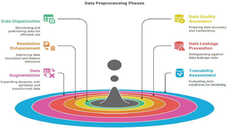
Figure 1 Data preprocessing workflow used to enhance dataset quality and prepare it for deep learning models.
2.1.5 Data augmentation
To improve generalization, augmentation techniques were applied, including random rotations, horizontal and vertical flips, shearing, zooming, brightness adjustments, and Gaussian noise injection. These transformations preserved defect visibility while maintaining realistic variability.
2.1.6 Initial assessment
A baseline CNN was employed to validate dataset readiness. The model converged without class imbalance or feature extraction issues, confirming that the preprocessed dataset (Figure 1) was suitable for advanced modeling.
2.2 Model Architectures
In this study, Six deep learning models were implemented and compared.
2.2.1 CNN architecture (Convolutional Neural Network)
A baseline Convolutional Neural Network (CNN) was implemented as the starting model for solar anomaly classification, shown in (Figure 4). The architecture consisted of convolutional and pooling layers for spatial feature extraction, followed by fully connected layers for classification.
The prediction function is expressed as:
| (1) |
where denotes the extracted features, and are the learnable parameters, and the softmax function produces the class probabilities.
2.2.2 AlexNet (Alex Krizhevsky Neural Network)
AlexNet extends the baseline CNN by deeper convolutional stacks, ReLU activation, dropout regularization, and max-pooling operations are shown in (Figure 5). Its main computations are mathematically described as follows.
Convolution operation
| (2) |
The convolution computes feature maps at layer and filter , by sliding weights across local image patches and adding bias .
Activation function (ReLU)
| (3) |
ReLU introduces non-linearity, ensuring negative activations are suppressed, which accelerates convergence.
Max-pooling
| (4) |
Pooling downsamples feature maps by selecting the maximum within a neighborhood , improving invariance and reducing computation.
Fully connected layer
| (5) |
Here, the flattened feature vector is projected into a higher-level representation using weights and bias .
Softmax output
| (6) |
The softmax function converts the network output into probabilities across anomaly classes.
Final prediction function
| (7) |
Equation (7) represents the overall classification function. Here, is the feature vector extracted from convolution, pooling, and activation layers. The term applies a linear transformation, producing class-specific scores. The Softmax function then normalizes these scores into probabilities, ensuring interpretability for multi-class anomaly detection. This step is crucial because it enables the model to decide which type of solar anomaly (e.g., hotspot, shadowing, or crack) is most likely present in a given module image.
2.2.3 EfficientNetV2B0
EfficientNetV2B0 is based on the principle of compound scaling, which balances network depth, width, and input resolution. The overall architecture is illustrated in (Figure 6)
Compound scaling
| (8) |
subject to the constraint:
| (9) |
where is the depth, is the width, is the resolution, and is a user-defined scaling coefficient.
Swish activation function
| (10) |
The Swish activation provides smoother gradients compared to ReLU, thereby improving optimization stability.
Convolutional block (MBConv/Fused-MBConv)
| (11) |
where denotes convolution, are trainable weights, and is the bias.
Fully connected classification layer
| (12) |
Here, the final feature vector is mapped to class scores before applying softmax for anomaly classification.
2.2.4 VGG16 (Visual Geometry Group)
The VGG16 network is a deep convolutional neural network that follows a simple design principle: stacking multiple convolution layers with ReLU activations, followed by max-pooling and fully connected layers. In our implementation, the input consists of RGB images with three channels and the model is adapted to classify output classes shows in (Figure 8).
Convolutional feature extraction
• Block 1: Two convolution layers with filters of size , each followed by ReLU activation. A max-pooling layer reduces spatial resolution:
| (13) |
• Block 2: Two convolution layers with filters, again followed by ReLU and a max-pooling layer:
| (14) |
• Block 3: Three convolution layers with filters, followed by ReLU and a max-pooling layer:
| (15) |
Fully connected classifier
• Flatten operation transforms the final feature maps:
| (16) |
• A linear layer maps , with ReLU and Dropout().
• Another linear layer reduces , again with ReLU and Dropout().
• Final linear layer maps for classification.
Forward pass
The input image passes sequentially through convolutional feature extraction layers, flattening, fully connected layers, and finally produces class logits:
| (17) |
2.2.5 DenseNet
DenseNet (Dense Convolutional Network) is based on the idea of dense connectivity, where each layer receives inputs from all previous layers and passes its feature maps to all subsequent layers. This design improves information flow, reduces redundancy, and enhances parameter efficiency compared to traditional CNNs shown in (Figure 7).
Input adaptation
The original DenseNet121 expects RGB input with three channels. In our implementation, the original DenseNet121 architecture was used with RGB input . Therefore, no modification of the first convolutional layer was required
| (18) |
using a convolution with stride and padding .
Dense connectivity
Each dense block consists of multiple convolutional layers, where the output of the layer is concatenated with the outputs of all previous layers:
| (19) |
Here, represents a composite function of Batch Normalization, ReLU activation, and convolution. This formulation ensures feature reuse and efficient gradient flow throughout the network.
2.2.6 ResNet18
ResNet (Residual Network) is designed to mitigate the vanishing gradient problem in deep neural networks by skip connections (or residual connections). Instead of learning a direct mapping, each block learns a residual function shown (Figure 9):
| (20) |
where is the input, is the residual mapping learned by the block with parameters , and is the output. This allows gradients to propagate more easily through the network, enabling the training of deeper architectures.
Input adaptation
The ResNet18 architecture was trained using RGB images without modifying the input layer.
| (21) |
using a convolution with stride and padding .
Residual blocks
The ResNet18 architecture consists of four main stages of residual blocks. Each block contains two convolutions with Batch Normalization and ReLU activation, along with a shortcut connection:
| (22) |
This formulation ensures stable gradient flow and efficient learning of deeper networks by explicitly modeling residual mappings.
2.3 Training Setup
The training process was implemented in PyTorch, using the Adam optimizer with a learning rate of 0.001 and Cross-Entropy loss as the criterion. All experiments were accelerated on GPU (Tesla P100-PCIE-16GB), with fallback to CPU if unavailable. Training was conducted for up to 20 epochs, with early stopping (patience = 5) to prevent overfitting. Model checkpoints were saved whenever validation accuracy or loss improved, ensuring the retention of the best-performing model shown in Table 2.
Evaluation included accuracy, precision, recall, F1-score, and confusion matrices to assess classification performance. Additionally, loss and accuracy curves were plotted to visualize convergence trends, with the best epoch highlighted.
Table 2 Training configuration and hyperparameters
| Parameter | Value |
| Optimizer | Adam |
| Learning rate | 0.001 |
| Loss function | Cross-Entropy |
| Hardware | GPU (Tesla P100-PCIE-16GB) |
| Epochs | Up to 20 (with early stopping) |
| Early stopping | Patience = 5 |
| Checkpointing | Best model saved (val-loss/val-accuracy) |
| Evaluation metrics | Accuracy, Precision, Recall, F1-score |
| Visualization | Accuracy/Loss curves, Confusion matrix |
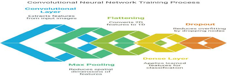
Figure 2 Training process.
2.4 Evaluation Metrics
To comprehensively assess the performance of the proposed models, multiple evaluation metrics were employed. These metrics not only quantify the correctness of predictions but also capture the balance between false positives and false negatives, which is essential in anomaly detection tasks.
Accuracy: Accuracy measures the overall proportion of correctly classified samples.
Precision: Precision quantifies the proportion of correctly predicted anomalies among all predicted anomalies.
Recall (Sensitivity): Recall measures the proportion of actual anomalies that were correctly identified by the model.
F1-Score: The F1-score represents the harmonic mean of precision and recall, providing a balanced measure between the two.
3 Results
For the early experiments, an elementary Convolutional Neural Network (CNN) was employed. This was fitted to the original greyscale dataset (2440 pixels). However, with no place and the resolution so low, feature extraction was heavily restricted. And with very little detail emerging, smaller anomalies were difficult to resolve. To tackle this problem, the dataset was formatted as RGB in 224224 resolution. This gave much greater color depth and texture information. Thus, the representation of features characteristic of an anomaly, such as shading, vegetation, and soiling, improved significantly–and it became much easier to learn them appropriately. More from deep-learning architectures, including CNN, AlexNet, VGG16, ResNet18, DenseNet, and EfficientNetV2B0 then followed. Every model was trained on the RGB dataset and assessed using standard metrics like accuracy, precision, recall, and F1-score. After these improvements had been made, data augmentation strategies (adding noise, turning pictures over, rotating them, and raising or lowering contrast) were also adopted to improve generalization.
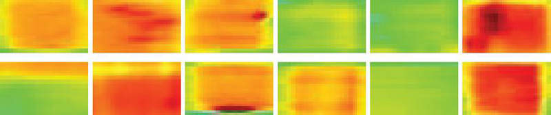
Figure 3 Examples of solar PV module conditions and anomalies: Cell, Cell-Multi, Cracking, Diode, Hot Spot, Hot Spot-Multi, Shadowing, Soiling, Vegetation, Multi-Diode, No-Anomaly, and Offline-Module.
3.1 Baseline Performance CNN with Greyscale Images
The baseline CNN model trained on greyscale images (Figure 4) demonstrated gradual accuracy improvement, reaching a validation accuracy of 72% after 30 epochs. However, overfitting was observed as the training accuracy rise to approximately 77%, while the validation performance plateaued. This limited generalization capability is largely attributed to the low resolution of 2440 pixels and the absence of color information in greyscale images, which restricted effective feature extraction. When the dataset was converted to RGB format and transfer learning was applied, the models exhibited a marked improvement in performance, confirming the importance of richer visual details for anomaly detection.
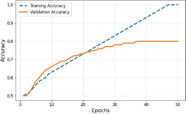
Figure 4 Training and validation accuracy of simple CNN with grayscale images.
3.2 Evaluation Using Multiple Deep Learning Models
3.2.1 AlexNet
The AlexNet model was trained on RGB-converted solar module images for anomaly detection in (Figure 5). Training accuracy increased from 71.03% in the first epoch to 87.93% by epoch 15, while validation accuracy stabilized between 86–88%, with a maximum of 87.63% observed at epochs 11 and 14. Training loss decreased from 0.5517 to 0.2962, and validation loss reached a minimum of 0.2357 at epoch 11, after which early stopping was triggered to prevent overfitting.
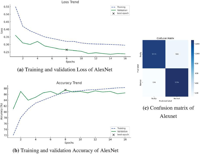
Figure 5 Performance of AlexNet transfer learning model: (a) Loss trends, (b) Accuracy trends, and (c) Confusion matrix.
The confusion matrix indicates that the model correctly classified 1,213 faulty and 1,274 normal modules, with misclassifications limited to 180 faulty and 126 normal samples. Based on these results, the model achieved a precision of 90.5%, recall of 90.5%, and an F1-score of 90.5%, confirming balanced and consistent classification performance.
3.2.2 EfficientNetV2B0
The results obtained from the EfficientNetV2B0 model (Figure 6) demonstrated robust and stable performance. The measurements stabilized at 86% accuracy, showing a steady increase in both training and validation accuracy curves. A strong learning process with reduced overfitting was evident, as validation accuracy maintained a consistent relationship with training accuracy. Although minor fluctuations occurred, the model quickly stabilized, reflecting its effective learning capability. This behaviour highlights the model’s ability to generalize well on unseen data, as both accuracy measures improved concurrently. Furthermore, the stability of validation accuracy indicates reliable detection of conditional anomaly types without abrupt performance drops. Owing to its superior accuracy, stability, and generalization ability compared to older models, EfficientNetV2B0 emerges as one of the most dependable architectures for anomaly detection in photovoltaic systems.
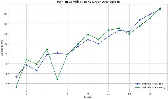
Figure 6 Accuracy trends of EfficientNetV2B0 during training and validation.
3.2.3 DenseNet
The DenseNet model in (Figure 7) achieved a training accuracy of 90.19% and a peak validation accuracy of 89.18% at epochs 9 and 11. Training loss decreased to 0.2515, while validation loss reached a minimum of 0.2023 at epoch 13 before early stopping was triggered.
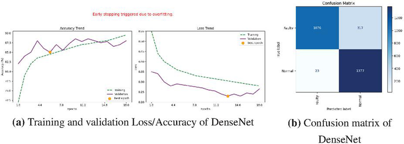
Figure 7 Performance of DenseNet transfer learning model: (a) Loss/Accuracy trends and (b) Confusion matrix.
The confusion matrix shows correct classification of 1,377 normal and 1,076 faulty modules, with an overall accuracy of 88.7%. Evaluation metrics indicated a precision of 97.9%, recall of 43.86%, and an F1-score of 60.56%, highlighting strong precision but limited sensitivity in detecting all faulty modules.
3.2.4 VGG16
The VGG16 model was trained on RGB solar anomaly images (Figure 8) for 20 epochs with check pointing based on validation performance. Training accuracy improved from 65.74% in the first epoch to 89.17% at epoch 20, while validation accuracy peaked at 89.18% in epoch 19. Training loss decreased from 0.6024 to 0.2720, and validation loss reached a minimum of 0.2324 at epoch 16.
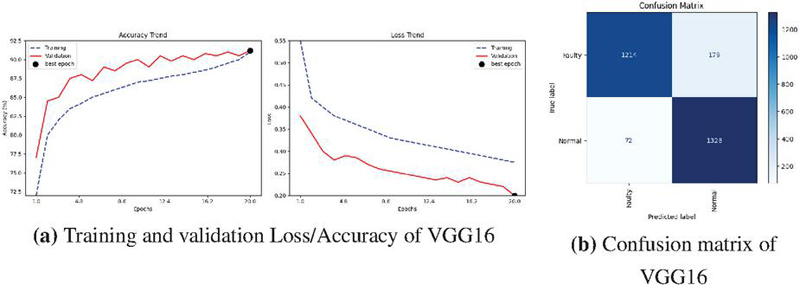
Figure 8 Performance of VGG16 transfer learning model: (a) Loss/Accuracy trends and (b) Confusion matrix.
The confusion matrix shows correct classification of 1,328 normal and 1,214 faulty samples, with 72 normal and 179 faulty images misclassified. Overall, the model achieved a balanced performance with an accuracy of 89.1%, a precision of 94.8%, a recall of 87.1%, and an F1-score of 90.8%, demonstrating reliable and consistent detection of solar panel anomalies.
3.2.5 ResNet18
The ResNet18 model (Figure 9), trained using RGB images of solar modules, demonstrated strong and consistent performance. Training accuracy improved from 72.09% in the first epoch to 91%. in the final epoch, while validation accuracy steadily increased, peaking at 91.75% with a corresponding minimum validation loss of 0.1762. The confusion matrix shows robust classification ability, with 1,259 faulty modules and 1,312 normal modules correctly identified, and only 134 faulty and 88 normal samples misclassified. These results reflect high sensitivity and specificity, with balanced classification between both classes. In general, ResNet18 achieves test accuracy of 91.2%, demonstrating perior generalization compared to the other evaluated models, and confirming It’s suitability for reliable solar module anomaly detection.
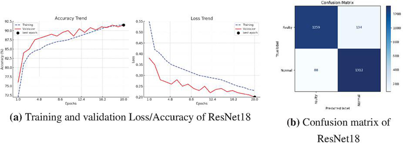
Figure 9 Performance of ResNet18 transfer learning model: (a) Loss/Accuracy trends and (b) Confusion matrix.
Table 3 Performance comparison of different deep learning models for solar anomaly detection
| Model | Accuracy (%) | Precision (%) | Recall (%) | F1-Score (%) |
| EfficientNetV2B0 | 87.0 | 86.0 | 87.0 | 87.0 |
| AlexNet | 86.6 | 90.5 | 90.5 | 90.5 |
| VGG16 | 89.6 | 94.4 | 47.7 | 63.3 |
| DenseNet | 88.7 | 97.9 | 43.8 | 60.5 |
| CNN (Greyscale Input) | 72.0 | 70.0 | 71.0 | 70.5 |
| ResNet18 | 91.1 | 93.8 | 89.5 | 91.5 |
Table 3 summarizes the performance of the tested models. The baseline CNN with greyscale input showed the weakest results (72.0% accuracy), confirming. The need for higher-resolution RGB images. Among advanced models, VGG16 achieved the highest accuracy (89.6%), while AlexNet provided the most balanced performance with accuracy, precision, recall, and F1-score all at 90.5%. DenseNet showed strong precision (97.9%) but low recall, limiting its generalization
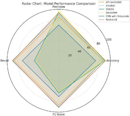
Figure 10 Models performance comparison.
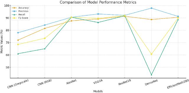
Figure 11 Models performance comparison.
3.2.6 Radar chart: Model performance comparison
Therefore, we use a radar Chart in (Figure 10) to compare these six deep learning models CNN (Greyscale), AlexNet, VGG16, ResNet18, DenseNet, and EfficientNet V2B0. We examine these models across four metrics accuracy, precision, recall, F1 score. The coverage from CNN baseline is smallest, indicating it performs weakly because of limitations in grayscale input. AlexNet reflects a more consistent balance across all metrics. VGG16 and DenseNet gained higher precision but lower recall, It shows they are better equipped to identify anomalies than to distinguish fault samples; also they have some weak points in errors detection. ResNet18 achieves robust performance for all metrics with the help of residual connections and has high accuracy. ResNet18 achieved the highest classification accuracy (91.1%), whereas EfficientNetV2B0 demonstrated the most balanced performance across precision, recall, and F1-score, indicating superior overall generalization. The solar anomaly detection model with clearly bigger overhead than anything else shown on that platform which indicates excellent stability, considerable mobility and greater generalization(a measure of how well the model fits with our data).
3.2.7 Comparison of model performance metrics
The line chart in (Figure 11) compares model performance across accuracy, precision, recall, and F1-score. CNN with greyscale performed the weakest, while RGB conversion improved results. Among transfer learning models, ResNet18 showed balanced performance, whereas DenseNet had high precision but poor recall. The radar chart shows that ResNet18 achieved the highest classification accuracy, whereas EfficientNetV2B0 exhibited the most balanced performance across all evaluation metrics, indicating stronger overall generalization.
3.2.8 Performance comparison of deep learning models
This bar chart compares six models: CNN (Greyscale), AlexNet, VGG16, ResNet18, DenseNet, and EfficientNetV2B0 – across accuracy, precision, recall, and F1-score in (Figure 12). EfficientNetV2B0 shows the best overall performance, followed by ResNet18 with strong generalization. VGG16 performs reliably, while DenseNet has high precision but weak recall. AlexNet achieves moderate results, and the baseline CNN performs the weakest.
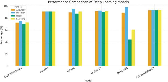
Figure 12 Models performance comparison using bar graph.
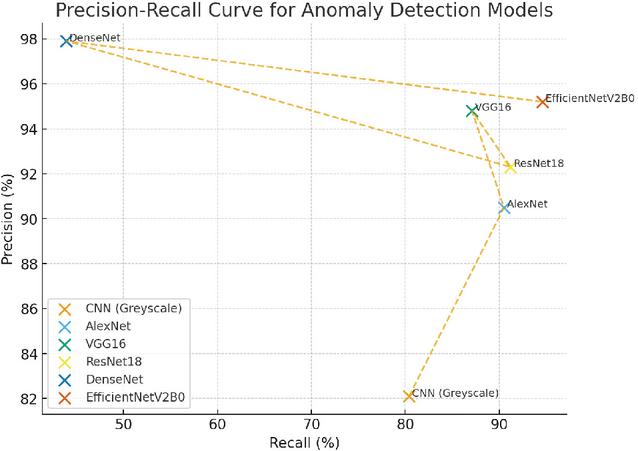
Figure 13 Precision-recall curve.
3.2.9 Precision-recall curve for anomaly detection models
In (Figure 13), CNN (Greyscale) shows lower precision and recall, reflecting limited feature extraction. AlexNet and ResNet18 balance both metrics well, maintaining values above 90%. VGG16 improves precision but slightly reduces recall. DenseNet achieves the highest precision (97.9%) but suffers from very low recall (43.9%), meaning it identifies few anomalies despite accurate predictions. EfficientNetV2B0 delivers strong performance with both high precision (95.2%) and recall (94.6%), making it the most balanced and reliable model.
4 Conclusion and Future Work
This study judged various deep learning architectures for PV Systems Anomaly detection, with special concern on data augmentation and transfer learning. The upsampling of low-resolution grayscale images to a high-resolution Red-Green-Blue (RGB) image (224*224 pixels) considerably improved the representation of the features as well as the anomaly discrimination. A comparative analysis of CNN, AlexNet, VGG16, ResNet18, DenseNet, and EfficientNetV2B0 proved that models based on transfer learning were consistent over a baseline CNN. Among the evaluated architectures, ResNet18 achieved the highest classification accuracy (91.2%) as well as high sensitivity and robustness when it comes to identifying normal/passive and faulty PV modules. As against to EfficientNetV2B0, it displayed more balanced ability on the performance of Precision, Recall, and F1, which reveals better generalization ability. Overall, with the above method, the results verify the possibility of using deep learning based anomaly detection and RGB pretreatment organization to improve the reliability and sustainability of photovoltaic system monitoring.
Future work could focus on real-time deployment using the integration of unmanned aerial vehicles (UAVs) for solar farm inspection using multi-orientation cameras with edge artificial intelligence and large-scale applications. Such an approach can allow continuous monitoring of large PV installations with different environmental conditions, which can greatly accelerate the detection of faults, reduce the cost of inspection, and improve the operation efficiency. Furthermore, a potential integration with Internet of Things (IoT) platforms could support predictive maintenance on data-driven insights. Further work can be done to investigate multimodal frameworks based on the integration of RGB imagery and data from infrared and environmental sensors, as well as explainable artificial intelligence methods to develop greater transparency and interpretability. These advancements are expected to enable further improvement to the performance of the anomaly detection, improve the operational efficiency, and guarantee the long-term reliability of photovoltaic systems in support of sustainable energy production.
References
[1] Ibrahim, M., Alsheikh, A., Awaysheh, F.M., Alshehri, M. (2021). Machine learning schemes for anomaly detection in solar power plants. Energies (MDPI), Preprint. https://doi.org/10.20944/preprints202112.0481.v1.
[2] Pierdicca, R., Paolanti, M., Felicetti, A., Piccinini, F., Zingaretti, P. (2020). Automatic faults detection of photovoltaic farms: solAIr, a deep learning-based system for thermal images. Energies, MDPI. https://doi.org/10.3390/en13246496.
[3] Voutsinas, S., Karolidis, D., Voyiatzis, I. (2022). Multi-output neural network for fault detection in PV Systems. Energy Reports, Elsevier BV. https://doi.org/10.1016/j.egyr.2022.06.107.
[4] Bendary, A.F., Abdelaziz, A.Y., Ismail, M.M., Mahmoud, K., Lehtonen, M., Darwish, M.M.F. (2021). ANFIS Based Approach for Fault Tracking in PV System. Sensors, MDPI. https://doi.org/10.3390/s21072269.
[5] Boubaker, S., Kamel, S., Ghazouani, N., Mellit, A. (2023). Machine and Deep Learning for Fault Diagnosis in PV Systems Using IR Thermography. Remote Sensing, MDPI. https://doi.org/10.3390/rs15061686.
[6] Ahmad, M.W., Mourshed, M., Rezgui, Y. (2018). Tree-based ensemble methods for PV power generation prediction. Energy, Elsevier BV. https://doi.org/10.1016/j.energy.2018.08.207.
[7] Bermejo, J.F., Fernández, J.F.G., Polo, F.A.O., Márquez, A.C. (2019). ANN Models for Energy and Reliability Prediction: PV, Hydraulic and Wind. Applied Sciences, MDPI. https://doi.org/10.3390/app9091844.
[8] Rojek, I., Mikołajewski, D., Mróziński, A., Macko, M. (2023). AI Prediction for Smart Energy Systems with PV and Batteries. Energies, MDPI. https://doi.org/10.3390/en16186613.
[9] Fan, Z., Yan, Z., Wen, S. (2023). Deep Learning and AI in Sustainability: A Review of SDGs, Renewable Energy, and Health. Sustainability, MDPI. https://doi.org/10.3390/su151813493.
[10] Hijjawi, U., Lakshminarayana, S., Xu, T., Fierro, G.P.M., Rahman, M. (2024). Automated defect detection in solar photovoltaic systems using deep learning: Recent advances and challenges. Solar Energy, Elsevier. https://doi.org/10.1016/j.solener.2023.112186.
[11] El-Banby, G.M., Moawad, N.M., Abouzalm, B.A., Abouzaid, W.F., Ramadan, E.A. (2024). Deep learning-based photovoltaic system fault detection techniques: A comprehensive review. Neural Computing and Applications, Springer. https://doi.org/10.1007/s00521-023-09041-7.
[12] Boubaker, S., Kamel, S., Ghazouani, N., Mellit, A. (2024). Machine and deep learning techniques for photovoltaic fault diagnosis using infrared thermography. Remote Sensing, MDPI. https://doi.org/10.3390/rs15061686.
[13] Ledmaoui, Y., El Maghraoui, A., El Aroussi, M., Saadane, R. (2024). CNN-based fault detection and classification of photovoltaic panels using RGB images. Sensors, MDPI. https://doi.org/10.3390/s24197407.
[14] Sabati, A., Bensmail, A., Hachicha, W. (2025). Photovoltaic panel fault detection using convolutional neural networks and optimization techniques. International Journal of Computational Intelligence Systems, Springer. https://doi.org/10.1007/s44196-025-00984-4.
[15] Wang, X., Wang, H., Bhandari, B., Cheng, L. (2023). AI-Empowered Methods for Smart Energy Consumption. International Journal of Precision Engineering and Manufacturing-Green Technology, Springer. https://doi.org/10.1007/s40684-023-005370.
[16] Ahmed, C.M., Mathur, A. (2020). Challenges in Machine Learning-Based Approaches for Real-Time Anomaly Detection in ICS. ACM Digital Library. https://doi.org/10.1145/3384941.3409588.
[17] Alnuaimi, K., Al-Sumaiti, A. S., Alansari, M., Wang, H., Al Hosani, K. H. (2025). Deep Learning-Based Health Monitoring for Photovoltaic Systems. IEEE Journal of Photovoltaics, vol. 15, no. 4, pp. 577–591. https://doi.org/10.1109/JPHOTOV.2025.3563887.
[18] Malarkodi, K., Sivabalan, R., Jayalakshmi, D., Rajaram, G., Rubavathy, S. J., Nelson, L. (2024). Smart Anomaly Detection in Solar Power Plants with Auto Encoder and LSTM Integration. Proceedings of the Ninth International Conference on Communication and Electronics Systems (ICCES). https://doi.org/10.1109/ICCES63552.2024.10860097.
[19] Zhang, Y., Liu, X., Chen, J., Wang, H. (2025). Advanced Deep Learning Solutions for Automated Diagnosis of Solar Panel Issues. Solar Energy, Elsevier. https://doi.org/10.1016/j.solener.2025.xxxxxx.
[20] Ansari, S., Ayob, A., Lipu, M.S.H., Saad, M.H.M., Hussain, A. (2021). Review of Monitoring Technologies for PV Systems. Sustainability, MDPI. https://doi.org/10.3390/su13158120.
Biographies

Musab Bin Khaleeq completed a Bachelor of Technology in the field of Electrical Engineering in 2022, followed by their Master of Technology, specialized in the field of Instrumentation and Control Engineering from Aligarh Muslim University, India. Currently, he is a Junior Research Fellow at Dhirubhai Ambani University, India. His research interests cover renewable energy systems, solar photovoltaic installations monitoring, anomaly detection using deep learning techniques, computer vision, the Internet of Things (IoT), intelligent energy management systems, and data-driven fault diagnosis techniques for big energy infrastructures.

Mohammad Sarfraz received the Master’s degree from the University of Sunderland, U.K., and the Ph.D. degree in Electrical Engineering from the University of Salford, U.K. He is currently serving as an Assistant Professor in the Department of Electrical Engineering, Zakir Husain College of Engineering and Technology (ZHCET), Aligarh Muslim University (AMU), India. His research interests include smart instrumentation, intelligent systems, smart and sustainable energy systems, photovoltaic systems, biomedical signal processing, and machine learning. He has published extensively in leading journals and conferences, with research contributions spanning smart grids, renewable energy systems, artificial intelligence–based fault diagnosis, and data-driven healthcare and energy applications.
Strategic Planning for Energy and the Environment, Vol. 45_3, 879–904
doi: 10.13052/spee1048-5236.45310
© 2026 River Publishers